Interactive Feature Space Explorer© for Multi–Modal Magnetic Resonance Imaging

Abstract

Wider information content of multi–modal biomedical imaging is advantageous for detection, diagnosis and prognosis of various pathologies. However, the necessity to evaluate a large number images might hinder these advantages and reduce the efficiency. Herein, a new computer aided approach based on the utilization of feature space (FS) with reduced reliance on multiple image evaluations is proposed for research and routine clinical use.

The method introduces the physician experience into the discovery process of FS biomarkers for addressing biological complexity, e.g., disease heterogeneity. This, in turn, elucidates relevant biophysical information which would not be available when automated algorithms are utilized. Accordingly, the prototype platform was designed and built for interactively investigating the features and their corresponding anatomic loci in order to identify pathologic FS regions.

While the platform might be potentially beneficial in decision support generally and specifically for evaluating outlier cases, it is also potentially suitable for accurate ground truth determination in FS for algorithm development. Initial assessments conducted on two different pathologies from two different institutions provided valuable biophysical perspective. Investigations of the prostate magnetic resonance imaging data resulted in locating a potential aggressiveness biomarker in prostate cancer. Preliminary findings on renal cell carcinoma imaging data demonstrated potential for characterization of disease subtypes in the FS.

1 Introduction

By inferring various biophysical, chemical and structural tissue properties, biomedical imaging enables the detection of tissue states (e.g., benign or malignant) for diagnostic and/or prognostic purposes. For example, tissue water content assessment with T₂–weighted (T2W) magnetic resonance imaging (MRI) and inference of microstructure by diffusion weighted (DW) MRI are standard techniques utilized in different organs for various diseases, disorders, (e.g., a variety of neurological conditions [1]) and damage types (e.g., diffuse and local brain injuries [2]). Furthermore, new methods are being developed to explore new biophysical avenues, e.g., tissue magnetic properties [3].

However, there are pathologies where considerable signal overlaps exist between malignant and benign conditions in individual modalities. This in turn hinders or prevents successful categorization. By contrast, inclusion of multiple imaging modalities increases information content, thereby providing better assessment accuracy. For instance, in the prostate, where benign prostatic hyperplasia (BPH) and prostate cancer (PCa) might be indistinguishable with T2W–MRI alone [4], the addition of apparent diffusion coefficient (ADC) maps improves the detection and characterization of cancer foci [5], [6], [7].

A significant challenge imposed by a wider usage of the multi–modality imaging is the necessity to longitudinally evaluate a large number of images obtained from multiple anatomic sections with different imaging modalities (e.g., MRI, positron emission tomography (PET)) and sub–modalities (e.g., ADC, T2W in the case of MRI). This massive amount of data impedes the efficiency of initial and longitudinal evaluations in management strategies, such as active surveillance in PCa [8] as it requires a considerable effort that is highly susceptible to inter–and intra–observer variability [9], [10], [6], [11]. This subjectivity might result in misdiagnosis and potentially in mistreatment of the patient, and therefore might have serious consequences. Moreover, as new imaging methods are added to the multi–modal information pool, there might be a time lag before sufficient clinical expertise is widely available, especially in highly complex diseases such as PCa [12]. Accordingly, there might be advantages to presenting the essence of multi–modal imaging data in a compact manner for usage in research, development and the clinic.

Herein, a computer aided visualization and decision technique, which assembles several tissue properties in a single entity, is introduced with a prototype implementation. Its essence is the exploration of the entirety of these properties originating from all of the images instead of multiple individual image evaluations. The foundation of the technique comprises the feature space (FS), which is constructed by combining signals from different imaging modalities into points in high–dimensional spaces as described in Section 2. Therein, the whole is greater than its parts because regardless of their anatomic location, all of the tissues with similar multi–modal imaging properties are projected onto the same neighborhoods within the FS. Reciprocally, the features contained in a given FS neighborhood are shared by multiple anatomic regions. By using this principle, the method herein assists in locating malignant and benign FS regions in order to identify the complete anatomical disease burden in a single instance.

Under ideal conditions, if known, an appropriate combination of biomedical imaging signals specifically sensitive to discriminating biophysical properties of the investigated pathology would be utilized. This would create in the FS homogenous, i.e., unmixed malignant and benign features, even more desirably, separated neighborhoods thereof.

In general, however, biological complexity with its possibly infinite dimensionality prevents such a clear–cut scene. Signal overlaps occur as each imaging modality projects the infinite dimensional biophysical FS onto its lower dimensional detection range, e.g., T2W prostate MRI described above. Ultimately, the homogeneity of the FS neighborhoods is determined by the level of specificity and sensitivity that imaging modalities can provide. The extent of insufficiencies depends on the disease and its complexity. A challenging example discussed in Section 4 is PCa, which possess ‘mimics’ even in multi–modal imaging [13].

For each organ and various pathologies the task is therefore twofold: determining the necessary and sufficient imaging modalities, and identifying the significant FS regions. The latter is a building block for addressing the former, which is a future research topic that will be addressed by assessing various modality combinations

Without a common avenue for locating malignant FS regions applicable to various pathologies, manual FS investigations are highly valuable for understanding and interpreting multi–modal imaging data. For instance, in Section 5, the individual FS analysis verified recent findings about different subtypes of renal cancer. Likewise, in a clinical environment where complex disease and/or unusual cases are encountered, relevant decision assistance might potentially be obtained. Furthermore, the lack of separation between FS neighborhoods is perhaps the biggest challenge of pattern recognition algorithms, such as support vector machines [14], [15] and discriminant analysis [16]. Accordingly, important insight might be obtained with exploration of the multi–modal data by medical experts in a research or clinical environment. For example, during automated method development, determining ground truth by direct exploration of the FS, where the algorithms operate, might be potentially more accurate than currently used manual identification on multi–modal images.

Here, the prototype of an interactive evaluation environment for manually locating suspicious and malignant features is implemented. The software package described in Section 3 equips the user with the capability to visualize the bi–directional correspondence between features and anatomic loci. Named after its interactive implementation of this exploration capability, Interactive Feature Space Explorer^© (InFS–Explorer^© or InFSExp^© or InFSE^©) relies on the user’s expertise to identify regions of interest (ROI) within the FS. The interactive process involves an adjustment procedure by shuttling between the FS and anatomic regions until the satisfaction of the specialist. In a sense, InFS–Explorer^©’s graphical user interface (GUI) translates the specialist’s knowledge into practice during the discovery of FS ROIs.

2 An Overview of the Feature Space

The FS framework, which had been previously used in satellite image processing systems, was applied to MR images [17] about three decades ago. Later, FS was further utilized in segmentation and classification problems for various anatomies [18]. In this section, an overview of the FS is presented.

In biomedical images, the signal intensity at each pixel is defined by the measurement obtained from the pixel’s anatomical location. As each signal depends on specific tissue properties, maps and images of the same anatomy reflect different intensity and contrast levels as shown in the ADC map and T2W images of Fig. 1.

Figure 1.

The construction of a 2–dimensional feature space defined by the ADC map and the scaled T2W intensities from a 62 year old patient with PCa. All of the feature vectors originating from the whole gland are visualized as a scatter plot. A 2 dimensional histogram of the feature vectors, on the right, is overlaid on the scatter of points to color code the number of pixels indicated by the bar on the right. The light blue color towards the bulge indicates a relatively large volume associated with bulge features.

In this manuscript, the feature vector at a given anatomic location is constructed by stacking the signal values from each modality into an array of numbers. The entries of the feature vector can originate from various biomedical imaging modalities such as computed tomography (CT), PET and MRI, as well as maps and sub–modalities (e.g., Fluorodeoxyglucose (FDG) PET, T₁–weighted (T1W) and T2W images, diffusion, T₁ and T₂ maps of MRI, etc.). Mathematically, the feature vectors live in a space of dimension equal to the number of imaging modalities used in data acquisition, i.e., FS⊂ℝ^m where m denotes the number of modalities. More formally

$$FS=\{{[f_1(x)\dots f_m(x)]}^T\mid x\in V\subset {ℝ}^3\}$$

where f_i is the signal from the i^th modality, x denotes the voxel location and V is the anatomic volume of interest. For example, in Fig. 1, FS = {[ADC(x)T₂(x)]^T| x∈Prostate}.

The content of the FS is visualized by plotting vectors gathered from all of the pixels in the multi–slice volume (see Fig. 1). Each feature vector is shared by multiple pixels exhibiting the same properties. Accordingly, if the location of features of interest (e.g., malignant) is known, disease burden is presented anatomically (see Section 3) by visualizing anatomic regions with those features. This one–to–many association from the FS to the anatomic locations makes determining the malignant FS regions the epicenter of the approach. Consequently, the biomarker value of the FS is based on locating the neighborhoods containing pathologic tissue features. Once known, these malignant features can identify anatomic loci that might otherwise be missed when images are analyzed individually.

In practice, when constructing the FS from multi–modal imaging data, possible inter–modal image resolution mismatches need to be eliminated using co–registration techniques (see Section 3). In addition, modality specific artifacts, such as image distortions, should be corrected before creating the feature vectors. More generally, global systematic changes such as a constant signal shift, i.e., f_i(x)+c_i, will not necessarily affect FS evaluations as they displace the entirety of feature points in the i^th dimension without affecting the relative location of malignant and benign FS sets. However, local artifacts dependent on voxel positions, i.e., f_i(x)+Δf_i(x) f_i(x)+, might mischaracterize biophysical tissue properties at those locations and therefore need careful treatment. For example, the intensity inhomogeneity in MR images is adjusted [19] prior to evaluation. On the other hand, smaller perturbations where Δf_i(x) remains at the noise level do not necessarily require adjustments as they will not displace largely the points inside the FS neighborhoods. As the aforementioned issues manifest differently for various modalities and anatomies without a common solution, specific preprocessing is generally required for individual combinations.

Earlier works adopted the FS for the purpose of tissue classification by identifying ellipsoid neighborhoods in the FS [17], segmentation using various methods including feature extraction [18] and optimizing mathematical transformations of the FS for clustering normal tissue’s feature points at predefined target positions [20] for a standardized analysis.

However, in challenging pathologies the complexity and heterogeneity of the biological tissue necessitate more sophisticated geometric descriptions of FS neighborhoods. PCa is an example, where “it is difficult, if not impossible, to extract specific ranges for individual parameters” [21]. In other words, in PCa simple rectangular ROIs parallel to the coordinate axes of the multi–modal FS cannot capture completely the malignancies. In fact, the malignant FS regions in Figs. 6 and 8 are non–convex and therefore they cannot be obtained by thresholding methods including ellipsoids, linear discriminants and histogram based procedures.

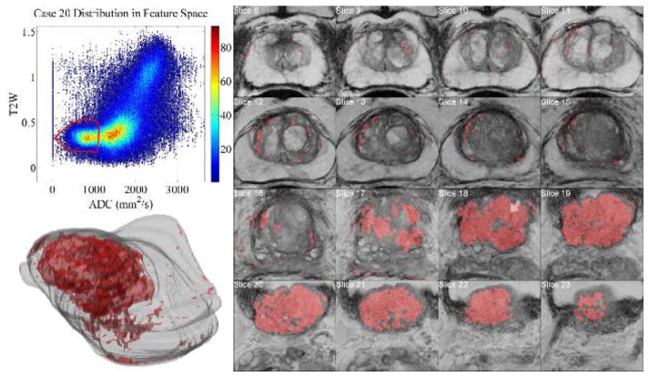
Figure 6.

When the FS ROI is demarcated with the red polygon in MR–FS (81 year old patient outside the cohort described in the text) following the steps in Fig. 4, it highlights multiple pixels suspicious for cancer, demonstrating the one–to–many nature of the correspondence between the FS and the pixels. The correspondence’s confinement to solely suspicious pixels seen on the images and in the whole gland of the 3 D reconstruction from MRI slices demonstrates the potential aggressiveness biomarker value of the FS region.

Figure 8.

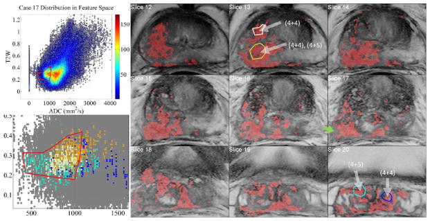
Aggressive case of a 68 yrs. old patient’s positive biopsy loci indicated with white arrows. The inter– and intra–tumor heterogeneity is visualized when biopsy regions are selected with InFS–Explorer^©. Whereas right seminal vesicles’ (SV) (4+5) tumor features (cyan) are distributed towards the tip of the FS bulge, (4+5) right mid–base peripheral zone region (brown) clustered towards the center of the FS and the central gland (4+4) component (white) is dispersed between the cyan and brown features. The dark blue features from (4+4) left SV loci are placed away from the tip of the FS bulge, intermingled with the other feature points. Inclusion (not shown) of the non–convex FS ROI’s north–west corner implicated a benign region on Slice 17 (green arrow).

One of the important goals of FS analysis is the description of the FS regions encapsulating all of the suspicious features regardless of the number of anatomic pixels sharing those. In PCa, this is equivalent to the detection and staging of “small albeit significant tumors” [22]. Missing one aggressive pixel during individual image evaluation, might potentially be avoided by using the FS.

The strategy is then the direct investigation of properties on the FS rather than replicating simultaneous evaluation of anatomical images from different modalities by a human observer as is most commonly attempted. Described mathematically, the total multi–modal (FS and imaging) space is modeled as Σ = ℝ^m × ℝ³, where ℝ^m is the FS obtained from m different modalities and ℝ³ is the anatomic location space. InFS–Explorer^© works according to the following commutative diagram:

$$\begin{array}{ccc}{ℝ}^m& \times & {ℝ}^3\\ \downarrow & & \downarrow \\ {ℝ}^m& \rightleftarrows & {ℝ}^3\end{array}$$ (1)

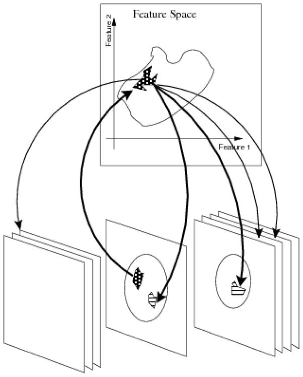
The basic operation implemented by InFS–Explorer^© ’s GUI relies on the correspondence of the subsets of FS (ℝ^m) with the anatomic locations (ℝ³) and vice versa as shown in Fig. 2.

Figure 2.

Practical use of the commutative diagram ((1)) as the working principle of InFS–Explorer^©. A suspicious anatomic location, e.g., a lesion observed on a single slice, presents a set of features (upward arrow). In turn, these features are shared by multiple anatomic locations (downward arrows), demonstrating the disease burden based on the FS location.

In addition, the anatomic volume information can be visualized by color coding the histogram of the pixels and overlaying it on the FS scatter plot on the right of Fig. 1 (see also Fig. 3 corresponding to color overlay of Fig. 1, and see Figs. 6, 7 and 8 below for a comparison of tumor burden).

Figure 3.

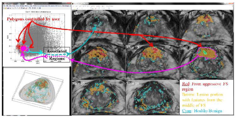
The InFS–Explorer^© GUI workspace for a 62 year old patient with PCa. On both MR–FS (top left) and anatomic images (right), ROIs are drawn interactively showing associated pixels and feature points respectively. Initially, by demarcating the features of the red ROI on Slice 13, the anatomic burden is visualized in red in the anatomic volume. The features of the smaller adjacent green ROI on Slice 14 were covered when the purple ROI was placed on the larger lesion. In turn, when brown and cyan FS ROIs were drawn respectively around the purple and green feature points, PCa’s heterogeneous appearance can be visualized on the anatomical images as well as on the 3 D representation of the gland (bottom, left).

Figure 7.

Tumor burden on a 68 year old patient captured with the demarcation of the bulge in the MR–FS. Prior to the observation of MR images, the large burden can be inferred from the color overlay, which can be also visualized in the 3 D virtual gland. Biopsy (white arrow in MRI) reported a score of (4+4), qualifying the case as aggressive.

3 InFS–Explorer ^©

Pathologies of complex and heterogenous nature might manifest inter– or intra–patient variations, which consequently require individual analysis of the biomedical imaging data. For this purpose, InFS–Explorer^© is designed specifically for physicians to search and validate the FS regions, whereby their cumulative experience and knowledge is translated into identifying relevant tissue properties. The methodology outlined in Section 2 establishes a framework for connecting biological information and data analysis. InFS–Explorer^©’s GUI in Fig. 3 implements the interactive exploration of the FS and anatomic space.

Prior to the GUI’s launch, there are several data preparation steps that must to be completed. First, signals from areas other than the investigated organ might bring additional unnecessary features, enlarging the FS point cloud. As this will conceal the critical features, it might be necessary to generate an appropriate initial mask of the organ volume. InFS–Explorer^© incorporates a rudimentary image intensity thresholding algorithm that would create masks for whole signal volumes (e.g., head volume extraction from a large field of view (FOV)). The program uses half of the mean value of the signal from all of the volume as the threshold for creating binary masks at each slice. Subsequently, the holes in the binary masks are filled by using the imfill function of the Matlab® Image Processing Toolbox®. This simple strategy for creating organ masks has been useful in several cases but specific image processing algorithms (e.g., skull stripping) are beyond the scope of the software. For complicated anatomies, such as the prostate, it is more efficient to externally provide a mask. The mask might be manually prepared –a highly reproducible task in a clinical environment– or automatically generated if successful algorithms exist. InFS–Explorer^© applies the mask over the image volume for obtaining only the features from the anatomy of interest.

Second, depending on the anatomy and the modalities, the images might need to be preprocessed, e.g., patient motion and systematic distortion corrections. Each biomedical imaging modality suffers from its own artifacts and therefore requires its own correction algorithms. It was, therefore, more suitable to keep the preprocessing out of the scope of InFS–Explorer^©.

More importantly, possible image resolution differences between modalities might result in differences of pixel center locations in the anatomic space, ℝ³. Without image co–registration, this location mismatch invalidates the operating diagram ((1)), as stacking features from different positions would be meaningless. In the absence of cross–modality and anatomy specific external co–registration algorithms for resolving the mismatch, InFS–Explorer^© has an option to use the nearest neighbor algorithm on the volume for preserving information content and fidelity. The algorithm was implemented with the standard Matlab® command griddedInterpolant [23] in ℝ³ which subdivides lower resolution voxels (i.e., large) into smaller ones to match the higher resolution voxel locations while keeping the original signal value.

Finally, although calculated maps (e.g., calculated T₂ maps versus T2W intensity images) are quantifiable and may improve the outcomes (e.g., in PCa [24]), acquisition/computation speed makes the utilization of intensity images a necessity in most clinical applications. In multiple patient studies (e.g., aiming for biomarker discovery) and/or longitudinal patient surveillance where quantification is essential, intensity scaling or normalization using the value obtained from a common region is necessary. For example, ROIs from the bladder are utilized for scaling in Section 4 and for normalization in [25].

At the launch of an InFS–Explorer^© instance, the aforementioned steps are achieved with the setup window (not shown) by using drop down menus, forms and check boxes. By default, the setup window names the study after its directory name and the modality data after their file names. All of these settings, which can be modified by the user, are used in labeling various graphs within the GUI. The setup menu gives the option of saving the settings using the study name with a time stamp as the default file name for facilitating the subsequent returns at later times.

Upon completion of the initial preparations, InFS–Explorer^© loads the data and presents the FS and the anatomical images as in Fig. 3. The user has the option to display the FS as a scatter plot, as a contour plot and as overlaid combinations thereof. Similarly, switching between different modality images is possible in the anatomical image window on the right of Fig. 3.

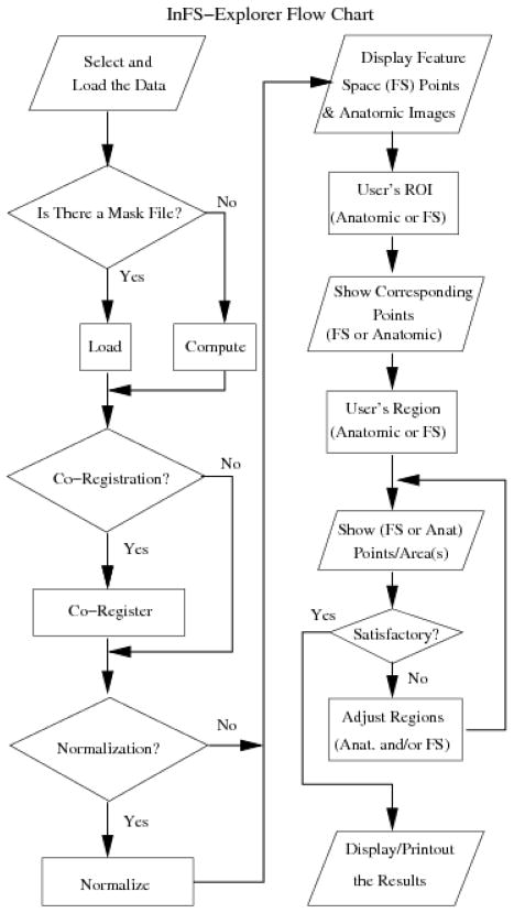
Once FS and anatomic images are visualized, investigations start with demarcating ROIs. Whenever an ROI is created on the FS or on the anatomic images, the GUI immediately displays its corresponding regions on the anatomic images or the FS respectively. Likewise, whenever the user modifies the ROIs on either side, the GUI simultaneously updates the other side (see Fig. 3). The choice of initial ROI placement, i.e., on the FS or anatomic images, depends on the user’s expertise, knowledge and comfort level about the particular organ and the pathology. The user goes back and forth between the anatomic and FS ROI adjustments until a satisfactory result is obtained as shown in the operational details of Fig. 4. Whereas in research (e.g., biomarker discovery) the termination criterion might be based on a match measure to the ground truth (e.g., histopathological images), in clinical applications the determining factor would generally be the user’s expertise level.

Figure 4.

The flow chart describing the operation of InFS–Explorer^©. The study preparation steps, where data location and subroutine selections are provided as forms and check boxes, are on the left–hand side. Upon completion, InFS–Explorer^© loads and processes the data to present the GUI of Fig. 3. Subsequently, FS analysis is conducted using the steps on the right–hand side.

In the example of Fig. 3, multiple ROIs are differentiated by user–selected colors. Polygon edge colors match pixel and feature point colors corresponding to the ROIs on the FS and anatomic images respectively. The color scheme is also reflected in the 3 D display of the anatomic burden within the whole gland. The software’s control panel allows for the customization of ROI colors, marker size and line width. In addition, user–assigned ROI names are utilized in the volumetric report creation.

This working prototype of InFS–Explorer ^© has been developed with the Matlab® (Mathworks, Natick, MA, USA) platform. The current version accepts Digital Imaging and Communications in Medicine (DICOM), Analyze and raw data files. The standalone executables were compiled using Matlab® Compiler®. The points contained in the FS polygons were computed by the in–house Matlab® implementation of the Point Inclusion in Polygon Test [26], which is based on Jordan Closed Curve theorem’s application to computational geometry [27].

4 Prostate Cancer Studies

4.1 Background

The complex nature of PCa, which is the second leading cause of cancer death among men in the United States [28], and its location within a small and anatomically complex gland deep within the pelvis, makes its diagnosis difficult. Until recently, no imaging modality was even capable of identifying PCa within the gland. As a result, current active surveillance of PCa is based on prostate–specific antigen (PSA) testing [29] and periodic random transrectal ultrasound (TRUS)–guided biopsy [30], which create uncertainty regarding the aggressiveness of the disease being monitored, which in turn leads to a large number of patients opting for potentially unnecessary radical therapies.

In response, biomedical imaging is a powerful methodology that might provide solutions to these issues. Accurately locating PCa is fundamental for effective surveillance and guiding diagnostic and therapeutic interventions with confidence [31], [32], [4]. However, the absence of an imaging biomarker that attains this goal constitutes a crucial impediment for image guided PCa strategies.

Single–modality MRI has been employed clinically as a biomarker in PCa detection and evaluation [32], [33], [4], [34]. However, a significant challenge to PCa identification is the heterogeneity of the disease [32], [33]. Aside from the disease’s usual appearance in the peripheral zone, the existence of several other conditions, such as prostatitis, hemorrhage, BPH, atrophy and post–treatment changes might also be perceived as cancer [4], [35] using a single modality. Moreover, within the central gland, potential overlaps between cancer and BPH make the delineation very difficult to achieve [33], [4].

Consequently, multi–modal imaging may play an important role as an effective biomarker. This is substantiated in recent comprehensive reviews [36], [37], [35] by the rising number of references utilizing multi–modal methods. However, PCa continues to pose significant challenges [13]. In fact, PCa’s a notorious heterogeneity and complexity [36], [35] motivated the development of computer aided diagnosis systems for addressing various issues including but not limited to observer variability [9], [10], [6], [11], [21] as well as improving observer performance [38]. Recent works [12], [11], [25] provide detailed reviews of an extensive list of papers published since an earlier investigation [39].

The automatic algorithm development efforts in the literature share several common procedures. First, radiologists were always involved in the determination of the ground truth, in the absence [39], [12] or presence [11], [22] of biopsy data and/or, in working in tandem with the pathologists when whole mount histopathology images were available [40], [21], [25], [11], [41], [42]. Second, extracted (e.g., texture) [12], [11], [25] or direct (e.g., T2W or ADC MRI) features [40], [22] were sorted according to their performance. Similarly, various pattern recognition methods were tested for ranking their performance [39], [41], [42]. Finally, performance criteria was commonly based on Receiver Operating Characteristic (ROC) analysis, which is explained in more depth in [21], [41] and references in [40]. ROC performance measures were obtained solely from the local cohorts data using leave–one–patient–out methodology. Furthermore, non–imaging features, which are beyond the scope of this manuscript, such as spectroscopic data were incorporated by using advanced pattern recognition methods [43].

Despite the achievements of the sheer number of recent and continuing meticulous studies, the challenges of PCa are not yet satisfactorily met. New biological findings, e.g., vascularity in PCa [44], motivated re–examination of prior research for appropriately combining MR sub–modalities [40], [22]. Furthermore, one commonly cited issue in algorithm development is the difficulty of comparing results obtained from different centers for various reasons such as differences in population, imaging equipment and annotations [12], [25]. Algorithms are developed using each center’s data with reported local success. However, without cross–validation between institutional cohorts, it is not possible to declare a universal winner yet. Consequently, there might be advantages in analyzing the FS data directly with InFS–Explorer^© by radiologists/experts who are already involved in ground truth determination.

Currently, in multi–modal PCa imaging, two MR modalities are in prominent use: T2W MRI and ADC have been gaining clinical acceptance after the latter’s earlier introduction with animal PCa models [45]. Biophysically, these modalities inform about water content and microstructure of the tissue respectively.

4.2 Application of InFS–Explorer^© to Prostate Cancer

The Molecular Imaging Program (MIP) at the National Cancer Institute’s (NCI) Center for Cancer Research has a fairly large volume of PCa patients at different disease stages. The center uses endorectal coils for higher signal to noise ratios. With fluorinert placed within the balloon of the endorectal coil to reduce susceptibility artifacts, patients undergo multi–modal MRIs (T2W and DWI) of the prostate using a 3T Philips Achieva scanner (T2W turbo spin echo, slice thickness 3 mm, TR (repetition time)/TE (echo time)= 8870/120 ms, DWI: slice thickness 2.73 mm, TR/TE= 4288/57.36 ms). ADC maps are computed automatically by the scanner manufacturer’s package. Approximately 15 – 20 cases are performed per week.

In patients determined to have suspicious lesions, an MRI–TRUS guided fusion biopsy is performed with an occurrence rate of 6 – 10 cases per week. Out of those, 2 – 3 per week receive a radical prostatectomy. Based on these statistics, a sample size of n > 35 satisfies, with a minimum difference of 1 patient, the statistical power of (1−β) = 0.9 and a significance level α = 0.05 assuming ergodicity and a normal distribution with the inferred standard deviation of σ = 2 from weekly biopsy rate at the MIP.

For investigating the potential biomarker value of ADC–T2W MR–FS, a cohort of 44 consecutive patients (62.07±6.32 years old with the range of [49,71] years, 15 biopsy verified with aggressive PCa) were obtained from MIP’s patient population. The protocols were approved by institutional review board (IRB) and written patient consent was obtained. Prostate gland masks were automatically generated using the prostate segmentation algorithms described in [46], which were subsequently inspected and corrected [47] by a radiologist. The data were de–identified prior to their transfer to Arlington Innovation Center.

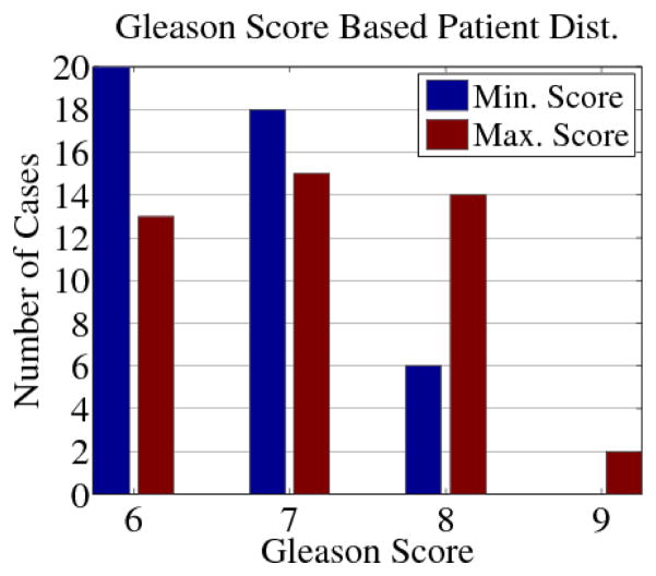
The cohort had biopsy Gleason scores ranging from (3+3) to (4+5) with the patient distribution according to each case’s smallest and largest scores shown in Fig. 5. Biopsies containing a Gleason score above or equal to (4+4) were classified as aggressive cases as the ground truth criterion, which is a standard practice in the literature [11], [22]. The analysis was carried out following the steps of Section 3, as exemplified by Figs. 7 and 8.

Figure 5.

Distribution of the cohort based on patient smallest (blue) and largest (red) Gleason Scores. One (4+5) patient had a (4+4) core as the smallest score.

The retrospective analysis with InFS–Explorer^© revealed a potential biomarker in the form of a specific region within MR–FS [48], namely a bulge in [low ADC]–[mid–low T2W], for distinguishing aggressive from indolent PCa (see Fig. 6).

Within the cohort, one aggressive and two low–risk cases (not shown) were declared inconclusive. The aggressive case was considered as a false negative for analysis purposes. In another aggressive case (not shown), the anatomic loci corresponding to the encapsulated MR–FS bulge covered less than the tumor burden observed in T2W images. However, this is expected since PCas are notoriously heterogeneous and may contain both aggressive and less aggressive regions as shown in Fig. 8. Reciprocally, the demarcation of the anatomic burden engaged a small portion of the MR-FS bulge with most of the features leaning towards the center of the FS. Nevertheless, despite the discovery of motion artifacts in T2W images, this case was declared a false negative as well.

The only false positive case, shown in Fig. 3, displayed an FS bulge with Gleason scores from midline apical mid anterior central axial and sagittal sampling reporting (3+3) 80% and (3+4) 60%, and midline mid base anterior central axial and sagittal (3+4) 6% and (3+3) 50%, all involving 1 biopsy core. In this case, the biopsy scores have been validated by the post–prostatectomy histopathology (written) report.

In all of the cases, demarcation of MR–FS ROIs in the [low ADC]–[low T2W] range resulted in benign anatomic loci, such as the anterior fibrous stroma, various prostatic capsule regions and pseudocapsule. This important observation further validates potential location of features of aggressiveness in the [low ADC]–[mid–low T2W] region.

Moreover, the FS ROIs of Figs. 7 and 8, with oblique edges and the non–convex polygon of Fig. 8 demonstrate that one sided or range based thresholding (see Fig. 9), and more generally any method producing convex FS ROIs might incorporate false positive malignant pixels (see the green arrow in Fig. 8). This motivates a preference for nonlinear pattern recognition algorithms (e.g., over linear SVMs) in the future.

Figure 9.

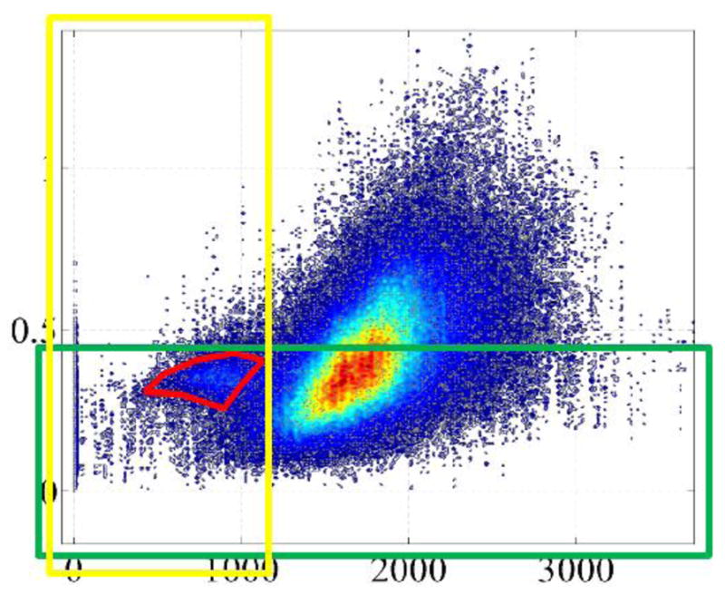
Individual or combination range thresholding shown as yellow and green boxes cannot capture the non–convex malignant region thereby resulting in many false negative feature points (see also [49]).

In conclusion, agreement with cohort biopsy findings provides evidence that a specific region of FS corresponding to low ADC–mid–low T2W yields aggressive PCa with high confidence as summarized by the Table 1. In addition to motivating careful future investigations for further verification towards a complete validation (e.g., by full mount histopathology), herein, valuable biophysical information was obtained by exploring T2W–ADC MR–FS properties with InFS–Explorer^©.

Table 1.

The Performance of the Binary Classification Test of Aggressiveness on the Cohort

True Positive	False Positive	Positive Predictive
13	1	0.929
False Negative	True Negative	Negative Predictive
2	28	0.933
Sensitivity	Specificity
0.867	0.965

5 Preliminary Results on Renal Cell Carcinoma

Renal cortical tumors are a family of neoplasms with different biological features and clinical behavior creating significant challenges in disease identification. With the increase of incidental detection [50], postoperative evidence suggests that a significant portion of renal lesions that are falsely diagnosed as malignant are eventually proven benign after pathological examination [51]. The insufficiency of existing imaging and biopsy techniques to accurately diagnose and identify disease subtypes is a significant concern towards the aim of avoiding unnecessary interventions. Consequently, improvements could potentially be achieved by the use of multi–modal imaging with the InFS–Explorer^© platform.

Herein, preliminary investigations were conducted using the two sub–modalities of MRI Chemical Shift Imaging (CSI) [52]. The FS was formed by using {Out–Phase, In–Phase} CSI characteristics obtained by changing the echo time (TE). Whereas in In–Phase images both water and lipid magnetic moments are aligned at the echo time to create a strong signal, the opposite occurs for the Out–Phase portion, thereby creating signal strength differences between water and lipid protons at each location [52].

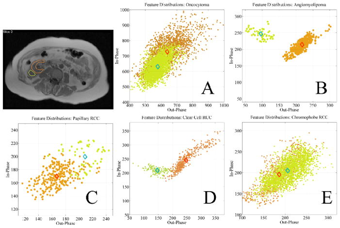
In the past, CSI has been investigated to quantify lipid content of renal cortical tumors, which could be a differentiating factor [53], [54]. A recent study showed marked CSI differences in angiomyolipomas and clear cell renal cell carcinomas (RCC), but lesser degrees of CSI differentiability was also noted in oncocytomas and, papillary and chromophobe RCCs [55]. Such studies are based on visually selected anatomical ROI analysis by different observers, which inevitably creates variability between their evaluations. In order to address this challenge, InFS–Explorer^© was used on the MR–FS of renal cancer cases. The outcome is highly encouraging towards future studies with inclusion of different biomedical imaging modality combinations, such as utilization of dynamic contrast enhanced (DCE) MRI and DWI.

Data from five patients with different renal cancer subtypes (see Fig. 10 and Table 2) admitted to Memorial Sloan–Kettering Cancer Center were analyzed. As both image sets were at the same resolution, there was not a need for co–registration. A 1.5T GE Signa Excite MR scanner with TR/TE(in)/TE(out) = 185/4.509/2.216 ms, slice thickness 8 mm, flip angle 90°, 8 channel body upper receive coil, 256×256 resolution were used in data collection.

Figure 10.

Feature vectors based on CSI characteristics defined by ROI analysis of the anatomical images in five different types of renal cortical tumors. FS neighborhoods of tumor (green) and normal renal cortex (orange) are very similar for oncocytoma (A), papillary RCC (C), and chromophobe RCC (E), whereas FS neighborhoods of tumor (green) and normal renal cortex (orange) are markedly separated in angiomyolipoma (B) and clear cell RCC (D) due to their unique CSI characteristics.

Table 2.

Feature Cloud Center Separation for Renal Cancer Types

Oncocytoma	Angiom.	Papillary	Clear Cell	Chromo.
0.11638	0.41386	0.21533	0.30957	0.08362

In each patient anatomic regions from the renal cortex and the tumor area were demarcated with InFS–Explorer^© to observe corresponding features (see Fig 10) by a radiologist. The separation of the features was quantified using the normalized distances between feature cloud centers (diamonds in Fig. 10) in Table 2. The Euclidean norm of the center of renal cortex feature cloud was used as the distance normalization factor.

In comparison to angiomyolipoma and clear cell RCC, the results showed a lesser degree of lipid content difference between the renal cortex and tumor sites for oncocytoma, chromophobe RCC and, papillary RCC as seen in Fig. 10.

This analysis is in accordance with previous observations of marked differences in CSI characteristics of angiomyolipomas and clear cell RCCs compared to other renal cortical tumors. Furthermore, as previous studies were limited by visual analysis of tumor ROIs that is subject to observer bias, this study underlines the potential advantages of analyzing and depicting CSI data on MR–FS, which allows robust and quantitative analysis of renal cortical tumors.

In conclusion, for this preliminary cohort of 5 patients, MR–FS analysis of renal cortical tumors based on their CSI characteristics with marked separation of their feature vector clouds shows potential for future differentiation of angiomyolipoma and clear cell RCC.

6 Conclusion and Future Directions

In this paper, a working prototype of InFS–Explorer^© has been introduced as a computer aided decision and exploration tool for interactive multi–modal imaging data analysis. InFS–Explorer^© is a transparent tool that allows direct examination of tissue properties elucidated by multi–modal biomedical imaging.

The platform’s utility has been demonstrated in two institutions for two different purposes with two different pathologies, prostate and renal cancer, showing promise. In both cases, InFS–Explorer^© analysis provided valuable biophysical information, which does not occur with automated algorithms.

While the paper achieved the proof of concept from an engineering standpoint, findings on PCa and renal cancer data are not mature enough to be clinically significant yet. Dedicated studies including larger and possibly multi–institutional cohorts with more detailed ground truth information, such as full mount histopathology, will be conducted in the future. For PCa, these will provide a strong cross–validation and ensure the proposed biomarker’s robustness.

Unlike modification requirements of specific automatic algorithms for new pathologies, e.g., redesign for PCa starting from breast, lung and colorectal cancer and, retinal imaging (see the references in [40], [11]), InFS–Explorer^© is readily compatible with distinct circumstances. Accordingly, the platform will be tested in the future with other cancer types in different organs, e.g., glioblastomas, as well as with neurological diseases and disorders, such as multiple sclerosis.

In practice, computer aided systems are not meant to replace the physicians, but are merely tools for assisting them, e.g., automatic algorithms aiming to improve observer performance [38]. InFS–Explorer^© is based on the presence of physicians in–the–loop, which already occurs during algorithm development. In addition to potentially improving ground truth determination, the platform’s manual evaluation capability becomes more relevant especially for outlier cases or when automated algorithms are inconclusive. Similarly, when evaluating complex pathologies like the PCa in this work, direct visual inspection of FS alone proved to be insufficient. Mainly, because of the potential biomarker’s appearance at varying locations and its diverse shapes (see Figs. 7 and 8) manual investigations were necessary for locating malignant ROIs.

More generally, extraction of relevant information from standard imaging data leads to potential improvements in the accuracy of clinical decisions with potential reduction in health care costs while providing optimal individualized care. For example, accurately locating aggressive tumor burden with InFS–Explorer^©, could improve the accuracy of biopsies and radiation therapy guidance while decreasing the time needed for interpretation. Accordingly, in scenarios where rapid decisions are needed, such as image guided robotic interventions, incorporation of InFS–Explorer^© within the interventional device’s command and control platform [56] might be advantageous.

Moreover, during surveillance, observing the changes in the MR–FS in a single instance can be more time efficient than evaluating a large number of images longitudinally. Rather than attempting to reach a consensus about the malignant loci at multiple images, which is potentially more susceptible to variability, identification with a single agreement on the FS region boundary (see, Fig. 11) may reduce inter– and intra–observer variability. The significance of this increases when faced with tumor heterogeneity, which is recognized histologically but not yet fully appreciated in biomedical images. Consequently, future plans include testing this variability reduction hypothesis with dedicated multi–reader studies.

Figure 11.

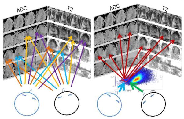
Potentially, by deciding on a single malignant ROI within the FS on the right, rather than regions in multiple images on the left, observer variability might be reduced.

Finally, the prototype platform introduced herein operates on 2 –dimensional FSs, where easily selecting ROIs is possible. Combining additional modalities would definitely be more beneficial for enlarging the multi–modal information pool. However, increasing the FS dimensions beyond 3 creates perception limitations for manually demarcating hyper–volumes of interest. Developing new visualization methods and/or dimension reduction techniques will be necessary for the future achievement of this goal.

References

- 1.Ciccarelli O, Catani M, Johansen-Berg H, Clark C, Thompson A. Diffusion–based tractography in neurological disorders: concepts, applications, and future developments. The Lancet Neurology. 2008;7(8):715–727. doi: 10.1016/S1474-4422(08)70163-7. [DOI] [PubMed] [Google Scholar]
- 2.Mac Donald CL, Johnson AM, Cooper D, Nelson EC, Werner NJ, Shimony JS, Snyder AZ, Raichle ME, Witherow JR, Fang R, Flaherty SF, Brody DL. Detection of blast–related traumatic brain injury in U.S. military personnel. New England Journal of Medicine. 2011;364(22):2091–2100. doi: 10.1056/NEJMoa1008069. http://www.nejm.org/doi/full/10.1056/NEJMoa1008069. [DOI] [PMC free article] [PubMed] [Google Scholar]
- 3.Sati P, van Gelderen P, Silva AC, Reich DS, Merkle H, de Zwart JA, Duyn JH. Micro–compartment specific relaxation in the brain. NeuroImage. 2013;77:268–278. doi: 10.1016/j.neuroimage.2013.03.005. http://www.sciencedirect.com/science/article/pii/S1053811913002139. [DOI] [PMC free article] [PubMed] [Google Scholar]
- 4.Turkbey B, Albert PS, Kurdziel K, Choyke PL. Imaging localized prostate cancer: Current approaches and new developments. American Journal of Roentgenology. 2009;192(6):1471–1480. doi: 10.2214/AJR.09.2527. http://www.ajronline.org/content/192/6/1471.abstract. [DOI] [PMC free article] [PubMed] [Google Scholar]
- 5.Turkbey B, Choyke PL. Multiparametric MRI and prostate cancer diagnosis and risk stratification. Current Opinion in Urology. 2012;22(4):310–315. doi: 10.1097/MOU.0b013e32835481c2. [DOI] [PMC free article] [PubMed] [Google Scholar]
- 6.Lim HK, Kim JK, Kim KA, Cho KS. Prostate cancer: Apparent diffusion coefficient map with T2-weighted images for detection–a multireader study. Radiology. 2009;250(1):145–151. doi: 10.1148/radiol.2501080207. http://dx.doi.org/10.1148/radiol.2501080207. [DOI] [PubMed] [Google Scholar]
- 7.Donati OF, Afaq A, Vargas HA, Mazaheri Y, Zheng J, Moskowitz CS, Hricak H, Akin O. Prostate MRI: Evaluating tumor volume and apparent diffusion coefficient as surrogate biomarkers for predicting tumor gleason score. Clinical Cancer Research. 2014;20(14):3705–3711. doi: 10.1158/1078-0432.CCR-14-0044. http://clincancerres.aacrjournals.org/content/20/14/3705.abstract. [DOI] [PubMed] [Google Scholar]
- 8.Singer EA, Kaushal A, Turkbey B, Couvillon A, Pinto PA, Parnes HL. Active surveillance for prostate cancer: past, present and future. Current Opinion in Oncology. 2012;24(3):243–250. doi: 10.1097/CCO.0b013e3283527f99. [DOI] [PMC free article] [PubMed] [Google Scholar]
- 9.Wassberg C, Akin O, Vargas HA, Shukla-Dave A, Zhang J, Hricak H. The incremental value of contrast-enhanced MRI in the detection of biopsy-proven local recurrence of prostate cancer after radical prostatectomy: Effect of reader experience. American Journal of Roentgenology. 2012;199(2):360–366. doi: 10.2214/AJR.11.6923. [DOI] [PMC free article] [PubMed] [Google Scholar]
- 10.Fütterer JJ, Heijmink SWTPJ, Scheenen TWJ, Jager GJ, Hulsbergen-Van de Kaa CA, Witjes JA, Barentsz JO. Prostate cancer: Local staging at 3–T endorectal MR imaging–early experience. Radiology. 2006;238(1):184–191. doi: 10.1148/radiol.2381041832. http://dx.doi.org/10.1148/radiol.2381041832. [DOI] [PubMed] [Google Scholar]
- 11.Vos PC, Barentsz JO, Karssemeijer N, Huisman HJ. Automatic computer–aided detection of prostate cancer based on multiparametric magnetic resonance image analysis. Physics in Medicine and Biology. 2012;57(6):1527. doi: 10.1088/0031-9155/57/6/1527. http://stacks.iop.org/0031-9155/57/i=6/a=1527. [DOI] [PubMed] [Google Scholar]
- 12.Litjens G, Debats O, Barentsz J, Karssemeijer N, Huisman H. Computer–aided detection of prostate cancer in MRI, Medical Imaging. IEEE Transactions on. 2014;33(5):1083–1092. doi: 10.1109/TMI.2014.2303821. [DOI] [PubMed] [Google Scholar]
- 13.Yu J, Fulcher AS, Turner MA, Cockrell CH, Cote EP, Wallace TJ. Prostate cancer and its mimics at multiparametric prostate MRI. The British Journal of Radiology. 2014;87(1037):20130659. doi: 10.1259/bjr.20130659. http://dx.doi.org/10.1259/bjr.20130659. [DOI] [PMC free article] [PubMed] [Google Scholar]
- 14.Vapnik VN. Statistical learning theory, Adaptive and learning systems for signal processing, communications, and control. Wiley; New York: 1998. [Google Scholar]
- 15.Cristianini N, Shaw-Taylor J. An Introduction to Support Vector Macines and Other Kernel–Based Learning Methods. Cambridge University Press; New York, USA: 2000. [Google Scholar]
- 16.Duda RO, Hart PE, Stork DG. Pattern Classification. 2. Wiley-Interscience; New York: 2000. [Google Scholar]
- 17.Vannier MW, Butterfield RL, Jordan D, Murphy WA, Levitt RG, Gado M. Multispectral analysis of magnetic resonance images. Radiology. 1985;154(1):221–224. doi: 10.1148/radiology.154.1.3964938. http://pubs.rsna.org/doi/abs/10.1148/radiology.154.1.3964938. [DOI] [PubMed] [Google Scholar]
- 18.Clarke L, Velthuizen R, Camacho M, Heine J, Vaidyanathan M, Hall L, Thatcher R, Silbiger M. MRI segmentation: Methods and applications. Magnetic Resonance Imaging. 1995;13(3):343–368. doi: 10.1016/0730-725x(94)00124-l. http://dx.doi.org/10.1016/0730-725X(94)00124-L http://www.sciencedirect.com/science/article/pii/0730725X9400124L. [DOI] [PubMed] [Google Scholar]
- 19.Vovk U, Pernus F, Likar B. A review of methods for correction of intensity inhomogeneity in MRI, Medical Imaging. IEEE Transactions on. 2007;26(3):405–421. doi: 10.1109/TMI.2006.891486. [DOI] [PubMed] [Google Scholar]
- 20.Soltanian-Zadeh H, Windham J, Peck D. Optimal linear transformation for MRI feature extraction, Medical Imaging. IEEE Transactions on. 1996;15(6):749–767. doi: 10.1109/42.544494. [DOI] [PubMed] [Google Scholar]
- 21.Moradi M, Salcudean SE, Chang SD, Jones EC, Buchan N, Casey RG, Goldenberg SL, Kozlowski P. Multiparametric MRI maps for detection and grading of dominant prostate tumors. Journal of Magnetic Resonance Imaging. 2012;35(6):1403–1413. doi: 10.1002/jmri.23540. http://dx.doi.org/10.1002/jmri.23540. [DOI] [PMC free article] [PubMed] [Google Scholar]
- 22.Delongchamps NB, Rouanne M, Flam T, Beuvon F, Liberatore M, Zerbib M, Cornud F. Multiparametric magnetic resonance imaging for the detection and localization of prostate cancer: combination of T2–weighted, dynamic contrast–enhanced and diffusion–weighted imaging. BJU International. 2011;107(9):1411–1418. doi: 10.1111/j.1464-410X.2010.09808.x. http://dx.doi.org/10.1111/j.1464-410X.2010.09808.x. [DOI] [PubMed] [Google Scholar]
- 23.MathWorks, Natick, MA, USA. Matlab Manual: Mathematics. 2014 Mar; http://www.mathworks.com/help/matlab/index.html.
- 24.Vos PC, Hambrock T, Barenstz JO, Huisman HJ. Computer-assisted analysis of peripheral zone prostate lesions using T2–weighted and dynamic contrast enhanced T1–weighted MRI. Physics in Medicine and Biology. 2010;55(6):1719–1734. doi: 10.1088/0031-9155/55/6/012. http://stacks.iop.org/0031-9155/55/i=6/a=012. [DOI] [PubMed] [Google Scholar]
- 25.Niaf E, Rouvière O, Mège-Lechevallier F, Bratan F, Lartizien C. Computer–aided diagnosis of prostate cancer in the peripheral zone using multiparametric MRI. Physics in Medicine and Biology. 2012;57(12):3833. doi: 10.1088/0031-9155/57/12/3833. http://stacks.iop.org/0031-9155/57/i=12/a=3833. [DOI] [PubMed] [Google Scholar]
- 26.Franklin WR. [accessed 16-September-2014];Pnpoly – point inclusion in polygon test. 2014 Online http://www.ecse.rpi.edu/wrf/Research/Short_Notes/pnpoly.html.
- 27.O’Rourke J. Computational Geometry in C. 2. Cambridge University Press; 1998. cambridge Books Online http://dx.doi.org/10.1017/CBO9780511804120. [Google Scholar]
- 28.Siegel R, Naishadham D, Jemal A. Cancer statistics, 2013. CA: A Cancer Journal for Clinicians. 2013;63(1):11–30. doi: 10.3322/caac.21166. http://dx.doi.org/10.3322/caac.21166. [DOI] [PubMed] [Google Scholar]
- 29.Hugosson J, Carlsson S, Aus G, Bergdahl S, Khatami A, Lodding P, Pihl CG, Stranne J, Holmberg E, Lilja H. Mortality results from the Göteborg randomised population-based prostate-cancer screening trial. The Lancet Oncology. 2010;11(8):725–732. doi: 10.1016/S1470-2045(10)70146-7. http://www.sciencedirect.com/science/article/pii/S1470204510701467. [DOI] [PMC free article] [PubMed] [Google Scholar]
- 30.Levine MA, Ittman M, Melamed J, Lepor H. Two consecutive sets of transrectal ultrasound guided sextant biopsies of the prostate for the detection of prostate cancer. The Journal of Urology. 1998;159(2):471–476. doi: 10.1016/S0022-5347(01)63951-X. http://www.sciencedirect.com/science/article/pii/S002253470163951X. [DOI] [PubMed] [Google Scholar]
- 31.Sciarra A, Barentsz J, Bjartell A, Eastham J, Hricak H, Panebianco V, Witjes JA. Advances in magnetic resonance imaging: How they are changing the management of prostate cancer. European Urology. 2011;59(6):962–977. doi: 10.1016/j.eururo.2011.02.034. http://www.sciencedirect.com/science/article/pii/S0302283811001667. [DOI] [PubMed] [Google Scholar]
- 32.Mazaheri Y, Shukla-Dave A, Muellner A, Hricak H. MRI of the prostate: Clinical relevance and emerging applications. Journal of Magnetic Resonance Imaging. 2011;33(2):258–274. doi: 10.1002/jmri.22420. http://dx.doi.org/10.1002/jmri.22420. [DOI] [PubMed] [Google Scholar]
- 33.Oto A, Kayhan A, Jiang Y, Tretiakova M, Yang C, Antic T, Dahi F, Shalhav AL, Karczmar G, Stadler WM. Prostate cancer: Differentiation of central gland cancer from benign prostatic hyperplasia by using diffusion–weighted and dynamic contrast-enhanced MR imaging. Radiology. 2010;257(3):715–723. doi: 10.1148/radiol.10100021. http://radiology.rsna.org/content/257/3/715.abstract. [DOI] [PMC free article] [PubMed] [Google Scholar]
- 34.Akin O, Sala E, Moskowitz CS, Kuroiwa K, Ishill NM, Pucar D, Scardino PT, Hricak H. Transition zone prostate cancers: Features, detection, localization, and staging at endorectal MR imaging. Radiology. 2006 Jun;239(3):784–792. doi: 10.1148/radiol.2392050949. http://radiology.rsna.org/content/239/3/784.abstract. [DOI] [PubMed] [Google Scholar]
- 35.Yacoub JH, Oto A, Miller FH. MR imaging of the prostate. Radiologic Clinics of North America. 2014;52(4):811–837. doi: 10.1016/j.rcl.2014.02.010. adult Body MR http://dx.doi.org/10.1016/j.rcl.2014.02.010 http://www.sciencedirect.com/science/article/pii/S003383891400027X. [DOI] [PubMed] [Google Scholar]
- 36.Johnson LM, Turkbey B, Figg WD, Choyke PL. Multiparametric MRI in prostate cancer management. Nat Rev Clin Oncol. 2014;11(6):346–353. doi: 10.1038/nrclinonc.2014.69. [DOI] [PMC free article] [PubMed] [Google Scholar]
- 37.Durmus T, Baur A, Hamm B. Multiparametric magnetic resonance imaging in the detection of prostate cancer. Fortschr Röntgenstr. 2014;186(03):238–246. doi: 10.1055/s-0034-1365937. [DOI] [PubMed] [Google Scholar]
- 38.Hambrock T, Vos PC, Hulsbergen-van de Kaa CA, Barentsz JO, Huisman HJ. Prostate cancer: Computer–aided diagnosis with multiparametric 3-T MR imaging–effect on observer performance. Radiology. 2013;266(2):521–530. doi: 10.1148/radiol.12111634. http://dx.doi.org/10.1148/radiol.12111634. [DOI] [PubMed] [Google Scholar]
- 39.Chan I, WW, Mulkern RV, Haker S, Zhang J, Zou KH, Maier SE, Tempany CMC. Detection of prostate cancer by integration of line–scan diffusion, T2-mapping and T2-weighted magnetic resonance imaging; a multichannel statistical classifier. Medical Physics. 2003;30(9):2390–2398. doi: 10.1118/1.1593633. http://link.aip.org/link/?MPH/30/2390/1. [DOI] [PubMed] [Google Scholar]
- 40.Peng Y, Jiang Y, Yang C, Brown JB, Antic T, Sethi I, Schmid-Tannwald C, Giger ML, Eggener SE, Oto A. Quantitative analysis of multiparametric prostate MR images: Differentiation between prostate cancer and normal tissue and correlation with gleason score—-a computer–aided diagnosis development study. Radiology. 2013;267(3):787–796. doi: 10.1148/radiol.13121454. http://dx.doi.org/10.1148/radiol.13121454. [DOI] [PMC free article] [PubMed] [Google Scholar]
- 41.Artan Y, Haider M, Langer D, van der Kwast T, Evans A, Yang Y, Wernick M, Trachtenberg J, Yetik I. Prostate cancer localization with multispectral MRI using cost–sensitive support vector machines and conditional random fields, Image Processing. IEEE Transactions on. 2010;19(9):2444–2455. doi: 10.1109/TIP.2010.2048612. [DOI] [PubMed] [Google Scholar]
- 42.Ozer S, Langer DL, Liu X, Haider MA, van der Kwast TH, Evans AJ, Yang Y, Wernick MN, Yetik IS. Supervised and unsupervised methods for prostate cancer segmentation with multispectral MRI. Medical Physics. 2010;37(4):1873–1883. doi: 10.1118/1.3359459. http://link.aip.org/link/?MPH/37/1873/1. [DOI] [PubMed] [Google Scholar]
- 43.Tiwari P, Kurhanewicz J, Madabhushi A. Multi-kernel graph embedding for detection, gleason grading of prostate cancer via MRI/MRS. Medical Image Analysis. 2013;17(2):219–235. doi: 10.1016/j.media.2012.10.004. http://dx.doi.org/10.1016/j.media.2012.10.004 http://www.sciencedirect.com/science/article/pii/S1361841512001491. [DOI] [PMC free article] [PubMed] [Google Scholar]
- 44.Tretiakova M, Antic T, Binder D, Kocherginsky M, Liao C, Taxy JB, Oto A. Microvessel density is not increased in prostate cancer: digital imaging of routine sections and tissue microarrays. Human Pathology. 2013;44(4):495–502. doi: 10.1016/j.humpath.2012.06.009. http://dx.doi.org/10.1016/j.humpath.2012.06.009 http://www.sciencedirect.com/science/article/pii/S0046817712002286. [DOI] [PubMed] [Google Scholar]
- 45.Song SK, Qu Z, Garabedian EM, Gordon JI, Milbrandt J, Ackerman JJH. Improved magnetic resonance imaging detection of prostate cancer in a transgenic mouse model. Cancer Research. 2002;62(5):1555–1558. http://cancerres.aacrjournals.org/content/62/5/1555.abstract. [PubMed] [Google Scholar]
- 46.Fotin SV, Yin Y, Periaswamy S, Kunz J, Haldankar H, Muradyan N, Cornud F, Turkbey B, Choyke PL. Normalized gradient fields cross–correlation for automated detection of prostate in magnetic resonance images. Proc SPIE. 2012;8314:83140V–83140V–11. doi: 10.1117/12.911620. http://dx.doi.org/10.1117/12.911620. [DOI] [Google Scholar]
- 47.Turkbey B, Fotin SV, Huang RJ, Yin Y, Daar D, Aras O, Bernardo M, Garvey BE, Weaver J, Haldankar H, Muradyan N, Merino MJ, Pinto PA, Periaswamy S, Choyke PL. Fully automated prostate segmentation on MRI: Comparison with manual segmentation methods and specimen volumes. American Journal of Roentgenology. 2013;201(5):W720–W729. doi: 10.2214/AJR.12.9712. [DOI] [PubMed] [Google Scholar]
- 48.Özcan A, Türkbey B, Choyke PL, Mun SK. Aggressiveness biomarker for prostate cancer in ADC–T2W MR feature space. Proceedings of the Joint Annual Meeting ISMRM–ESMRB; 2014; Milan, Italy: ISMRM; 2014. p. 1076. [Google Scholar]
- 49.Bonar DC, Schaper KA, Anderson JR, Rottenberg DA, Strother SC. Graphical analysis of MR feature space for measurement of CSF, gray–matter, and white–matter volumes. Journal of Computer Assisted Tomography. 1993;17(3):461–470. doi: 10.1097/00004728-199305000-00024. [DOI] [PubMed] [Google Scholar]
- 50.Lane BR, Babineau DC, Poggio ED, Weight CJ, Larson BT, Gill IS, Novick AC. Factors predicting renal functional outcome after partial nephrectomy. The Journal of Urology. 2008;180(6):2363–2369. doi: 10.1016/j.juro.2008.08.036. http://dx.doi.org/10.1016/j.juro.2008.08.036 http://www.sciencedirect.com/science/article/pii/S0022534708021617. [DOI] [PubMed] [Google Scholar]
- 51.Corcoran AT, Russo P, Lowrance WT, Asnis-Alibozek A, Libertino JA, Pryma DA, Divgi CR, Uzzo RG. A review of contemporary data on surgically resected renal masses–benign or malignant? Urology. 2013;81(4):707–713. doi: 10.1016/j.urology.2013.01.009. http://dx.doi.org/10.1016/j.urology.2013.01.009 http://www.sciencedirect.com/science/article/pii/S0090429513000320. [DOI] [PubMed] [Google Scholar]
- 52.Buxton RB, Wismer GL, Brady TJ, Rosen BR. Quantitative proton chemical-shift imaging. Magnetic Resonance in Medicine. 1986;3(6):881–900. doi: 10.1002/mrm.1910030609. http://dx.doi.org/10.1002/mrm.1910030609. [DOI] [PubMed] [Google Scholar]
- 53.Yoshimitsu K, Honda H, Kuroiwa T, Irie H, Tajima T, Jimi M, Kuroiwa K, Naito S, Masuda K. MR detection of cytoplasmic fat in clear cell renal cell carcinoma utilizing chemical shift gradient–echo imaging. Journal of Magnetic Resonance Imaging. 1999;9(4):579–585. doi: 10.1002/(sici)1522-2586(199904)9:4<579::aid-jmri12>3.0.co;2-s. [DOI] [PubMed] [Google Scholar]
- 54.Outwater EK, Bhatia M, Siegelman ES, Burke MA, Mitchell DG. Lipid in renal clear cell carcinoma: detection on opposed–phase gradient–echo MR images. Radiology. 1997;205(1):103–107. doi: 10.1148/radiology.205.1.9314970. http://pubs.rsna.org/doi/abs/10.1148/radiology.205.1.9314970. [DOI] [PubMed] [Google Scholar]
- 55.Karlo C, Donati O, Burger I, Zheng J, Moskowitz C, Hricak H, Akin O. MR imaging of renal cortical tumours: qualitative and quantitative chemical shift imaging parameters. European Radiology. 2013;23(6):1738–1744. doi: 10.1007/s00330-012-2758-x. http://dx.doi.org/10.1007/s00330-012-2758-x. [DOI] [PubMed] [Google Scholar]
- 56.Özcan A, Tsekos NV. The interconnection of MRI scanner and MR compatible robotic device: Synergistic graphical user interface to form a mechatronic system. IEEE/ASME Transactions on Mechatronics. 2008;13(3):362–369. doi: 10.1109/TMECH.2008.924120. [DOI] [PMC free article] [PubMed] [Google Scholar]