

Abstract
The extent to which socioeconomic (dis)advantage is transmitted between generations is receiving increasing attention from academics and policymakers. However, few studies have investigated whether there is a spatial dimension to this intergenerational transmission of (dis)advantage. Drawing on the concept of neighbourhood biographies, this study contends that there are links between the places individuals live with their parents and their subsequent neighbourhood experiences as independent adults. Using individual-level register data tracking the whole Stockholm population from 1990 to 2008, and bespoke neighbourhoods, this study is the first to use sequencing techniques to construct individual neighbourhood histories. Through visualisation methods and ordered logit models, we demonstrate that the socioeconomic composition of the neighbourhood children lived in before they left the parental home is strongly related to the status of the neighbourhood they live in 5, 12 and 18 years later. Children living with their parents in high poverty concentration neighbourhoods are very likely to end up in similar neighbourhoods much later in life. The parental neighbourhood is also important in predicting the cumulative exposure to poverty concentration neighbourhoods over a long period of early adulthood. Ethnic minorities were found to have the longest cumulative exposure to poverty concentration neighbourhoods. These findings imply that for some groups, disadvantage is both inherited and highly persistent.
Keywords: intergenerational transmission, deprived neighbourhoods, neighbourhood biography, sequence analysis, Sweden
Introduction
There is a large body of literature investigating the intergenerational transmission of (dis)advantage. It has long been recognised that ‘the fortunes of children are linked to their parents’ (Becker and Tomes 1979, 1153), and it is now well established that individual characteristics, such as labour market earnings and educational attainment, correlate strongly between parents and children (D'Addio 2007). The extent to which socioeconomic (dis)advantage is transmitted between generations is receiving increasing attention from policymakers. According to the UK government report Opening doors, breaking barriers: a strategy for social mobility,
In Britain today, life chances are narrowed for too many by the circumstances of their birth: the home they're born into, the neighbourhood they grow up in or the jobs their parents do. Patterns of inequality are imprinted from one generation to the next. (Nick Clegg, Cabinet Office 2011)
This liberal belief in the importance of severing the links between ascribed or inherited characteristics and individual attainment has become an important policy objective across the developed world, advocated for both equity and efficiency reasons (OECD 2010).
It has been suggested – sometimes implicitly – that the intergenerational transmission of (dis)advantage also has a spatial dimension (Duncan and Raudenbush 2001; Jencks and Mayer 1990; Sampson and Wilson 1995; van Ham et al. 2012). The idea is that children who grow up in poverty concentration neighbourhoods might be more likely than others to end up in such a neighbourhood as adults. To our knowledge there is only one study to date that empirically investigates this spatial dimension (see Vartanian et al. 2007).
The possibility of a spatial dimension to intergenerational transmission of (dis)advantage is highly relevant for the literature on neighbourhood effects. This literature investigates whether living in a poverty concentration neighbourhood (see Wilson 1987) has a negative effect on residents’ life chances (related to, for example, income, education and health), over and above the effect of their individual characteristics (see Ellen and Turner 1997; Galster 2002; Manley and van Ham 2012). Despite an enormous and growing body of literature on neighbourhood effects, there is little agreement on the causal mechanisms that might produce them, their relative importance compared with individual characteristics, and under which circumstances and where these effects are important (van Ham et al. 2012). A major problem in identifying causal neighbourhood effects is that people do not randomly select their neighbourhoods, and as a result parameter estimates for these effects are biased (Durlauf 2004; van Ham and Manley 2010). This process of neighbourhood selection, which over the life course cumulatively creates an individual's neighbourhood biography, may be influenced by the parental neighbourhood. Consequently, individual life outcomes might not only be related to the current neighbourhood, but also to neighbourhood histories.
Insight into the neighbourhood histories of individuals will not only benefit the literature on neighbourhood effects, but will also contribute to our understanding of both segregation and residential mobility processes. Many studies of residential mobility use the life course approach as a starting point and analyse longitudinal data, but few studies investigate true life courses empirically as they only investigate transitions in states between two years (e.g. Rabe and Taylor 2010). As a result, very little is known about the wider neighbourhood biographies within which these events and transitions are situated. This is problematic, as the biographical context within which an event occurs can condition its significance and meaning (Coulter and van Ham forthcoming; Dykstra and van Wissen 1999). For example, a move from an affluent neighbourhood to a poverty concentration neighbourhood has a very different meaning depending on whether the stay in this poor neighbourhood is temporary or more permanent.
This is the first paper to construct the entire neighbourhood histories of a large group of individuals over a long period of time. We investigated the intergenerational transmission of neighbourhood poverty in Stockholm through the effect of the parental neighbourhood on individual neighbourhood biographies over a period of almost two decades. This study hypothesised that the parental neighbourhood has predictive value for neighbourhood outcomes later in life and for the cumulative exposure to poverty concentration neighbourhoods over the life course. To relate the neighbourhood careers of parental home leavers in the Stockholm metropolitan area to the last neighbourhood they lived in with their parents, we used 1990–2008 longitudinal register data from the GeoSweden database. We defined poverty concentration neighbourhoods based on the percentage of low-income neighbours in the local area. We used bespoke neighbourhoods based on the characteristics of the 500 people living closest to each individual (Östh et al. forthcoming) and used innovative sequencing techniques to visualise individual neighbourhood histories (for a residential mobility application see Coulter and van Ham forthcoming). Sweden provides an excellent case study for the analysis of the intergenerational transmission of neighbourhood characteristics, because despite evidence for increasing social polarisation (Hedin et al. 2012), Sweden is widely considered to be one of the least stratified Western societies (on the nature of welfare states in Western societies see Esping-Andersen 1990). As a result, this study provides an important counterweight to studies on US and British societies that dominate the segregation literature (Maloutas 2012).
Literature review
To link our understanding of residential mobility (histories) and neighbourhood choice to the literature on intergenerational transmission of (dis)advantage, this study adopts the life course approach as used in many residential mobility studies (Clark and Huang 2003). In contrast with the more normative and deterministic life cycle approach, life course theory argues that individuals experience their own unique sequence of life events as they age (Clark and Dieleman 1996; Geist and McManus 2008; van Ham 2012). As a result, individual lives can be thought of as unique personal biographies (Dykstra and van Wissen 1999; Elder 1994). Mulder and Hooimeijer (1999) argue that the life events occurring within these personal biographies can be grouped into four parallel life course careers. In this framework, it is the sequence of events experienced in these interlinking household, labour force, education and housing careers that influence an individual's residential mobility behaviour throughout their lifetime (Clark and Withers 2007). Crucially, the life course model posits that an individual's choices and behaviours can be strongly affected by the events or states they have experienced earlier in their life (Dykstra and van Wissen 1999; Feijten 2005; Feijten et al. 2008). Adopting a life course approach therefore guides researchers to analyse the occurrence of events within the long-term individual biography and macro-context within which these are situated (Aisenbrey and Fasang 2010).
While the evolution of housing careers across the life course has been a focus for much housing and mobility research (Clark et al. 2003; Feijten and Mulder 2005), most studies have been based around the empirical analysis of either cross-sectional data containing some retrospective information, or short periods of longitudinal data (e.g. Clark and Ledwith 2006; Geist and McManus 2008). The result is a focus on year-to-year mobility instead of mobility biographies over the life course. Such studies typically show that households often move between dwellings to adjust their space consumption in response to their changing household needs (Clark and Dieleman 1996; Clark and Huang 2003). Changes in household composition are also often associated with moves to different types of dwellings in different types of neighbourhoods (Mulder and Hooimeijer 1999). In general, younger adults and singles prefer to live in neighbourhoods located closer to jobs and amenities in city centres, while households with children prefer to live in suburban locations (see Kim et al. 2005). Only a few studies of residential mobility and housing careers have focused on constructing and analysing individual mobility biographies over longer periods of time, using long-running panel surveys (e.g. Coulter and van Ham forthcoming; Pollock 2007; Stovel and Bolan 2004). These studies have outlined new ways of conceptualising and constructing housing biographies, either as visual timelines (Coulter and van Ham forthcoming) or by using optimal matching methods to identify clusters of similar residential histories (Pollock 2007; Stovel and Bolan 2004).
Given that residential mobility involves neighbourhood as well as dwelling selection, it is surprising that few studies have extended the life course approach to investigate neighbourhood biographies. An increase in socio-economic status over the life course has been found to promote mobility into a more affluent neighbourhood (Rossi 1980; South and Crowder 1997; see also Clark et al. 2003). Vartanian et al. (2007) noted that at the same time welfare receipt, public housing (Kasarda 1988) and homeownership (South and Crowder 1997) have been found to be limiting mobility into better neighbourhoods. In general it can therefore be expected that an analysis of neighbourhood biographies will show upward trajectories of neighbourhood status across individual lives. However, there are indications that this might not be equally true for all ethnic groups (Simpson and Finney 2009). Generally speaking, ethnic minorities live in significantly worse neighbourhoods than ethnic majority groups (Crowder and South 2005; Massey et al. 1994; Quillian 2003) and ethnic minorities are less likely to translate human capital into upward residential mobility (South and Deane 1993; Vartanian et al. 2007).
The few studies that have analysed the types of places in which individuals live across their life course have tended to distinguish places according to their population size or physical characteristics rather than their socioeconomic composition. For instance, Stovel and Bolan (2004) distinguish nine ‘place-types’ ranging from sparsely populated rural areas to large metropolitan centres. In contrast, Feijten et al. (2008) classified neighbourhoods according to whether they were located in central city, suburban or rural areas. This study found that the neighbourhood in which an individual grew up was related to the types of places they lived in later in life (see also Blaauboer 2011). Feijten et al. argue that this may be because children are socialised into preferring a similar type of neighbourhood to that in which they grew up. Similar arguments have been put forward to explain the intergenerational transmission of dwelling preferences (see Helderman and Mulder 2007; Kurz 2004; Mulder and Smits 1998). Hence, children growing up in an owned property are more likely to exhibit preferences for homeownership as adults (Henretta 1984).
In a spatially segmented housing market, such preferences are also likely to affect neighbourhood choice. As stated in the introduction, to our knowledge there is only one study that explicitly investigated the intergenerational transmission of neighbourhood type (Vartanian et al. 2007). This study used sibling data from the Panel Study of Income Dynamics linked with US Census data. Their results confirmed the hypothesis that childhood neighbourhood disadvantage has negative effects on adult neighbourhood quality for those living in the lowest quality neighbourhoods (Vartanian et al. 2007). They argue that family poverty and the likelihood of residing in disadvantaged neighbourhoods is inherited across generations (cf. Henretta 1984). This means that children who grow up in poor neighbourhoods are more likely to reside in similar environments as adults. Vartanian and colleagues explain their findings with neighbourhood effects theory. They suggest that children growing up in poverty areas will experience negative neighbourhood effects on their income and employment opportunities, limiting their subsequent options in the housing market as an independent adult. Furthermore, growing up in a poverty neighbourhood may result in negative effects on their perceptions of their future possibilities of moving to more advantaged neighbourhoods, which may make them even more likely to remain in poverty neighbourhoods as adults.
There are a number of cultural reasons why the type of neighbourhood an individual lived in with their parents may condition their subsequent neighbourhood experiences. A particularly important mechanism for the transmission of neighbourhood quality could be through the inheritance of social norms. Social norms evolve over the life course and are dependent on the type, number and nature of contacts made between people and the environment to which they are exposed. In the parent to child relationship, the greatest impact parents can make on their children's values will be while the child is growing up. Thus, the neighbourhood in which an individual lives as a child could shape their future neighbourhood career. By extension, we can consider whether or not individuals growing up in neighbourhoods that occupy lower positions in the neighbourhood hierarchy are likely to live in similar neighbourhoods later in life, or if they are able to experience neighbourhood hierarchy mobility and move into neighbourhoods with a higher status.
Parents may also socialise their children within certain groups with the (tacit) expectation that they will acquire the cultural traits of these groups. Children will also acquire the norms of their parents as a result of parental actions mediated through their immediate social environment. As they grow up children learn through interaction and observation, potentially adopting the traits that they then enact in later life. This could influence their later behaviour, by altering the types of people they prefer to associate with, the places that they visit and work and, importantly for this paper, the type of places (neighbourhoods) that they wish to live in (see Bisin and Verdier 1998). In addition, the intergenerational transmission of earnings, income and educational achievement (D'Addio 2007; Solon 1999) is also likely to link the neighbourhood biographies of children and parents. Given the divergent neighbourhood experiences of ethnic groups, ethnicity may be an important factor mediating the intergenerational transmission of neighbourhood (dis)advantage.
Based on the above discussion we expect that the neighbourhood biographies of children leaving the parental home will be related to the parental neighbourhood status. More precisely, we expect that children from poverty concentration neighbourhoods are more likely to sort into poor neighbourhoods as adults than children from more affluent neighbourhoods. We expect the intergenerational transmission of neighbourhood disadvantage to be especially strong for those with parents living in the poorest neighbourhoods. We also expect the transmission effects to be stronger for ethnic minority children than for ethnic majority children. Given that cultural and housing market factors may be relevant for transmission processes, we anticipate the effects of parental neighbourhood characteristics to persist even after controlling for the life course attainment of children.
Data and methods
The data used for this study are derived from GeoSweden, a longitudinal micro-database containing the entire Swedish population tracked from 1990 to 2008. The database is constructed from a number of different annual administrative registers and includes demographic, geographic and socio-economic data for each individual living in Sweden. Within this database, it is possible to follow people over an 18-year period and construct their full neighbourhood histories.
In this study we restricted our selection to people living in the Stockholm metropolitan region,1 to ensure that the definition of ‘neighbourhood’ was as consistent as possible. It is clear that neighbourhoods in the highly rural far north of Sweden are very different from inner-city neighbourhoods, while two neighbourhoods within the Stockholm metropolitan region are more likely to be a similar size. To some extent, Stockholm can be described as a microcosm representing Swedish society, but on the other hand, Stockholm has some unique characteristics (see Hedin et al. 2012). Stockholm has relatively high incomes and housing costs, lower levels of unemployment and higher levels of job creation than the rest of Sweden. The Stockholm metropolitan area also stands out with low average ages, higher than average educational levels, greater shares of migrants born abroad and low fertility rates. The within Stockholm variation between neighbourhoods in demographic structure, socio-economic status and housing market characteristics is considerable, making Stockholm a good candidate for studies of intergenerational transmission of neighbourhood effects.
To identify home leavers, we restricted the selection to individuals who were between 16 and 25 years old and living with their parents in 1990 who had left the parental home by 1991. These selections resulted in a total of 13 526 parental home leavers for whom we can construct neighbourhood histories. It is important to note that this is the full population of Stockholm metropolitan region home leavers in 1990–1991, not a sample. Age was not included in our multivariate models because the effect of age was not significant and because including age did not qualitatively affect the parameters of the other variables included.
Instead of using standard administrative neighbourhoods, we used bespoke neighbourhoods defined using the characteristics of the 500 persons living closest to each individual in the dataset. Using Equipop software (Östh et al. forthcoming) and a dataset with 100 × 100-metre geo-coordinates2 (the smallest geographical coding available in the dataset), the characteristics of the 500 nearest neighbours (people) were calculated for each location. We have repeated this for each year (1990–2008), so neighbourhoods are allowed to change over time.
The advantage of this definition compared with using standard administrative neighbourhoods is that the resulting neighbourhood characteristics are a better representation of the actual residential environment of each individual (avoiding boundary effects). For this study on the intergenerational transmission of neighbourhood poverty, the main neighbourhood variable of interest was the share of low-income people in the bespoke neighbourhood, where income is defined as personal income from work.3 Individuals were categorised as having a low income if their income fell into the lowest quintile of the entire Swedish income distribution. Using the Equipop software, we calculated the percentage of low-income neighbours among the 500 nearest neighbours of working age for each residential location. The final step was to create quintiles based on this neighbourhood characteristic. Neighbourhoods in the first quintile contain the lowest concentration of low-income individuals and neighbourhoods in the fifth quintile contain the highest concentration of low-income individuals. Henceforth we refer to these fifth-quintile neighbourhoods as ‘poverty concentration neighbourhoods’. Table I gives some basic information on each of the five neighbourhood quintiles for both 1990 and 2008.4 It can be seen that poverty concentration neighbourhoods (quintile 5) have the highest percentage of low-income people, the highest share of ethnic minorities and the highest share of public rental dwellings in both years.
Table I.
Descriptives of neighbourhood quintiles (1990 and 2008)
| 1990 |
2008 |
|||||||||||
|---|---|---|---|---|---|---|---|---|---|---|---|---|
| % low-income neighbours |
% ethnic minorities |
% public rentals |
% low-income neighbours |
% ethnic minorities |
% public rentals |
|||||||
| Neighbourhood quintiles | Mean | Std Dev. | Mean | Std Dev. | Mean | Std Dev. | Mean | Std Dev. | Mean | Std Dev. | Mean | Std Dev. |
| 1 (low poverty) | 10.1 | 1.5 | 2.2 | 2.0 | 6.7 | 17.0 | 9.6 | 1.4 | 6.4 | 5.3 | 4.6 | 13.7 |
| 2 | 13.2 | 0.7 | 3.8 | 3.6 | 20.2 | 28.3 | 12.3 | 0.6 | 7.2 | 6.1 | 8.9 | 19.4 |
| 3 | 15.5 | 0.7 | 5.2 | 4.6 | 34.3 | 35.6 | 14.5 | 0.7 | 8.3 | 6.9 | 11.9 | 22.8 |
| 4 | 18.1 | 0.9 | 7.2 | 5.9 | 48.3 | 39.9 | 17.4 | 1.1 | 9.7 | 8.1 | 14.9 | 25.9 |
| 5 (poverty concentration) | 24.1 | 5.4 | 18.9 | 15.3 | 61.5 | 39.7 | 24.8 | 6.2 | 16.3 | 15.1 | 26.4 | 36.0 |
Note: The large differences in the share of public rentals in all quintiles between the years 1990 and 2008 are due to tenure transformations where public rental dwellings are turned into private rental or cooperative dwellings
The type of neighbourhood where an individual lives can change over time due to residential moves and due to changes in the neighbourhood composition. Because this study focuses on how residential mobility constructs neighbourhood histories, we only allowed the neighbourhood quintile of an individual to change after an actual residential move. Given that neighbourhoods remain relatively constant in the short term (see for instance Meen et al. 2007), this decision will not bias our results. We measure childhood neighbourhood experience by using the last neighbourhood children lived in before they left the parental home. This is largely a pragmatic decision made to enable us to follow people for as long as possible. It has been shown previously that neighbourhood characteristics are highly correlated throughout childhood, so using the last childhood neighbourhood should only produce limited bias (Kuntz et al. 2003; Vartanian et al. 2007).
We then created individual neighbourhood quintile sequences using a visualisation method (for another application see Coulter and van Ham forthcoming). To our knowledge this method has not previously been used to investigate individual neighbourhood histories. Individual sequences were created using SQ-Ados in Stata (version 11). These track the ordering of an element variable over each of the person-years provided by each respondent (Brzinsky-Fay et al. 2006). In this case, the element is the neighbourhood income quintile. The resultant individual neighbourhood histories can be combined and visualised as a series of personal timelines (see Figures 3). Within these plots, each horizontal line contains the neighbourhood history of an individual between 1990 and 2008. The timeline is colour coded for each of the years based on the neighbourhood income quintile experienced in that year. The first segment in each individual history represents the neighbourhood income quintile of the parental address (remember that the study population only includes individuals who left the parental home between 1990 and 1991). All subsequent coloured segments represent the neighbourhoods that people lived in after leaving the parental home. If there is no change of colour from one year to the next, the individual has not moved, or has relocated but not changed neighbourhood quality. The GeoSweden data are particularly suitable for constructing neighbourhood histories because there is almost no attrition (as it is based on register data), and as a result we were able to construct neighbourhood histories for the full population of home leavers in the Stockholm metropolitan region. This would not have been possible using panel data, which often exhibit a high rate of participant attrition in the first years of data collection. This attrition results in a high number of incomplete neighbourhood histories (see also Coulter and van Ham forthcoming).
Figure 3.
Stable neighbourhood histories 1990–2008 with same neighbourhood in 2008 as parental neighbourhood in 1990 (25% sample) Source: Authors’ calculations on GeoSweden dataset
With 13 526 parental home leavers in our research population, the visualisation technique described above would result in a similar number of colour-coded neighbourhood histories. Because of limitations to software, computer screens and printers (limited number of pixels), we had to take a random sample of these histories for display in Figures 3 (see the figures for details of the random samples used). To be certain that the figures provide a true representation of the full population of home leavers, we re-ran the analyses several times. The results appeared to be stable (not shown).
Next we modelled the individual neighbourhood histories in two different ways. We first modelled the neighbourhood quintile at 5,5 12 and 18 years after leaving the parental home. The dependent variable is the neighbourhood quintile based on the percentage of low-income neighbours. Because the dependent variable is ordinal, we used ordered logit regression. This model is also known as the proportional odds model because the odds ratio of the event is independent of the relevant category. In ordered logit, a linear function is estimated of the independent variables and a set of cut points, which represent an underlying score (for a housing-related example see Feijten and Mulder 2005; for an example with neighbourhoods see van Ham and Manley 2009). The coefficients of the independent variables can be interpreted as coefficients estimated in an ordinary logit model. Filling in the full regression equation produces a raw outcome value for each observation in the data. To evaluate the probability that an individual lives in one of the five neighbourhood quintiles it is necessary to calculate a probability for all five categories using the model outcome and the four cut points (identified as K1 to K4) produced by the model. For example, the probability to live in a quintile 1 neighbourhood is:
The probability of living in a quintile 2, 3 or 4 neighbourhood can be calculated using the following equation where Kn represents the cut point associated with the category in question:
The probability of living in a quintile 5 neighbourhood is:
When combined, the probabilities for all five categories will add up to 1, while the most likely destination neighbourhood will be identified as the one with the highest probability (see Menard 2002). Finally, we used linear regression to model the number of years an individual home leaver was exposed to quintile 5 neighbourhoods (poverty concentration neighbourhoods) over the 18-year period.
Both the ordered logit models of neighbourhood quintiles after 5, 12 and 18 years and the linear model of cumulative exposure to poverty concentration neighbourhoods include the same set of independent variables (see Table II for an overview). The most important independent variable is the parental neighbourhood quintile in the year before leaving the parental home (1990). Table II shows that in 1995, 5 years after leaving the parental home, the distribution by neighbourhood quintile differs significantly from 1990 when children were still living with their parents. By 1995, the majority of home leavers had moved to higher poverty concentration neighbourhoods (quintile 4 and especially 5). By 2002 many home leavers had recovered some of the parental neighbourhood status and by 2008 the distribution of neighbourhood poverty status is roughly similar to 1990 again.
Table II.
Descriptive statistics of research population in 1990 (when living with parents), 1995, 2002 and 2008
| 1990 | 1995 | 2002 | 2008 | |
|---|---|---|---|---|
| Share males | 48.7 | 48.7 | 48.7 | 48.7 |
| Age Mean (Std dev.) | 21.04 (2.18) | 26.04 (2.18) | 33.04 (2.18) | 39.04 (2.18) |
| Share ethnic minoritiesa | 3.2 | 3.2 | 3.2 | 3.2 |
| Neighbourhood quintile | ||||
| 1 | 24.7 | 7.9 | 17.1 | 21.2 |
| 2 | 17.9 | 8.9 | 14.6 | 17.0 |
| 3 | 15.0 | 14.6 | 15.5 | 18.4 |
| 4 | 16.2 | 23.2 | 22.7 | 19.5 |
| 5 | 26.2 | 45.5 | 30.1 | 24.0 |
| Share with children | 7.4 | 31.5 | 63.3 | 75.4 |
| Share couples (ref = singles) | 8.2 | 32.1 | 59.0 | 66.7 |
| Share students | 32.7 | 14.8 | 6.5 | 2.5 |
| Level of education | ||||
| Low | 60.3 | 53.1 | 45.4 | 42.6 |
| Medium | 38.1 | 40.5 | 37.6 | 36.7 |
| High | 1.6 | 6.5 | 17.0 | 20.7 |
| Share employedb | – | 79.5 | 89.4 | 92.1 |
| Income from work (10 000 SEK) Mean (Std dev.) | 8.89 (5.32) | 13.91 (8.13) | 24.93 (17.39) | 33.94 (29.24) |
| Share receiving social benefits | 5.9 | 6.6 | 1.5 | 1.4 |
| Housing tenure | ||||
| Home ownership | 50.4 | 12.0 | 35.8 | 50.4 |
| Cooperative | 11.5 | 33.0 | 22.4 | 21.7 |
| Private rental | 9.2 | 25.6 | 16.7 | 10.5 |
| Public rental | 19.5 | 23.8 | 13.4 | 10.3 |
| N | 13 530 | 13 530 | 13 530 | 13 530 |
Note: Values in percentages unless otherwise stated. Due to missing data on some individuals/years, values do not always add up to 100%
By ethnic minorities, we refer to people born in non-Western countries
Due to a change in measurement of employment status between 1992 and 1993, we do not report figures for 1990
Household characteristics are measured by two different variables: whether the individual is single or lives in a registered couple (i.e. is married/registered partner or is cohabiting with a common child) and whether the individual has any children below 18 years of age. Ethnicity is measured using country of birth, separating Swedish born from those born in Western and non-Western countries. In our analyses, we combined the Swedish born and those born in other Western countries and focus especially on the non-Western born, from here on referred to as ‘ethnic minorities’. It was not possible to identify first and subsequent generation immigrants because data on parents’ countries of birth were incomplete. The socioeconomic variables include whether the individual is currently studying, the highest completed level of education (where ‘medium’ refers to a high-school degree and a ‘high’ education refers to a university degree), income from work (measured in 10 000 SEK) and whether the individual receives social benefits. Finally, we also control for housing tenure.
In the ordered logit models (Table IV) we have measured the independent variables at each of the modelling years: for 1995 (5 years after leaving the parental home); for 2002 (after 12 years); and for 2008 (after 18 years). In the cumulative exposure model (Table V) we have recoded some of the variables so that they measure exposure over the 18-year period (for example, the number of years someone has lived in a public rental dwelling over the 18-year period). A set of descriptive statistics of the data use for the years 1990, 1995, 2002 and 2008 can be found in Table II.
Table IV.
Ordered Logit models of neighbourhood quintile (1–5) 5, 12 and 18 years after leaving the parental home
| After 5 yearsa |
After 12 years |
After 18 years |
||||||||||
|---|---|---|---|---|---|---|---|---|---|---|---|---|
| Coeff. | Std Err | Coeff. | Std Err | Coeff. | Std Err | Coeff. | Std Err | Coeff. | Std Err | Coeff. | Std Err | |
| Parent NBH Q1 | Ref | Ref | Ref | Ref | Ref | Ref | Ref | Ref | Ref | Ref | Ref | Ref |
| Parent NBH Q2 | −0.004 | 0.052 | −0.002 | 0.053 | 0.083 | 0.050 | 0.080 | 0.052 | 0.106* | 0.049 | 0.125* | 0.051 |
| Parent NBH Q3 | 0.117* | 0.055 | 0.113* | 0.057 | 0.249*** | 0.053 | 0.244*** | 0.055 | 0.189*** | 0.052 | 0.197*** | 0.054 |
| Parent NBH Q4 | 0.267*** | 0.054 | 0.249*** | 0.056 | 0.438*** | 0.053 | 0.440*** | 0.055 | 0.349*** | 0.052 | 0.340*** | 0.054 |
| Parent NBH Q5 | 0.395*** | 0.049 | 0.405*** | 0.052 | 0.506*** | 0.048 | 0.523*** | 0.050 | 0.363*** | 0.047 | 0.387*** | 0.049 |
| Non−Western immigrant | 0.501 | 0.317 | 1.646* | 0.724 | −0.401 | 0.297 | 0.249 | 0.590 | −0.078 | 0.296 | 0.488 | 0.593 |
| Parent NBH Q1*ethnic minority | Ref | Ref | Ref | Ref | Ref | Ref | Ref | Ref | Ref | Ref | Ref | Ref |
| Parent NBH Q2*ethnic minority | −1.017* | 0.431 | −2.235** | 0.848 | 0.418 | 0.425 | 0.474 | 0.768 | −0.123 | 0.405 | −0.723 | 0.734 |
| Parent NBH Q3*ethnic minority | 0.040 | 0.472 | −0.394 | 1.006 | 1.311** | 0.456 | 0.657 | 0.834 | 0.625 | 0.436 | 0.062 | 0.831 |
| Parent NBH Q4*ethnic minority | −0.374 | 0.434 | −0.998 | 0.980 | 1.010* | 0.417 | 0.805 | 0.826 | 0.319 | 0.398 | 0.230 | 0.802 |
| Parent NBH Q5*ethnic minority | 0.333 | 0.359 | −0.445 | 0.765 | 1.196*** | 0.333 | 0.819 | 0.623 | 1.080** | 0.332 | 0.697 | 0.626 |
| Female | −0.034 | 0.036 | −0.039 | 0.038 | 0.042 | 0.036 | 0.054 | 0.038 | 0.013 | 0.035 | 0.038 | 0.037 |
| Children | 0.061 | 0.063 | 0.062 | 0.066 | −0.075 | 0.054 | −0.090 | 0.057 | 0.090 | 0.054 | 0.057 | 0.057 |
| Couple | −0.164** | 0.061 | −0.176** | 0.064 | −0.106* | 0.054 | −0.098 | 0.057 | −0.173** | 0.050 | −0.181** | 0.053 |
| Low education | Ref | Ref | Ref | Ref | Ref | Ref | Ref | Ref | Ref | Ref | Ref | Ref |
| Middle education | −0.116** | 0.037 | −0.120** | 0.040 | −0.024 | 0.037 | −0.045 | 0.040 | −0.169*** | 0.037 | −0.175*** | 0.039 |
| University degree | −0.064 | 0.070 | −0.070 | 0.075 | 0.105* | 0.048 | 0.073 | 0.052 | −0.207*** | 0.045 | −0.210*** | 0.048 |
| Student | −0.038 | 0.056 | −0.026 | 0.060 | 0.006 | 0.071 | −0.009 | 0.076 | −0.016 | 0.103 | −0.026 | 0.111 |
| Income from work (10 000 SEK) | −0.014*** | 0.003 | −0.014*** | 0.003 | −0.001 | 0.001 | −0.001 | 0.001 | −0.003*** | 0.001 | −0.002** | 0.001 |
| Social benefits | 0.116 | 0.081 | 0.092 | 0.087 | 0.411* | 0.159 | 0.299 | 0.173 | 0.619*** | 0.169 | 0.541** | 0.181 |
| Home ownership | Ref | Ref | Ref | Ref | Ref | Ref | Ref | Ref | Ref | Ref | Ref | Ref |
| Coop housing | 1.072*** | 0.056 | 1.068*** | 0.059 | 1.473*** | 0.045 | 1.455*** | 0.048 | 1.158*** | 0.043 | 1.130*** | 0.045 |
| Private renting | 1.573*** | 0.060 | 1.557*** | 0.063 | 2.154*** | 0.052 | 2.168*** | 0.055 | 1.785*** | 0.057 | 1.744*** | 0.061 |
| Public renting | 2.607*** | 0.065 | 2.549*** | 0.068 | 2.898*** | 0.061 | 2.889*** | 0.065 | 2.921*** | 0.067 | 2.913*** | 0.072 |
| Parent income from work (10 000 SEK) | 0.000 | 0.001 | 0.004* | 0.001 | 0.001 | 0.001 | ||||||
| /cut1 | −1.458 | 0.083 | −1.489 | 0.091 | −0.628 | 0.065 | −0.553 | 0.074 | −0.821 | 0.063 | −0.792 | 0.071 |
| /cut2 | −0.516 | 0.081 | −0.550 | 0.089 | 0.379 | 0.065 | 0.463 | 0.074 | 0.140 | 0.063 | 0.161 | 0.071 |
| /cut3 | 0.420 | 0.081 | 0.389 | 0.089 | 1.256 | 0.066 | 1.337 | 0.075 | 1.0842 | 0.064 | 1.107 | 0.072 |
| /cut4 | 1.578 | 0.082 | 1.550 | 0.090 | 2.541 | 0.069 | 2.629 | 0.078 | 2.235 | 0.066 | 2.266 | 0.074 |
| Initial LL | −17 692 | −15 932 | −19 928 | −17 928 | −20 845 | −18 708 | ||||||
| Final LL | −16 392 | −14 803 | −17 563 | −15 833 | −18 826 | −16 959 | ||||||
| Number of observationsb | 12 743 | 11 421 | 12 686 | 11 373 | 13 004 | 11 663 | ||||||
| Prob > chi2 | 0.0000 | 0.0000 | 0.0000 | 0.0000 | 0.0000 | 0.0000 | ||||||
| Pseudo R2 | 0.0735 | 0.0709 | 0.1187 | 0.1168 | 0.0968 | 0.0935 | ||||||
We use 5 instead of 6 years here due to the reliability of the housing data available in year 6.
The differences in the number of observations between models are due to small amounts of missing data.
p < 0.10;
p < 0.05;
p < 0.01
Table V.
Linear regression of years of exposure (min 0 and max 18 years) to poverty concentration (quintile 5) neighbourhoods after leaving the parental home
| Coeff. | Std. Err. | |
|---|---|---|
| Parent NBH Q1 | Ref | Ref |
| Parent NBH Q2 | −0.086 | 0.130 |
| Parent NBH Q3 | 0.279 | 0.139** |
| Parent NBH Q4 | 0.683 | 0.136*** |
| Parent NBH Q5 | 1.586 | 0.124*** |
| Non–Western immigrant | 3.395 | 1.412*** |
| Parent NBH Q1*ethnic minority | Ref | Ref |
| Parent NBH Q2*ethnic minority | −2.610 | 1.794 |
| Parent NBH Q3*ethnic minority | −0.586 | 1.920 |
| Parent NBH Q4*ethnic minority | −0.084 | 1.836 |
| Parent NBH Q5*ethnic minority | −0.100 | 1.463 |
| Female | −0.129 | 0.095 |
| Number of years with children (0–18) | 0.006 | 0.009 |
| Number of years in couple (0–18) | −0.008 | 0.010 |
| Low education | Ref | Ref |
| Middle education | −0.272 | 0.104*** |
| University degree | −0.243 | 0.163 |
| Number of years studying (0–18) | −0.011 | 0.025 |
| Mean income from work (10 000 SEK) | −0.046 | 0.006*** |
| Work income range | 0.010 | 0.002*** |
| Number of years on social benefits (0–18) | 0.134 | 0.025*** |
| Number of years in public rental (0–18) | 0.316 | 0.009*** |
| Number of years in home ownership (0–18) | −0.207 | 0.009*** |
| Parent income from work (10 000 SEK) | 0.003 | 0.004 |
| Constant | 7.019 | 0.202*** |
| Number of obervationsa | 12 105 | |
| F | 230.59 | |
| Adjusted R2 | 0.2849 |
The number of observations < total sample due to missing data.
p < 0.10;
p < 0.05;
p < 0.01
Results
Table III shows the cumulative exposure of people to the five neighbourhood poverty quintiles by parental neighbourhood in 1990. The results show that there is a clear relationship between the type of parental neighbourhood and the cumulative exposure to the five neighbourhood quintiles over the subsequent neighbourhood career. Those who lived with their parents in a low poverty concentration neighbourhood (quintile 1) in 1990 are much more likely to spend time in this type of neighbourhood (17.9% of the next 18 years) than those who lived with their parents in a high poverty concentration neighbourhood (quintile 5) in 1990 (only 8.9% of the next 18 years). Conversely, those who lived with their parents in high poverty concentration neighbourhoods are much more likely to spend time in such a neighbourhood (48.8% of the next 18 years) compared with those who lived with their parents in low poverty concentration neighbourhoods (30.6% of the next 18 years). These results suggest that the parental neighbourhood does indeed have an effect on the neighbourhood biographies of children during their adult life. Those who grew up in a poverty concentration neighbourhood can expect long periods of exposure to this type of neighbourhood in the rest of their lives. According to the neighbourhood effects literature, such exposure to poverty concentration neighbourhoods can have consequences for individual outcomes.
Table III.
Cumulative exposure to neighbourhood income quintiles 1991–2008 (years of exposure as percentage of total years)
| Cumulative exposure to neighbourhood income quintiles 1991–2008 |
||||||
|---|---|---|---|---|---|---|
| Parental neighbourhood in 1990 (quintiles) | 1 | 2 | 3 | 4 | 5 | Total |
| 1 Low poverty neighbourhood | 17.9 | 14.9 | 16.0 | 20.6 | 30.6 | 100 |
| 2 | 16.3 | 14.7 | 16.9 | 21.9 | 30.3 | 100 |
| 3 | 13.1 | 12.8 | 16.9 | 23.6 | 33.6 | 100 |
| 4 | 10.6 | 10.9 | 15.7 | 24.4 | 38.3 | 100 |
| 5 Poverty concentration neighbourhood | 8.9 | 9.0 | 13.1 | 20.3 | 48.8 | 100 |
Note: Authors' calculations on GeoSweden dataset
Figure 1(a)–(c) shows full 18-year neighbourhood histories of parental home leavers, organised by the neighbourhood quintile of the parents’ residential address in 1990. Each horizontal line is a unique individual neighbourhood history. A change of colour indicates a move to another neighbourhood quintile. Figure 1(a) shows the neighbourhood histories of those whose parents lived in low poverty concentration neighbourhoods (quintile 1, represented by the colour blue) in 1990. The histories have been ordered based on neighbourhood quintile in 1990, 1991, 1992, etc. Therefore all individual neighbourhood histories in this figure start with a blue line segment. In the first year after leaving the parental home, a large group of home leavers from these relatively affluent neighbourhoods move to a poverty concentration neighbourhood (quintile 5, represented by the colour grey), but the vast majority recover neighbourhood status over the subsequent years. It is striking to see the variety in neighbourhood histories among our research population. Previous studies have only investigated year-to-year transitions between neighbourhood types, and we are able to visualise the full histories in all their complexity. The final column to the right of the figure shows the same data but sorted by the final destination neighbourhood quintile in 2008. Here it can be seen that there is a relatively equal distribution across all 5 quintiles, although there seems to be a slight bias towards the higher quintiles. Nevertheless, only a small proportion of those whose parents lived in the first quintile end up in the same quintile 18 years later. Any intergenerational transmission of neighbourhood advantage clearly takes a great deal of time to appear.
Figure 1.
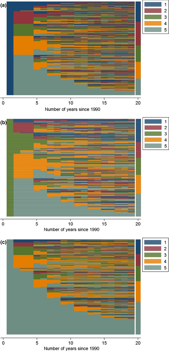
Neighbourhood histories 1990–2008 (10% sample of histories) of those leaving the parental home 1990–1991 by parental neighbourhood quintile (1, 3 and 5). (a) Parental neighbourhood quintile 1 in 1990 (low poverty neighbourhood). (b) Parental neighbourhood quintile 3 in 1990. (c) Parental neighbourhood quintile 5 in 1990 (poverty concentration neighbourhood) Source: Authors’ calculations on GeoSweden dataset
Figure 1(b) shows the neighbourhood histories of those whose parents lived in quintile 3 neighbourhoods (the middle category, represented by the green colour). Figure 1(b) shows a pattern that is roughly comparable with that in Figure 1(a), although those starting in quintile 3 are slightly more likely to move to quintile 3 and 4 neighbourhoods immediately after leaving the parental home. It is striking that those who started in quintiles 1 and 3 have very similar outcomes after 18 years (compare the final columns of Figures 1(a) and (b)). After 18 years there is a roughly equal distribution over the 5 neighbourhood types, regardless of where people started.
Figure 1(c) shows a radically different picture. These are the histories of those whose parents lived in quintile 5 (high poverty concentration) neighbourhoods in 1990 (represented by the colour grey). Table III has already shown that these people are much more likely than others to be exposed to poverty concentration neighbourhoods over their life course. Two thirds of the home leavers with parents in a high poverty concentration neighbourhood move to a similar neighbourhood when they leave the parental home. Over the years, many subsequently move to more affluent neighbourhoods. Nevertheless, the final column in Figure 1(c) shows that after 18 years they are much more likely than others to live in a poverty concentration neighbourhood themselves. It is important to note that the neighbourhood careers of those starting in high poverty concentration neighbourhoods are very diverse. Many histories show episodes in quintile 1 and 2 neighbourhoods (represented by the colours blue and red), but not as many as in Figure 1(a) with the histories of those starting off in low poverty neighbourhoods. Although there is clear evidence of intergenerational transmission of neighbourhood poverty in Figure 1(a)–(c), the neighbourhood careers of individuals starting in similar types of neighbourhoods are also highly heterogeneous in the short term.
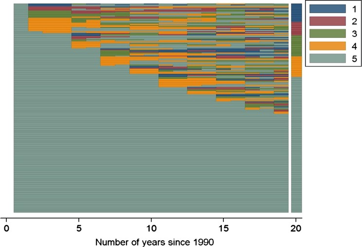
Figure 2 shows the neighbourhood histories of ethnic minority children who lived with their parents in a poverty concentration neighbourhood (quintile 5) in 1990. The difference with the full population (Figure 1(c)) is striking. Ethnic minorities are much more likely than the general population (the majority of whom are Swedish-born) to move into high poverty concentration neighbourhood in the year they leave the parental home. They are also much more likely to spend a considerable amount of time in poverty concentration neighbourhoods during their neighbourhood histories. However, perhaps the most striking difference between Figures 1(c) and 2 is the difference in the final destinations of the ethnic minorities compared with the general population. Individuals from ethnic minorities with parents in a high poverty concentration neighbourhood are much more likely than others (roughly two thirds compared with about one third) to end up in a similar type neighbourhood after 18 years. The figures demonstrate that neighbourhood disadvantage is transmitted particularly strongly between generations of ethnic minority families. It is important to keep in mind that the ‘choice’ to live in low-income neighbourhoods may also be a positive one, based on social networks or proximity to specific facilities (Manley and van Ham 2011).
Figure 2.
Neighbourhood histories 1990–2008, ethnic minorities (no sample but full population) with parental neighbourhood quintile 5 in 1990Source: Authors’ calculations on GeoSweden dataset
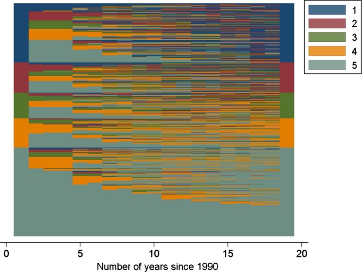
Figures 1 and 2 contain selections of neighbourhood histories based on the parental neighbourhood in 1990. There are many other ways in which the neighbourhood histories can be ordered and categorised. One such alternative categorisation is based on whether people show downward or upward mobility over the period 1990–2008, or whether they experience a stable history over this timeframe. As an illustration, we show the stable mobility histories in Figure 3. In this figure all five parental neighbourhood quintiles are represented on the left hand side. Each of the histories starts with the same colour it ends with (the same neighbourhood quintile) and hence we labelled these stable neighbourhood histories. A major advantage of our visualisation method is that it reveals that although the histories are stable in terms of starting and end points, there is a lot of mobility in between. The colour coding clearly shows that the stable quintile 1 histories show many more episodes in quintile 1 and 2 (blue and red) than the other histories. On the other hand, the stable quintile 5 (high poverty concentration neighbourhoods) histories contain many more episodes in quintile 4 and 5 neighbourhoods. These results show great continuity in neighbourhood status over the life course.
Multivariate models
To understand how neighbourhood histories have developed over time, we modelled neighbourhood outcomes at 5, 12 and 18 years after leaving the parental home using ordered logit regression (Table IV). This enables us to investigate whether the intergenerational transmission of neighbourhood status visible in the figures remains important after controlling for other attained, inherited or ascribed individual characteristics. Informed by the above visualisations, we have included the parental neighbourhood quintile in 1990 and a dummy variable to indicate ethnicity. To see if the intergenerational transmission of neighbourhood poverty is mediated by ethnicity, we included an interaction effect between ethnicity and parental neighbourhood type. For each of the years we show a model with and without parental income in 1990 because we want to know whether neighbourhood outcomes for children are a result of parental income or parental neighbourhood. Since we know from the literature on the intergenerational transmission of disadvantage that the income of parents and children is related, it is likely that any similarity in neighbourhood is simply a result of income. Although this would be an interesting finding in itself, here we are looking for an independent effect of the parental neighbourhood on the neighbourhood outcomes of children.
The results clearly show that the parental neighbourhood is a strong predictor of neighbourhood (dis)-advantage for children 5, 12 and 18 years after leaving the parental home. The higher the poverty concentration of the parental neighbourhood, the higher the poverty concentration of the neighbourhood of their children later in life. It is important to note that this effect holds after controlling for a range of individual and household characteristics, including parental income. The effect of being a non-Western immigrant on neighbourhood outcomes is more complicated. The main effect for non-Western immigrants is not significant in the models unless parental income is also included. The only significant effect can be found in the model with parental income at 5 years after leaving the parental home. Here, non-Western immigrants are much more likely to live in a poverty concentration neighbourhood than others. This indicates that non-Western immigrants are disadvantaged in the first years after leaving the parental home, but then catch up later in life. The interaction effect between immigrant status and parental neighbourhood is only significant after 12 and 18 years for those with parents in the highest poverty concentration neighbourhoods. However, the effects disappear when controlled for parental income. This leads to the broad conclusion that the ethnicity effect found in the visual analysis of neighbourhood histories is caused by income differences between groups.
The control variables show that there are no significant gender or child effects on neighbourhood outcomes. Those living with a partner are less likely to end up in poverty concentration neighbourhoods than singles. This is most likely due to the higher level of resources available to households with two earners. After 5 years, those with a middle level of education are the least likely to end up in poverty concentration neighbourhoods compared with those with lower and university-level education. For those with a university-level education, this can be explained by the fact that they start their housing career somewhat later due to investments in their human capital. This is confirmed by the finding that after 18 years those with a university degree are the least likely to end up in a poverty concentration neighbourhood. Greater levels of income from work reduce the probability of ending up in a poverty concentration neighbourhood, while being on social benefits increases the probability. Those living in public rented accommodation are the most likely to end up in poverty concentration neighbourhoods, followed by those in private renting, cooperative housing and owner-occupied housing.
The final models in Table V report the effect of cumulative exposure to high poverty concentration neighbourhoods (quintile 5) over the full 18-year period after leaving the parental home. The maximum exposure time in this model is therefore 18 years. The results clearly demonstrate that individuals who lived with their parents in quintile 4 and especially quintile 5 neighbourhoods in 1990 spend significantly longer in poverty concentration neighbourhoods over the next 18 years than those who grew up in the low poverty concentration neighbourhoods. Non-Western immigrants have especially long exposure times to high poverty concentration neighbourhoods, even after controlling for parental income. The interaction effects between immigrant status and parental neighbourhood do not indicate an additional effect for immigrants (which was the case in a model without parental income, effects not shown). The control variables show that having a middle-level income reduces the cumulative exposure to poverty concentration neighbourhoods. Having a high mean income and an increase in income during the 18 years (measured by income range) also reduce cumulative exposure to poverty neighbourhoods. In contrast, receiving social benefits increases exposure to poverty concentration neighbourhoods. With increasing number of years in public renting, the exposure to poverty concentration neighbourhoods increases, while spending greater periods of time in home ownership reduces the exposure to the most disadvantaged neighbourhoods.
Conclusions
This is the first study to construct and visualise the entire neighbourhood histories of a large group of individuals over a long period of time. We investigated the intergenerational transmission of neighbourhood poverty in Stockholm through the effect of the parental neighbourhood on individual neighbourhood histories over a period of almost two decades. By constructing neighbourhood histories, this study has sought to empirically operationalise the concept of unique individual biographies emphasised by life course theory (Dykstra and van Wissen 1999). We argued that accurately measuring the extent to which parental neighbourhood context is transmitted to children and understanding the factors that lead to neighbourhood sorting by individuals is critical to understanding residential outcomes later in life. There is a vast literature on neighbourhood effects that ties individual outcomes to the neighbourhood in which they currently live. By taking a much longer term view we have demonstrated that individual outcomes are influenced over a much longer timescale: where individuals lived up to 18 years ago is important for their current outcomes.
Using innovative visualisation techniques, we have shown that individuals sort themselves into neighbourhoods across the income spectrum as they move through the life course. This sorting process is the result of individual preferences, resources, but also opportunities and constraints offered by the housing market. The graphs clearly showed that although many individuals experienced an initial drop in neighbourhood status immediately after leaving the parental home, many catch up in their subsequent residential career. However, we also demonstrated that children living with their parents in high poverty concentration neighbourhoods are very likely to end up in similar neighbourhoods much later in life when they are adults, especially when they are an ethnic minority. These results were confirmed by the multivariate analyses. The results show that the intergenerational transmission of disadvantage is a powerful mechanism explaining the residential outcomes of individuals across their life course. It is important to note that we found these results for Sweden, one of the Nordic countries more commonly associated with equality in outcomes. Based on our results we would expect to find even stronger intergenerational transmission of disadvantage in a country like the UK, which has a more segmented housing market and a more unequal income distribution than Sweden. The study has also shown that the parental neighbourhood is highly predictive for the cumulative exposure to poverty concentration neighbourhoods over the life course. Those individuals who lived with their parents in high poverty concentration neighbourhoods spend significantly longer in such neighbourhoods over the next 18 years than those who grew up in low poverty concentration neighbourhoods. Ethnic minorities were found to have the longest cumulative exposure to poverty concentration neighbourhoods.
That parental neighbourhood type has such a long-lasting impact on exposure, even after controlling for a variety of changes occurring elsewhere in the life course, suggests that disadvantage is not solely transmitted through parental income, but is also linked to living in poverty neighbourhoods. Based on our data we cannot identify the causal mechanisms underlying the intergenerational transmission of neighbourhood poverty. There are several possible explanations for the effects found. One such explanation is that children choose to live in neighbourhood types that are familiar from their childhood. Another possible explanation could be that children choose to live in close proximity to their parents, and therefore end up in similar neighbourhoods, or choose to live in a neighbourhood with similar (ethnic group) specific services. The effects might also be the result of a lack of choice due to the structure and institutional arrangements of the housing market. A more complex set of explanations might be derived from the neighbourhood effects literature. Socialisation and peer group effects, and a lack of positive role models (see Galster 2012), might lead those growing up in high poverty concentration neighbourhoods to develop deviating labour market attitudes and values, and might lead to a lack of informal skills needed on the labour market. Although we control for individual income in our models, income might not be a sufficient proxy for these factors which in turn might affect the choice (or lack of choice) to live in a poverty concentration neighbourhood as adults. Future research can shed more light on these possible underlying mechanisms.
This study has showcased the contribution that geography as an academic discipline can make to the discussion on intergenerational mobility. Where sociologists focus mainly on intergenerational mobility across class and occupations, and economists typically analyse income and earnings mobility (D'Addio 2007; Solon 1999), our study has demonstrated the importance of the spatial dimension of intergenerational transmission of (dis)advantage. The results of our study also have wider implications for other areas of geographical study. The literature on neighbourhood effects typically uses simple point-in-time measures of neighbourhood. We have demonstrated that it is important to measure neighbourhood experiences over longer periods of time because for some groups disadvantage is both inherited and highly persistent, while for other groups living in poverty neighbourhoods is only a temporary state. We have clearly demonstrated that adult exposure to poverty concentration neighbourhoods is linked to the neighbourhood that an individual lived in with their parents. This indicates that neighbourhood effects might run between generations and suggests that not just the current neighbourhood, but the whole neighbourhood history, should be taken into account when investigating whether people are disadvantaged by where they live. The results also have wider implications for the study of segregation. Understanding why people live in certain types of neighbourhoods cannot be simply understood from their current characteristics, but a full understanding should take into account the neighbourhood biographies of individuals. Finally, this study has demonstrated the value of visualisation techniques for spatial and temporal data. Visualising neighbourhood histories allowed us to contextualise events and transitions within a true life course framework.
Acknowledgments
The research reported in this paper was made possible through the financial support of the Institute for Housing and Urban Research (IBF) at Uppsala University, Sweden and the financial support of the EU (NBHCHOICE Career Integration Grant under FP7-PEOPLE-2011-CIG). We would like to thank the editor and the anonymous reviewers for their comments.
Notes
The Stockholm metropolitan region includes the municipalities of Stockholm and Solna, along with those municipalities of the Stockholm labour market region where the majority of the commuting flow is into either Stockholm or Solna.
The calculations stop when the number of neighbours exceeds 500. Since the software uses a 100 by 100 metre grid, the total number of neighbours included is often slightly higher than 500.
Income from work is calculated as the sum of: salary payments, income from active businesses and tax-based benefits that employees accrue as terms of their employment (including sick or parental leave, work-related injury or illness compensation, daily payments for temporary military service or giving assistance to a disabled relative).
The figures and tables that follow are presented as near as possible to the primary discussion of the relevant information, rather than necessarily in the order in which they are first mentioned.
The reason for modelling outcomes after 5 (in 1995) instead of the more logical 6 years is that data on tenure only is available in 1990, 1995, 2000, 2002, 2004, 2006 and 2008. We have roughly estimated tenure for intervening years.
References
- Aisenbrey S, Fasang AE. New life for old ideas: the ‘second wave’ of sequence analysis bringing the ‘course’ back into the life course. Sociological Methods and Research. 2010;38:420–62. [Google Scholar]
- Becker GS, Tomes N. An equilibrium theory of the distribution of income and intergenerational mobility. Journal of Political Economy. 1979;87:1153–89. [Google Scholar]
- Bisin A, Verdier T. On the cultural transmission of preferences for social status. Journal of Public Economics. 1998;70:75–97. [Google Scholar]
- Blaauboer M. The impact of childhood experiences and family members outside the household on residential environment choices. Urban Studies. 2011;48:1635–50. doi: 10.1177/0042098010377473. [DOI] [PubMed] [Google Scholar]
- Brzinsky-Fay C, Kohler U, Luniak M. Sequence analysis with Stata. The Stata Journal. 2006;6:435–60. [Google Scholar]
- Cabinet Office. Opening doors, breaking barriers: a strategy for social mobility. London: Cabinet Office; 2011. [Google Scholar]
- Clark WAV, Withers SD. Family migration and mobility sequences in the United States: spatial mobility in the context of the life course. Demographic Research. 2007;17:591–622. [Google Scholar]
- Clark WAV, Dieleman FM. Households and housing: choice and outcomes in the housing market. New Brunswick NJ: CUPR Press; 1996. [Google Scholar]
- Clark WAV, Huang Y. The life course and residential mobility in British housing markets. Environment and Planning A. 2003;35:323–39. [Google Scholar]
- Clark WAV, Ledwith V. Mobility, housing stress, and neighborhood contexts: evidence from Los Angeles. Environment and Planning A. 2006;38:1077–93. [Google Scholar]
- Clark WAV, Deurloo M, Dieleman FM. Housing careers in the United States, 1968–93: modelling the sequencing of housing states. Urban Studies. 2003;40:143–60. [Google Scholar]
- Coulter R, van Ham M. Following people through time: an analysis of individual residential mobility biographies. Housing Studies. forthcoming. [Google Scholar]
- Crowder K, South SJ. Race, class, and changing patterns of migration between poor and nonpoor neighborhoods. American Journal of Sociology. 2005;110:1715–63. [Google Scholar]
- D'Addio AC. Intergenerational transmission of disadvantage: mobility or immobility across generations. Paris: OECD Social, Employment and Migration Working Papers No. 52 OECD Publishing; 2007. [Google Scholar]
- Duncan GJ, Raudenbush SW. Neighborhoods and adolescent development: how can we determine the links? In: Booth A, Crouter AC, editors. Does it take a village? Community effects on children, adolescents, and families. Mahwah NJ: Lawrence Erlbaum; 2001. pp. 105–36. [Google Scholar]
- Durlauf SN. Neighbourhood effects. In: Henderson JV, Thisse JF, editors. Handbook of regional and urban economics. Volume 4: Cities and geography. Amsterdam: Elsevier; 2004. pp. 2173–242. [Google Scholar]
- Dykstra P, van Wissen L. Introduction: the life course approach as an interdisciplinary framework for population studies. In: van Wissen L, Dykstra P, editors. Population issues: an interdisciplinary focus. New York: Plenum Press; 1999. pp. 1–22. [Google Scholar]
- Elder GH. Time, human agency, and social change: perspectives on the life course. Social Psychology Quarterly. 1994;57:4–15. [Google Scholar]
- Ellen IG, Turner MA. Does neighbourhood matter? Assessing recent evidence. Housing Policy Debate. 1997;8:833–66. [Google Scholar]
- Esping-Andersen G. The three worlds of welfare capitalism. Princeton NJ: Princeton University Press; 1990. [Google Scholar]
- Feijten P. Life events and the housing career: a retrospective analysis of timed effects. Delft: Eburon; 2005. [Google Scholar]
- Feijten P, Mulder CH. Life course experience and housing quality. Housing Studies. 2005;20:571–88. [Google Scholar]
- Feijten P, Hooimeijer P, Mulder CH. Residential experience and residential environment choice over the life-course. Urban Studies. 2008;45:141–62. [Google Scholar]
- Galster G. An economic efficiency analysis of deconcentrating poverty populations. Journal of Housing Economics. 2002;11:303–29. [Google Scholar]
- Galster G. The mechanism(s) of neighbourhood effects: theory, evidence, and policy implications. In: van Ham M, Manley D, Simpson L, Bailey N, Maclennan D, editors. Neighbourhood effect research: new perspectives. Dordrecht: Springer; 2012. pp. 23–56. [Google Scholar]
- Geist C, McManus PA. Geographical mobility over the life course: motivations and implications. Population, Space and Place. 2008;14:283–303. [Google Scholar]
- Hedin K, Clark E, Lundholm E, Malmberg G. Neoliberalization of housing in Sweden: gentrification, filtering, and social polarization. Annals of the Association of American Geographers. 2012;102:443–63. [Google Scholar]
- Helderman A, Mulder CH. Intergenerational transmission of homeownership: the roles of gifts and continuities in housing market characteristics. Urban Studies. 2007;44:231–47. [Google Scholar]
- Henretta JC. Parental status and child's home ownership. American Sociological Review. 1984;49:131–40. [Google Scholar]
- Jencks C, Mayer SE. The social consequences of growing up in a poor neighborhood. In: Lynn LE, McGeary MGH, editors. Inner-city poverty in the United States. Washington DC: National Academy Press; 1990. pp. 111–86. [Google Scholar]
- Kasarda JD. Jobs, migration, and emerging urban mismatches. In: McGeary MGH, Lynn LE, editors. Urban change and poverty. Washington DC: National Academy Press; 1988. pp. 148–98. [Google Scholar]
- Kim TK, Horner MW, Marans RW. Life cycle and environmental factors in selecting residential and job locations. Housing Studies. 2005;20:457–73. [Google Scholar]
- Kuntz J, Page ME, Solon G. Are point-in-time measures of neighborhood characteristics useful proxies for children's long-run neighborhood environment? Economic Letters. 2003;79:231–7. [Google Scholar]
- Kurz K. Labour market position, intergenerational transfers and home-ownership. A longitudinal analysis for West German birth cohorts. European Sociological Review. 2004;20:141–59. [Google Scholar]
- Maloutas T. Introduction: residential segregation in context. In: Maloutas T, Fujita K, editors. Residential segregation in comparative perspective. Making sense of contextual diversity. Farnham: Ashgate; 2012. pp. 1–36. [Google Scholar]
- Manley DJ, van Ham M. Choice-based letting, ethnicity and segregation in. England Urban Studies. 2011;48:3125–43. [Google Scholar]
- Manley DJ, van Ham M. Neighbourhood effects, housing tenure, and individual employment outcomes. In: van Ham M, Manley D, Bailey N, Simpson L, Maclennan D, editors. neighbourhood effects research: new perspectives. Berlin: Springer; 2012. pp. 147–74. [Google Scholar]
- Massey DS, Gross AB, Shibuya K. Migration, segregation, and the concentration of poverty. American Sociological Review. 1994;59:425–45. [Google Scholar]
- Meen G, Meen J, Nygaard C. A tale of two Victorian cities in the 21st century. ICHUE – Discussion papers. 2007 No. 007. [Google Scholar]
- Menard S. Applied logistic regression analysis. London: Sage; 2002. [Google Scholar]
- Mulder CH, Hooimeijer P. Residential relocations in the life course. In: van Wissen L, Dykstra P, editors. Population issues: an interdisciplinary focus. New York: Plenum Press; 1999. pp. 159–86. [Google Scholar]
- Mulder CH, Smits J. First-time home-ownership of couples. The effect of inter-generational transmission. European Sociological Review. 1998;15:323–37. [Google Scholar]
- OECD. Economic policy reforms 2010: going for growth. Paris: Organization for Economic Cooperation and Development; 2010. [Google Scholar]
- Östh J, Malmberg B, Andersson E. Analysing segregation using individualized neighbourhoods. In: Lloyd CD, Shuttleworth I, Wong D, editors. Social-spatial segregation: concepts, processes and outcomes. Bristol: Policy Press; forthcoming. [Google Scholar]
- Pollock G. Holistic trajectories: a study of combined employment, housing and family careers by using multiple-sequence analysis. Journal of the Royal Statistical Society: Series A. 2007;170:167–83. [Google Scholar]
- Quillian L. How long are exposures to poor neighborhoods? The long-term dynamics of entry and exit from poor neighbourhoods. Population Research and Policy Review. 2003;22:221–49. [Google Scholar]
- Rabe B, Taylor M. Residential mobility, quality of neighbourhood and life course events. Journal of the Royal Statistical Society: Series A. 2010;173:531–55. [Google Scholar]
- Rossi PH. Why families move. A study in the social psychology of urban residential mobility. Glencoe IL: Free Press; 1980. [Google Scholar]
- Sampson RJ, Wilson WJ. Toward a theory of race, crime, and urban inequality. In: Hagan J, Peterson RD, editors. Crime and Inequality. Stanford, CA: Stanford University Press; 1995. pp. 177–90. [Google Scholar]
- Simpson L, Finney N. Spatial patterns of internal migration: evidence for ethnic groups in Britain. Population, Space and Place. 2009;15:37–56. [Google Scholar]
- Solon G. Intergenerational mobility in the labor market. In: Ashenfelter O, Layard R, Card D, editors. Handbook of labor economics volume 3. Dordrecht: Elsevier; 1999. pp. 1761–800. [Google Scholar]
- South SJ, Crowder KD. Escaping distressed neighborhoods: individual, community, and metropolitan influences. American Journal of Sociology. 1997;102:1040–84. [Google Scholar]
- South SJ, Deane GD. Race and residential mobility: individual determinants and structural constraints. Social Forces. 1993;72:147–67. [Google Scholar]
- Stovel K, Bolan M. Residential trajectories: using optimal alignment to reveal the structure of residential mobility. Sociological Methods and Research. 2004;32:559–98. [Google Scholar]
- van Ham M. Housing behaviour. In: Clapham D, Clark WAV, Gibb K, editors. Handbook of housing studies. London: Sage; 2012. chapter 3. [Google Scholar]
- van Ham M, Manley D. Social housing allocation, choice and neighbourhood ethnic mix in England. Journal of Housing and the Built Environment. 2009;24:407–22. [Google Scholar]
- van Ham M, Manley D. The effect of neighbourhood housing tenure mix on labour market outcomes: a longitudinal investigation of neighbourhood effects. Journal of Economic Geography. 2010;10:257–82. [Google Scholar]
- van Ham M, Manley D, Bailey N, Simpson L, Maclennan D. Neighbourhood effects research: new perspectives. Dordrecht: Springer; 2012. [Google Scholar]
- Vartanian TP, Buck PW, Gleason P. Intergenerational neighborhood-type mobility: examining differences between blacks and whites. Housing Studies. 2007;22:833–56. [Google Scholar]
- Wilson WJ. The truly disadvantaged. Chicago IL: University of Chicago Press; 1987. [Google Scholar]