

Abstract
A minimum mathematical model of the marine pelagic microbial food web has previously shown to be able to reproduce central aspects of observed system response to different bottom-up manipulations in a mesocosm experiment Microbial Ecosystem Dynamics (MEDEA) in Danish waters. In this study, we apply this model to two mesocosm experiments (Polar Aquatic Microbial Ecology (PAME)-I and PAME-II) conducted at the Arctic location Kongsfjorden, Svalbard. The different responses of the microbial community to similar nutrient manipulation in the three mesocosm experiments may be described as diatom-dominated (MEDEA), bacteria-dominated (PAME-I), and flagellated-dominated (PAME-II). When allowing ciliates to be able to feed on small diatoms, the model describing the diatom-dominated MEDEA experiment give a bacteria-dominated response as observed in PAME I in which the diatom community comprised almost exclusively small-sized cells. Introducing a high initial mesozooplankton stock as observed in PAME-II, the model gives a flagellate-dominated response in accordance with the observed response also of this experiment. The ability of the model originally developed for temperate waters to reproduce population dynamics in a 10°C colder Arctic fjord, does not support the existence of important shifts in population balances over this temperature range. Rather, it suggests a quite resilient microbial food web when adapted to in situ temperature. The sensitivity of the model response to its mesozooplankton component suggests, however, that the seasonal vertical migration of Arctic copepods may be a strong forcing factor on Arctic microbial food webs.
In the marine pelagic, the photic zone microbial food web functions as the interface between the nutrient and carbon chemistry of the ocean on one side, and the food chain transferring primary production to harvestable resources or exporting it to the ocean's interior on the other. The complexity of the system is often emphasized, in particular when considering the genetic diversity within each of the functional groups comprising the microbial part of the pelagic food web. Deep diversity within each functional group, does, however not necessarily mean that the trophic network connecting these functional groups cannot be represented by a relatively small set of dominating pathways. How small such a set is, and whether there exists a minimum model that has enough, but not more, variables and interactions to capture the dominating dynamic features of the system, can only be answered by challenging the explanatory power of such a model with experimental and/or observational data. Here, we combine mesocosm experiments and modeling to find such a minimum set to reveal basic properties of marine ecosystem functioning.
Many contemporary modeling efforts aim at representing the microbial food web in global circulation models. With a primary goal to reproduce global datasets like e.g., satellite-observed chlorophyll this effort has been particularly intensive for its phytoplankton part (e.g., Le Quere et al. 2005; Follows et al. 2007). There are also models analyzing steady state relationships between bottom-up and top-down forces in the microbial food web and the relationship to fish production (e.g., Stock et al. 2008). Here, we focus on the response of this system at much smaller time- and space-scales using nutrient-perturbed mesocosms.
Dissolved mineral nutrients can enter the microbial food web through phytoplankton in different size-classes as well as through heterotrophic prokaryotes (henceforth termed bacteria). The microbial organisms using dissolved nutrients (henceforth termed osmotrophs) thus span about three orders of magnitude in linear size, equivalent to about nine orders of magnitude in volume. Whether the nutrients enter through autotrophic flagellates, diatoms, or bacteria will have consequences, not only for the size-structure of the food web, but also for its autotroph–heterotroph balance. A simple hypothesis could be that the position of the dominating entry-point is determined by the relative competitive abilities between osmotrophs. Competitive ability has received a lot of attention in classical phytoplankton ecology (e.g., Harris 1980; Tilman et al. 1982; Sommer 1985) where the organism's requirement, capacity for rapid uptake, rapid growth, and storage, all play roles that differ depending on the concentration level and temporal variability of the limiting nutrient. At permanently low nutrient concentrations, it is often argued that small organisms with their high surface-to-volume ratio are the superior competitors (e.g., Aksnes and Cao 2011). Following this argument, a simple hypothesis would be that an addition of easily degradable organic material such as glucose should force the entry point for the mineral nutrients toward heterotrophic bacteria. How large diatoms could dominate in situations with nutrient competition may, however, seem difficult to explain without a more complex model.
It is known that the population response in the osmotroph community can be strongly modified by the structure of the predator community as demonstrated experimentally (e.g., Stibor et al. 2004; Vadstein et al. 2012), and summarized in the concept of “loopholes” (Irigoien et al. 2005). Using simple gnotobiotic model systems in chemostats, it has also been shown how a selective grazing pressure on bacteria in the presence of an inferior diatom competitor for phosphate, can give a diatom-dominated system with few bacteria and a very limited capacity for glucose consumption (Pengerud et al. 1987). This effect was later reproduced under the near-natural conditions of a mesocosm experiment where Havskum et al. (2003) demonstrated how the combined addition of silicate and glucose led to a bloom of large chain-forming diatoms and a reduction in the system's ability to consume the added glucose (subsequently referred to as the MEDEA experiment). An experiment in the Arctic (PAME-I) with similar bottom-up manipulations gave, however, the opposite effect, i.e., when silicate addition was combined with glucose, the result was a discontinuation of a rising diatom bloom (Thingstad et al. 2008). With nitrate and ammonium used as nitrogen source in the MEDEA and PAME-I experiments, respectively, we hypothesized that this difference in N-source could have influenced the size-structure of the diatom community as suggested by Stolte and Riegman (1995). In a subsequent experiment in the same Arctic location (PAME-II), an ammonium vs. nitrate treatment was, therefore, incluced in the factorial design. As we show here, this experiment resulted in a flagellate-dominated phytoplankton bloom and gave no clear signs of the effects expected from the other treatments (glucose, silicate, and NH4/NO3).
At first sight, the minimum food web model (Fig. 1) successfully used to describe central features of the response seen in the MEDEA-experiment (Thingstad et al. 2007), may therefore seem representative only of the single case of one mesocosm experiment. Qualitatively, however, one can argue that only minor modifications may be required for this structure also to provide explanations for both of the two PAME experiments (Thingstad and Cuevas 2010).
Figure 1.
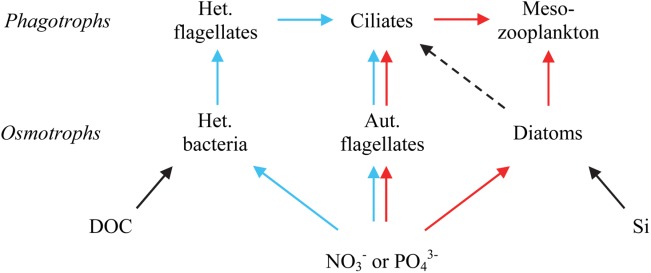
The microbial food web model formulated mathematically by Thingstad et. al (2007), amended with the assumption (dashed line) used for the PAME-I experiment that ciliates graze on small diatoms. The model contains three alternative entrances for dissolved mineral nutrients: heterotrophic (Het.) bacteria, autotrophic (Aut.) flagellates, and diatoms and can graphically be described as consisting of a right (red) and a left (blue) pentagon. Remineralization pathways omitted for clarity.
In this article, we present data from the PAME experiments and demonstrate the ability of the previously published model to reproduce the observed response patterns, making as few modifications as possible to the original model. By summarizing three contrasting responses, the extended model serves as an important step toward a more generalized understanding of microbial food web dynamics. At the same time, however, it emphasizes how relatively small differences in initial food web composition may alter system responses and therefore also serves as a warning against firm predictive statements. Efforts in demonstrating reproducibility between experiments may, therefore, seem at least as important as efforts in replication within mesocosm experiments.
Materials and methods
Mesocosm setup and sampling procedures
The two mesocosm experiments were conducted in Kings Bay, Northern Spitsbergen (78°55′N, 11°56′E) from 02 August to 15 August 2007 (PAME-I) and from 28 June to 10 July 2008 (PAME-II) as part of the International Polar Year (http://ipy.no/). High-density translucent polyethylene tanks of 1 m3 (Ecobulk MX-HV 1000; Schütz®, Selters, Germany) were used as experimental units. They were uniformly filled with fjord water from the outer (PAME-I) or middle (PAME-II) of the fjord, avoiding a nearby sediment-containing riverine inflow. To ensure sampling from within a homogenous water-body, a layer with minimal gradients in temperature, salinity, and fluorescence was located using a Conductivity Temperature Density (CTD) (Saiv Instruments). Based on this, the tanks were filled with water from between 5.0 m and 6.0 m depth to a volume of 700 (PAME-I) liter and 900 (PAME-II) liter, using a submersible centrifugal pump with no metal parts in contact with the water-flow. The salinity was 32.7 psu in 2007 (PAME-I) and 34.4 psu in 2008 (PAME-II). For the experimental period, the tanks were anchored in the harbor of Ny Ålesund Research Station. Temperature in the tanks varied with surface water temperature, and ranged from 4.7°C to 7.5°C during PAME-I and 3.8°C to 7.5°C during PAME-II.
To create the experimental setup illustrated in Fig. 2, nutrients were added from concentrated aqueous stocks to nominal final concentrations (calculated assuming 700 L and 900 L constant volume for PAME-I and PAME-II, respectively) as shown in Table1. The tanks were mixed using a manual paddle before each sampling and after nutrient additions. In addition, tanks were gently mixed by the natural wave action in the harbor. Samples from the tanks were collected in polyethylene carboys using silicon tubing and gentle suction, and brought to nearby laboratories in Ny Ålesund for immediate analysis. Samples were collected daily between 07:00 h and 08:00 h, prior to nutrient addition.
Figure 2.
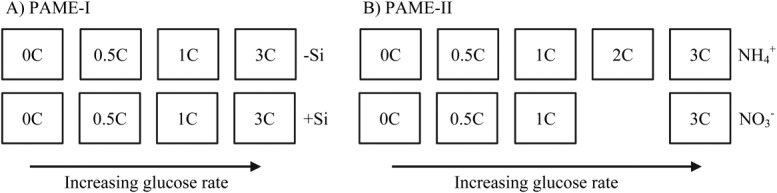
Experimental setup with eight (PAME-I) and nine (PAME-II) tanks, all receiving the same dose of N and P in Redfield ratio (C : N : P = 106 : 16 : 1 molar) arranged in two 4-point glucose-addition gradients (0, 0.5, 1, 3 × Redfield in glucose-C; PAME-I) or one 4- and one 5-point glucose-addition gradient (0, 0.5, 1, (2), 3 × Redfield in glucose-C; PAME II). (A) In PAME-I one gradient (−Si) received no experimental addition of silicate, the other (+Si) was kept silicate replete. (B) In PAME-II one gradient ( ) received N as NH4Cl and one gradient (
 ) as NaNO3. All tanks were kept silicate replete.
Table 1.
Initial nutrient values and daily additions of carbon (glucose), phosphate, and nitrate in the experiments. Silicate was added on day 4, 5, and 9 in PAME I and on day 0–4 and 10 in PAME II. The values for daily additions are final nominal concentrations..
| Experiment | Tank label | Glucose level | d-glucose | KH2PO4 | NH4Cl or NaNO3† | Na2SiO3‡ |
|---|---|---|---|---|---|---|
| μmol C L−1 | nmol P L−1 | μmol N L−1 | μmol Si L−1 | |||
| PAME-I | Initial values* | 77§ | 80 | 0.13¶ | 1.31 | |
| 0C | 0 | 0 | 143 | 2.29 | 8.6/17.1/25.7 | |
| 0.5C | 0.5 | 7.6 | 143 | 2.29 | 8.6/17.1/12.9 | |
| 1C | 1 | 15.1 | 143 | 2.29 | 8.6/17.1/ 0 | |
| 3C | 3 | 45.4 | 143 | 2.29 | 8.6/17.1/ 0 | |
| PAME-II | Initial values* | 95§ | 70 | 0.08¶ | 1.23 | |
| 0C | 0 | 0 | 100 | 1.6 | 1.5/4.5/1.5/1.5/1.5/3.0 | |
| 0.5C | 0.5∥ | 5.25 | 100 | 1.6 | 1.5/4.5/1.5/1.5/1.5/3.0 | |
| 1C | 1 | 10.5# | 100 | 1.6 | 1.5/4.5/1.5/1.5/1.5/3.0 | |
| 2C | 2 | 21.0 | 100 | 1.6 | 1.5/4.5/1.5/1.5/1.5/3.0 | |
| 3C | 3 | 31.5 | 100 | 1.6 | 1.5/4.5/1.5/1.5/1.5/3.0 |
Initial nutrient values were measured as follows: dissolved phosphate, silicate, and ammonium were measured immediately after sampling according the methods described in Koroleff (1983), Valderrama (1995), and Holmes et al. (1999), respectively. Nitrite and nitrate were measured by autoanalyzer after the experiments using samples preserved with chloroform and stored refrigerated. Total organic carbon (TOC) was measured using high temperature catalytic oxidation as described in Børsheim (2000).
In PAME-I, nitrogen was added as NH4Cl. In PAME-II, nitrogen was added as NaNO3 in the gradient and as NH4Cl in the NH4-gradient.
In PAME-I, silicate was added to the +Si units in only. Na2SiO3 was added as an aqueous solution with pH adjusted to 7.5 with HCl.
Total organic carbon (TOC)
Ammonia + nitrate + nitrite
Glucose level 0.5 only in the NH4-gradient.
By mistake, 1C in the NH4-gradient received double amount of glucose (3.5 μmol C) on day 5 and consequently no glucose was added on day 6.
Chl a
Chlorophyll a (Chl a) was measured fluorometrically according to Parsons et al. (1984). Total Chl a biomass (filtered onto 47 mm diameter, 0.2 μm pore size nucleopore filters was measured every day and Chl a biomass in size fractions (filtered onto 47 mm diameter nucleopore filters of pore sizes 0.2 μm, 1 μm, 5 μm, and 10 μm) every second day. The filters were extracted in 90% acetone, at 4°C in the dark for 10–12 h, before analyzis on a Turner Designs 10-AU Fluorometer calibrated with pure Chl a (Sigma Chemicals).
Protist and bacteria abundances
Phytoplankton, heterotrophic nanoflagellates (HNF), and bacteria numbers were determined using a FacsCalibur flow cytometer (Becton Dickinson) equipped with an air-cooled laser providing 15 mW at 488 nm with standard filter setup. The phytoplankton counts were obtained from fresh samples with the trigger set on red fluorescence and counted as picophytoplankton, nanophytoplankton I, and nanophytoplankton II based on increasing chlorophyll autofluorescence and side-scatter signal (SSC) signals (Larsen et al. 2001). Samples for enumeration of bacteria and HNF were fixed with glutaraldehyde (0.5% final concentration) and paraformaldehyde (1% final concentration), respectively, stained with SYBR Green I (Molecular Probes, Eugene, Oregon) and analyzed following the recommendations of Marie et al. (1999) for bacteria and Zubkov et al. (2007) for HNF using green fluorescence as trigger. Discrimination of phytoplankton, bacteria, and HNF was based on dot plots of SSC vs. pigment autofluorescence (chlorophyll and phycoerythrin), SSC signal vs. green Deoxyribonucleicacid (DNA)-dye fluorescence, and green DNA-dye fluorescence vs. chlorophyll autofluorescence, respectively.
Ciliates were enumerated using a black and white imaging FlowCAM® II (Fluid Imaging Technologies, Scarborough, Maine, U.S.A.). Samples were analyzed for 30 min using a ×10 objective, in Auto Image mode, and with fluorescence trigger off, to yield a representative size structure of particles ranging from 7 μm to 1000 μm Equivalent Spherical Diameter (ESD) (Alvarez et al. 2011). Ciliates were sorted manually by visual inspection of the image database. In PAME-I, the samples were fixed with pseudolugol (Verity et al. 2007), whereas in PAME-II the samples were analyzed fresh and unpreserved.
Mesozooplankton biomass
Mesozooplankton were sampled at the start of each experiment by filtering 1 m3 of water although a 90 μm WP plankton net in triplicate before, between, and after filling of the meoscosms, and at the end of the experiment by emptying each mesocosm through the same net. Mesozooplankton were fixed immediately in 4% buffered formaldehyde and later identified, enumerated, and sized using a dissecting microscope. Mesozooplankton abundance was converted into carbon biomass by applying size-specific carbon conversion factors as previously described in Nejstgaard et al. (2006).
Grazing
Microzooplankton community grazing impact on the bacteria and phytoplankton communities was quantified by a dilution assay, with quadruplicates of undiluted whole water and highly dilute (10% whole water) treatments, respectively, according to the general approach described by Landry (1993). The diluted and undiluted samples were transferred to dialysis bags and incubated for 24–44 h. The dialysis bags (type Visking 36/32, http://Visking.com) were clear, had a high molecular weight cut off (6–8 kDa), a large surface to volume ratio (ca., 11 cm2 per mL content) and were moving freely inside the mesocosms due to the wave action. This ensured that the content of the dialysis bags were incubated at in situ light and nutrient conditions (Stibor et al. 2006). Bacterial numbers were determined by flow cytometry as described above. The phytoplankton community was analyzed as size fractionated samples for Chl a, by filtering 200 mL onto series of 10 μm, 5 μm, 1 μm, and 0.22 μm pore size nucleopore filters, and analyzed as described above. Grazing was estimated from the negative slope of apparent prey growth rate vs. dilution factor and the standard error (SE) was estimate from the SE of the slope.
Production and respiration
Gross production (GP) and community respiration (CR) were measured with the light and dark bottle technique (Gaarder and Gran 1927). For each sample, six 40 mL glass bottles (3 dark and 3 light) with glass stoppers were incubated in the sea at the bottom level of the mesocosm tanks. Oxygen concentration was measured before and after 24 h incubation using an optode system (Oxy-mini, World Precision Instruments, Florida, U.S.). CR and net community production were calculated as the average of the oxygen change in dark and light bottles, respectively, and GP calculated as GP = NP − CR (CR given as negative changes in oxygen), assuming respiration to be the same in light and dark bottles.
Mathematical model
The trophic structure in Fig. 1, used to discuss conceptually the carbon to nutrient coupling of the PAME-I experiment (Thingstad et al. 2008) was the same as in the mathematical model used to simulate the MEDEA experiment (Thingstad et al. 2007). The mathematical model runs on phosphorous as the common currency, converted to observed values such as abundance or Chl a using fixed conversion factors. To include the ability of ciliates to graze on small diatoms (Verity and Villareal 1986; Montagnes 1996; Hansen et al. 1997), the model was amended with a potential for ciliates to consume diatoms at a maximum clearance rate calculated as fraction c2 of their maximum clearance rate for autotrophic flagellates. Similarly, copepod clarance rate for the small diatoms was reduced with a factor (1 − c2). The differences in model setup for the three runs used to illustrate each experiment are summarized in Table2. The equations and, importantly, all parameter values were otherwise kept as given in Thingstad et al. (2007). The initial state was also calculated as previously described (Thingstad et al. 2007), by assuming that the microbial part (all phosphorous pools except mesozoplankton) initially was in the steady state given by the amount of phosphorous available to the microbial system (total-P) and the amount of P in the mesozooplankton compartment.
Table 2.
Initial conditions, new parameter, and conversion factors used for the model runs. The full parameter set and conversion factors can be obtained in Table 4 in Thingstad et al. (2007).
| MEDEA | PAME-I | PAME-II | ||
|---|---|---|---|---|
| Initial conditions | ||||
| PT nM-P in microbial part | 220 | 220 | 220 | |
| M nM-P in mesozooplankton | 40 | 35 | 65 | |
| New parameter | ||||
| c2 Ciliate clearance rate for small diatoms as fraction of their clearance rate for autotrophic flagellates. Mesozooplankton clearance rate for diatoms reduced by factor (1−c2) | 0 | 0.55 | 0 | |
| Coversion factors | ||||
| P:Chl a | 47.2 n mol P : μg Chl a | |||
| P:bact | 3.33×10⁻⁸ nmol P : bact | |||
| P:HF | 4 10−4 nmol P : HF | |||
| P:Cil | 1 10−2 nmol P : ciliate | |||
| C:P in MZ | 50 mol : mol | |||
In the original model developed for the MEDEA experiment (Thingstad et al. 2007), primary production could only be fitted to observed 14C-based primary production by assuming that diatom photosynthesis was proportional to diatom P-biomass. To explore the fit of the model to our O2-based measurements of gross production (GP) and CR in PAME-I and PAME-II, we explored two alternatives for converting the model's P-cycle to O2 consumption and production rates; one based primarily on P-uptake rates, the other on P-biomasses.
Alternative I: O2 metabolism based on P-uptake
C-fixation assumed proportional to P-uptake in autotrophic flagellates and in diatoms with Redfield C : P stoichiometry (106 : 1 molar ratio). C-fixation was converted to O2-production assuming a photosynthetic quotient of 1 (molar). In addition to this, a primary production term compensated by an identical phytoplankton respiration was assumed as a fraction (10%) of phytoplankton biomass per day. This gives:
where the μ(S) are specific growth rates (unit: d−1) for autotrophic flagellates (AF) and diatoms (D) as indicated by the subscripts, both as functions of free phosphate concentration (S).
For bacteria, the uptake of P is converted to C-biomass produced assuming C : P = 50 (molar) in bacterial biomass. Bacterial oxygen consumption was calculated assuming a respiration coefficient r = 0.67 and an O2 : C ratio of 1. For the predators, C ingested is calculated by converting P ingested using the C : P ratio in the prey (106 for autotrophs, 50 for heterotrophs). C incorporated is calculated from P-uptake using the model's P-yield (Y) and the the difference between ingested and incorporated C assumed to be respired with an O2 : C-ratio of 1.
This gives:
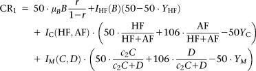 |
where I and Y are the modeled ingestion rates and P-yields for heterotrophic flagellates (HF), ciliates (C), and mesozooplankton (M) as indicated by the subscripts. c2 is a selectivity factor for mesozooplankton predation on ciliates relative to diatoms kept to c2 = 2 as in the original model.
Alternative II: O2-metabolism based on P-biomass
Assuming a primary production equal to 50% of C-biomass per day gives:
Oxygen consumption from heterotrophs was assumed to be 75% of C-biomass per day and the phytoplankton respiration added as in Alternative I:
Experimental data used to challenge the explanatory power of the model
All PAME-II data (Figs. 3B, 4B, 6 right panel, 7 right panel) and most PAME-I data are not previously published (i.e. temporal dynamics of fractionated Chl a in Fig. 3A, abundance of all functional groups except bacteria in Fig. 4A, and mesozooplankton in Fig. 6 left panel).
Figure 3.
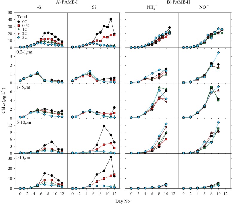
Time course of total and size fractionated Chl a concentrations in the (A) PAME-I mesocosms and the (B) PAME-II mesocosms.
Figure 4.
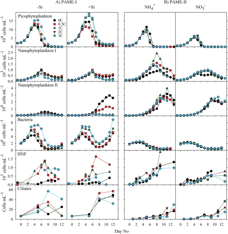
Time course of abundances in various osmo- and phago-trophic groups in the (A) PAME-I and (B) PAME-II mesocosms. The term picophytoplankton can include both eukaryotes and prokaryotes (mainly Synechococcus spp. and Prochlorococcus sp.). We did not detect any prokaryotes and hence the “picophytoplankton” is hereafter synonymous with picoeukaryotes.
Figure 6.
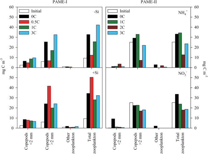
Initial (white bars) and final (colored bars where each color represent the different treatments) mesozooplankton community biomass in each mesocosm in PAME-I and PAME-II.
Results
Osmotrophs
The Chl a concentration was 1.07 μg L−1 when we started PAME-I. Addition of N and P initiated a phytoplankton bloom that culminated at 6.7–21.4 μg Chl a L−1 between day 6 and 8 in the −Si tanks, and at 5.9–40.6 μg Chl a L−1 between day 5 and 11 in the +Si tanks (Fig. 3). During the first four days total Chl a concentrations were similar in all tanks. From day 5 onward, the different silicate- and glucose enrichments promoted differences in the phytoplankton biomass development. Increasing glucose additions gave decreased Chl a concentrations in both gradients although most obvious in the Si amended one. The effect of reduced phytoplankton biomass with increased glucose supply was most evident in the two largest size fractions (5–10 μm and > 10 μm) which accounted for the majority (on average 60–100%) of the Chl a produced. Maximum phytoplankton biomass in the two smallest size fractions (0.2–1 μm and 1–5 μm) generally appeared prior to the main bloom (Fig. 3; Thingstad et al. 2008).
Compared to PAME-I, the most conspicuous traits of PAME-II with respect to Chl a is the small difference between treatments and continued increase in concentration throughout the experimental period (Fig. 3). The initial concentration was also lower (0.47 μg L−1). More than 70% of the phytoplankton biomass was produced in the 1–5 μm and 5–10 μm size fractions when integrated over the whole experimental period while the > 10 μm fraction played a minor role.
At the start of the PAME-I experiment, the abundance of picophytoplankton was 2 × 10⁴ cells mL−1 (Fig. 4). They bloomed and peaked at day 4–5 with highest density in the tanks receiving most glucose (3C). Maximum concentrations reached 1.2–1.5 × 10⁵ cells mL−1 in the −Si tanks and between 1.1–1.9 × 10⁵ cells mL−1 in the +Si amended tanks. Initial (ca., 0.7 × 10⁴ cells mL−1) and maximum picophytoplankton abundance was both lower in PAME-II than in PAME-I (Fig. 4). We did not observe any systematic variation along the glucose gradients in PAME-II but slightly higher maximum cell abundance in the compared to
 amended tanks (Fig. 4).
The initial concentrations of nanophytoplankton-I was approximately 1 × 10³ cell mL−1 in both experiments and reached maximum abundance on day 6 in PAME-I and on day 7–8 in PAME-II (Fig. 4). Maximum concentrations were about 1 × 10⁴ cells mL−1 in both gradients in PAME-I and in the gradient in PAME-II whereas they were somewhat higher and more variable in the
 amended gradient in PAME-II (0.9–2.4 × 10⁵ cell mL−1). There was no overall systematic effect of glucose enrichments on this phytoplankton group.
Silicate as well as glucose additions affected the diatom populations that totally dominated the nanophytoplankton-II in PAME-I (Fig. 5). Highest maximum concentrations were observed in the +Si tanks and decreased with increasing glucose addition in both gradients (Fig. 4). The diatom community was completely dominated by a small single celled Thalassiosira sp. (5–10 μm; Thingstad 2008). No diatom growth was observed in any enclosure in PAME-II despite Si additions to all. Instead, a 5–10 μm yellow flagellate resembling naked chrysophytes made up 75–89% of the nanophytoplankton-II community (percentage determined from FlowCAM data). Maximum concentrations were similar to maximum diatom cell number in PAME-I (yellow flagellate PAME-II: 4.0 × 10⁴ cell mL−1; diatoms PAME-I: 3.0 × 10⁴ cells mL−1). Highest abundances were observed between day 9 and 11 and did not vary systematically with glucose additions or N-source (Fig. 4).
Figure 5.
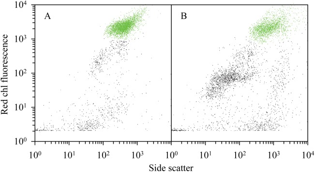
A water sample from tank 0C with added Si was enriched with Si-containing medium which promoted growth and complete dominance of a Thalassiosira species (see Thingstad et al. 2008, Supporting Information Fig. S5 for picture). The flow cytometry signatures of the Thalassiosira sp. in the enrichment culture (marked green in A) and the autotrophic nanoeukaryote population in tank 0C (marked green in B) were similar. Mean red chlorophyll fluorescence values (FL3) were 1931 for Thalassiosira in the enrichment culture and 1428 – 2728 for the autotrophic nanoeukaryotes in the mesocosms. The corresponding mean side-scatter values (SSC, indicating size and a very variable parameter for diatoms) were 419 and 789 – 953 respectively. This is strongly indicating that the autotrophic nanoeukaryote population in the mesocosms was dominated by the Thalassiosira sp. Further, a clonal Thalassiosira sp. isolate was produced from the enrichment culture and deposited in the culture collection at Department of Biology, University of Bergen. A phylogenetic analysis based on the small subunit (SSU) and partial large subunit (LSU) ribosomal ribonucleic acid (rRNA) gene sequences grouped the isolated Thalassiosira sp. with other species within the genus (Jensen 2012).
The initial concentration of bacteria was approximately 2 × 10⁶ mL−1 both years (Fig. 4). In PAME-I, the abundances of bacteria increased by a factor of 2–4 during the first 3–5 d in all tanks. The bacteria responded to the glucose addition by increased concentrations along the glucose gradient. In the −Si tanks, we observed one single maximum in bacterial abundance (around days 3–5), whereas the bacteria in the +Si amended tanks also increased substantially toward the end of the experiment. In the PAME-II experiment, the abundance of bacteria remained unchanged or increased slightly until day 3–4 (1.2–1.5 times the initial concentrations) before decreasing to less than initial values over a period of around seven days. The concentrations were similar in all tanks and independent of treatment.
Phagotrophs and grazing activity
The initial abundance of ciliates was higher and it started to increase earlier in PAME-I (average: 6 cells mL−1) than in PAME-II (0.4 cell mL−1) (Fig. 4). Maximum ciliate concentration was in general also higher in PAME-I (25–57 cells mL−1) than in PAME-II (between 6 and 37 cells mL−1). Preserving samples with pseudolugol may have led to underestimation of the microzooplankton abundance in PAME-I (Jakobsen and Carstensen 2011) and the difference between PAME-I and PAME-II may thus be underrated.
Although the initial abundance of HNF was higher in PAME-I than in PAME-II (Fig. 4), the HNF multiplied faster during PAME II than during PAME-I. In PAME-I, the abundance was much lower in the tanks without glucose additions than in the rest while in PAME-II increasing glucose addition had no discernable effect on the HNF abundance.
At the onset of PAME-I, the total mesozooplankton biomass (Fig. 6) was 10 mg C m−3 and consisted of a mixture of copepods > 2 mm (almost exclusively Calanus glacialis and Calanus finmarchicus), copepods < 2 mm (mainly Oithona spp.) plus a minor fraction of meroplanktonic larvae. During PAME-II, the initial mesozooplankton community was completely dominated by copepods > 2 mm (C. glacialis, C. finmarchicus), and the total biomass amounted to 25 mg C m−3 (Fig. 6). The average increase in total mesozooplankton biomass for all treatments from start to end was 3–4 times during PAME-I, whereas it remained at the same level or decreased during PAME-II (Fig. 6). There was no overall systematic effect of glucose enrichments on the mesozooplankton.
The initial grazing impact that the HNF and microzooplankton exerted on the bacteria (% daily removal of standing stock) was 1% during PAME-I and 27% during PAME-II (Fig. 7).
Figure 7.
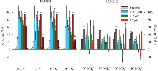
Effect of microzooplankton community grazing. The three vertical bars for each size fraction represent percent removal of standing stock per day of bacteria and different phytoplankton initially, early (day 2–5) and late (day 6–12) in the mesocosm experiments. Error bars are standard error (n = 6–10).
Grazing on bacteria increased throughout in both experiments but remained always higher in PAME-II than in PAME-I. There was no marked or systematic effect of nutrient treatment or glucose addition on grazing rates except for the high rate observed at the end of the experiment in the +Si amended tanks with high glucose (Fig. 7).
The initial grazing impact on the phytoplankton was much higher in PAME-I than in PAME-II, 84–94% and 14–35% of the standing stocks per day for all size classes, respectively (Fig. 7). Grazing on the smaller phytoplankton groups remained high throughout the experiment in PAME-I while grazing on the larger forms (> 5 μm) decreased. In PAME-II, there was an increased grazing on the smallest phytoplankton forms (0.22–1 μm) throughout while the results for the larger forms were more variable (Fig. 7). There was, however, no overall systematic effect of the different nutrient treatments or the glucose enrichments for any of the phytoplankton groups.
Model runs
In terms of the trophic structure of Fig. 1, the contrasting experimental outcomes in units with glucose and silicate in excess can be summarized as a dominance of bacteria (PAME-I) or flagellates (PAME-II), as opposed to the diatom response dominating in the MEDEA experiment (Thingstad et al. 2007). Experimental results analogous to the seven state variables of the model are shown in Fig. 8 and Table3, comparing the the 3C + Si (+NH4) unit in PAME-I and the 3C + NH4 (+Si) unit in PAME-II, both representative of units amended with excess glucose and silicate. Retaining the minimum philosophy used in constructing the original model, the smallest set of modifications we could find to adapt the model to the two PAME experiments consisted of (1) an introduction of ciliate grazing on the small diatoms in PAME-I, accompanied by a corresponding reduction in mesozooplankton clearance rate for diatoms; (2) different initial standing stocks of mesozooplankton (numerical values summarized in Table2). To allow direct comparison between model and experimental data, the set of fixed conversion factors was also expanded (Table2), but these do not affect model dynamics, only conversion from the model's phosphorous units to observed units such as abundances, Chl a, or carbon units. All other parameter values in the model were deliberately retained. With these modifications at the predator level, the large diatom bloom that dominated the model response for the MEDEA experiments is strongly reduced in PAME-I and disappears entirely in PAME-II (Fig. 8). The dominance of a continued bloom of autotrophic flagellates in PAME-II is now reproduced, as is the observed pattern for bacteria with higher abundance and a more dynamical response in PAME-I than in PAME-II (Fig. 8). The difference in the model's intial stock of mesozooplankton disappears at the end of the simulated experimental period, qualitatively in agreement with observations (Fig. 8). In the model, this is rooted in the assumption of a higher copepod clearance rate for ciliates than for diatoms, retained here from the original model. Otherwise, the key to understanding the different response patterns of the two PAME experiments lies in the opposite effect our two predator modifications has on ciliates. Allowing ciliates to feed on the small diatoms stimulates ciliate growth in PAME-I while the increased grazing from an initially higher mesozooplankton stock in PAME-II delays ciliate net increase until late in the experiment when their food has become abundant in the rising flagellate bloom (Fig. 8). The model reflects quite well the differences, both in pattern and level of observed ciliate abundances in PAME-I and PAME-II (Fig. 8; Table3). In the model, an increase in ciliate population induce cascades through two pathways: (1) via a decrease in heterotrophic flagellates into an increase in bacterial abundance, and also (2) through a decrease in autotrophic flagellates into an increase in free phosphate. Therefore, when bacterial growth is P-limited (i.e., C-replete), both abundance and growth rate of bacteria respond positively to an increase in ciliates. With these mechanisms, the model reproduces the observed rapid net growth in bacterial abundance toward the end of the experimental period for PAME-I and the lower and less dynamic bacterial abundance in PAME-II (Fig. 8).
Figure 8.
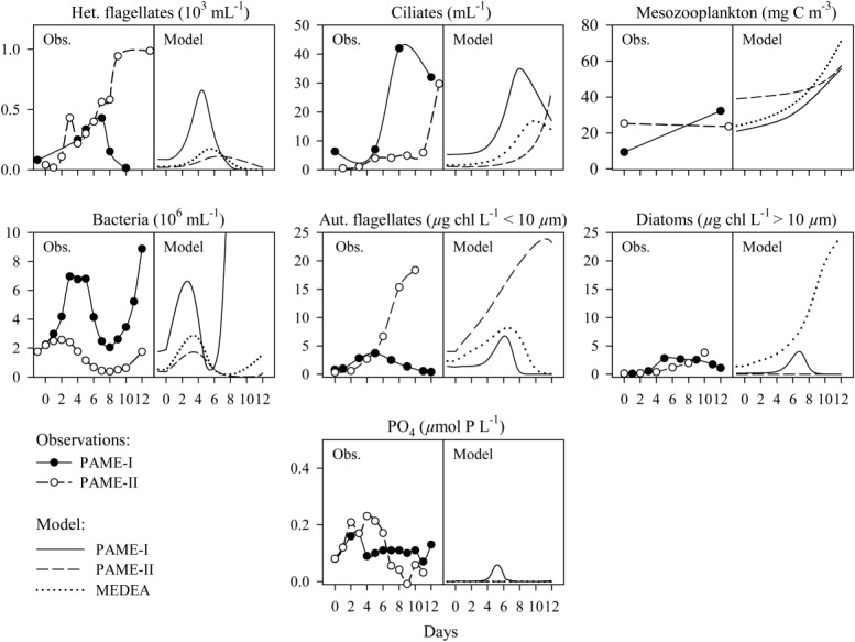
Observed (Obs.) and modeled (Model) responses for the mesocosm units with glucose (3 × C) and silicate (+Si) added in excess of biological consumption and ammonium as the nitrogen source for the PAME-I (solid lines) and PAME-II (broken lines) experiments. Variables arranged graphically to correspond to the model food web structure in Fig. 1. Model results for the MEDEA experiment (dotted lines) shown for comparison.
Table 3.
Qualitative and quantitative comparison between the model output and field observations (Obs.).
| Qualitative |
Quantitative |
||||||||
|---|---|---|---|---|---|---|---|---|---|
| PAME I |
PAME II |
PAME I |
PAME II |
||||||
| Obs. |
Model |
Obs. |
Model |
Obs. |
Model |
Obs. |
Model |
||
| Organism | Peak day no | Cells mL−1 | |||||||
| Het.bacteria | 1. Peak | 3 | 3 | 2 | 3 | 7×10⁶ | 6.6×10⁶ | 2.6×10⁶ | 1.7×10⁶ |
| 2. Peak | 12 | >8 | 12 | 12 | 9×10⁶ | >10×106 | 1.7×10⁶ | 0.3×10⁶ | |
| Het.flagellates | 1. Peak | 7 | 4 | 3 | 6 | 0.4×10³ | 0.6× 10³ | 0.4×10³ | 0.1×10³ |
| 2. Peak | – | – | 12 | – | – | – | 1.0×10³ | – | |
| Ciliates | 1. Peak | 8 | 8 | 12 | 12 | 42 | 35 | 30 | 27 |
| μg chl L−1 | |||||||||
| Diatoms (> 10 μm) | 1. Peak | 5 | 7 | 10 | 12 | 2.5 | 3 | 3 | 2.4×10⁻³ |
| Aut.flagellates (< 10 μm) | 1. Peak | 5 | 6 | 10 | 11 | 3.7 | 6.7 | 18 | 24 |
| μg C L−1 | |||||||||
| Mesozooplankton | Initial | 10 | 20 | 25 | 39 | ||||
| End | 33 | 55 | 24 | 57 | |||||
Discussion
A simple model—a complex issue
Figure 1 illustrates how the increase in resolution going from a simple food chain to a trophic network implies an extension of the one-dimensional “vertical” predator-prey balance contained in a traditional nutrient–phytoplankton–zooplankton model with a “horizontal” dimension representing the balance between alternative pathways. In the minimum model (Fig. 1), the horizontal dimension is simplified into three alternative pathways (bacteria, autotrophic flagellates, and diatoms). The division of the vertical dimension into three levels (nutrients, osmotrophs, and phagotrophs) is also a simplification as it ignores intermediate levels of mixotrophic protists (Zubkov and Tarran 2008; Mitra et al. 2014). Linking our 3 × 3 levels in the trophic “double pentagon” geometric structure of Fig. 1 determines how transients can move through the system while the numerical values of the parameters determines the charachteristic time scales of these transients. Although the model may appear overly simplisitic when compared to biological knowledge of the complexity of the real system, the dynamic balance in a 3 × 3 network is already a rather complex issue and the explanatory power of the model quite remarkable.
The dynamic part of the model is purely P-based, all other elements (e.g., O2 changes), compounds (e.g., chlorophyll), or cell abundances are calculated with fixed conversion factors from phosphorous. This implies that fluctuations at time scales where there are imbalances, e.g., between uptake of P, uptake of C, and cell division, are not captured by our minimum model. Such temporal decoupling is likely to occur between P-uptake and oxygen production and consumption. Biomass and cell abundances represent an integration of rates over time and thus tend to dampen out fluctuations in rate. This is reflected in our two alternative ways for calculating model O2-metabolism, where calculations based on rate and on biomass both give a reasonable level for GP and CR when compared to observations. The smoother response of the biomass-based calculations does however seem to better reflect the observed pattern, in particular for the PAME-I experiment (Fig. 9) and suggests that biomass-based calculations of C : P-coupling as used for diatom photosynthesis in the MEDEA experiment (Thingstad et al. 2007) may be a simple way to model the temporal decoupling between the P and C cycles.
Figure 9.
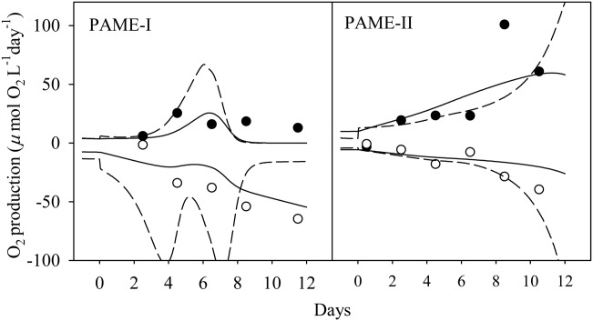
Observed gross production (filled circles) and community respiration (open circles) compared to modeled values based on O2-metabolism coupled P-uptake based (broken lines) and to biomass (solid lines) as outlined in Table2. Results for the mesocosm units with glucose (3 × C) and silicate (+Si) added in excess of biological consumption and ammonium as the nitrogen source in the PAME-I (left panel) and PAME-II (right panel) experiments.
Model explanatory power
The explanatory power of the model when applied to a single experiment and using one defined set of parameters was known from previous work (Thingstad et al. 2007). To what extent the structure and the parameter set used in a single case could be generalized to experiments in other environments was unknown, and the seemingly contrasting results obtained in the two PAME experiments could, at first sight, be taken as an indication of limited possibilities for such generalizations. Support for the idea that a relatively limited set of simple trophic connections dominate in the microbial food web can, however, be found in the litterature. Perturbing at the copepod level, Zöllner et al. (2009) demonstrated the validity of representing the link between copepods and bacteria with a linear trophic cascade through ciliates and heterotrophic flagellates as done in Fig. 1. Use of the right pentagon structure of Fig. 1 containing different grazers for the two phytoplankton groups also has experimental support in the work of Vadstein et al. (2004) who demonstrated how copepod grazing has opposite effects on chlorophyll levels depending on whether the phytoplankton community is dominated by flagellates or diatoms. Within the structure of Fig. 1, this is explained as the consequence of whether or not the phytoplankton-copepod connection has an intermediate ciliate link. Combining linear food chain from copepods to bacteria with the right pentagon structure and the mechanism giving phosphate limited bacteria when organic-C is in excess (Pengerud et al. 1987), gives the “double pentagon structure” of Fig. 1. Positioned in the upper right and upper left corner of the right and left pentagons, respectively, ciliates has a central position in the coupling of the two pentagons. The consequence is the key role of ciliates in controlling the model's response dynamics as explained in the Model runs-section.
A place where the model fails to produce a response reasonably similar to the data is in the phosphate concentrations (Fig. 8). There are several possible reasons for this. One is that the fixed stoichiometry used in the model does not allow for internal nutrient storage, which in nature may buffer oscillations in free phosphate concentrations of the type seen in the modeled response for PAME-I. Another complication is that the model operates only with phosphorous representing the limiting element. We added N and P in Redfield ratio and the system may well have been balancing on the border between N and P limitation. Comparisons between model and data is also complicated by the model output in the nanomolar range, below detection limit of our technique.
With more ciliates, the model gives a higher fractional loss for autotrophic flagellates in PAME-I than in PAME-II (not shown), reflecting the generally higher grazing rates observed on the three Chl a size fractions in PAME-I compared to PAME-II (Fig. 7). Measured predatory loss seems, however, to be less well represented. With a lower number of modeled heterotrophic flagellates in PAME-II (Fig. 8), the outcome is a lower fractional loss of bacteria. This is opposite to the observed trend with a higher bacterial loss rate to predators in PAME-II compared to PAME-I. Also, while the abundance of heterotrophic flagellates seems reasonably well reproduced for PAME-I this is not the case for PAME-II (Fig. 8; Table3). Whether the source for these discrepancies is in the model, or rooted in methodological limitations in the flow cytometer protocol used to count heterotrophic flagellates, is not known. It is interesting to note, however, that in the flagellate-dominated PAME-II experiment the heterotrophic flagellate counts follow the response pattern for Chl a < 10 μm (Fig. 8). With most autotrophic flagellates now believed to have phagotrophic capabilities (Mitra et al. 2014 and references therein) an intriguing possibility is that the model's separation of flagellates into an autotrophic and a heterotrophic group is biologically incorrect. The consequences of such an error, i.e., difference between modeled and observed HNFs, is larger for a phytoplankton community like in PAME-II when the flagellates totally dominated over diatoms. Merging flagellates into one mixotrophic group will, however, blur the left pentagon structure of our model. The consequences of this has not been explored, and the available methods to quantify mixotrophy in natural populations is still limited (discussed in Calbet et al. 2012).
The model indicates high degree of temperature resilience
It has been proposed that temperature reponses in the different functional groups of the pelagic food web may be different (Pomeroy and Deibel 1986; Rose and Caron 2007) and that the functionality of the system, therefore, may shift with temperature. The possibility to use a single set of parameters for simulating experiments 10°C apart does, however, not support the idea of major functional shifts within this temperature range. The impression is rather one of a resilient system when allowed to adapt to temperature. From the central role of ciliates in determining model dynamics at lower trophic levels, it follows that the model response would be quite sensitive to temperature effects at the ciliate level. The observations indicating that also this functional group seems to be populated by cold-adapted species in cold waters (Seuthe et al. 2011; Franzé and Lavrentyev 2014) is, therefore, interesting and supports our suggestions that the parameter set used may be valid over this temperature range without large temperature corrections. One could argue although that in a steady state situation, biomass values do not directly reflect rates and a steady state model may give correct biomasses with wrong rates. In a fluctuating system the net rates (growth − loss) must fluctuate correctly for the model to reproduce correct biomass fluctuations, a situation that can be illustrated by the oscillation observed in bacterial abundance in PAME-I (Fig. 8). In a classical Lotka–Volterra model with fixed predator growth rate μ and fixed predator loss rate δ, the period of oscillation is approximately and thus scales as the inverse of the geometric mean of the two specific rates. If the modeled period is correct with a wrong, e.g., a too high μ, this would need to be compensated by a too low modeled δ. A network of such interactions producing reasonably correct biomass fluctuations for the state variables with severely wrong rates seems rather difficult to construct, however. Based on our philosophy of making minimum changes to the original model, we did not add a temperature correction to the model's rate parameters. The oscillation in bacterial abundance in PAME-I (at ca., 7°C) has a period of ca., 10 d, as compared to the modeled period of ca., seven days. Assuming in analogy with the simple Lotka–Volterra equation that oscillation period scales as the inverse of a characteristic rate, this suggests that application of a Q10 around (7/10)−1 = 1.4 may be appropriate to convert the rate parameters originally fitted to the MEDEA system (ca., 17°C). This is lower than classical Q10 values in the range 1.9–2.2 (Eppley 1972 and references therein). Further confirmation of such a low temperature dependency would be important considering the potential consequences for our understanding of differences in microbial dynamics between Arctic and temperate systems.
The model emphasizes the structuring force of the mesozooplankton in the Arctic
The model's sensitivity to mesozooplankton grazing is an aspect with clear relevance to a changing Arctic. Altered seasonal migration of copepods (e.g., Hansen et al. 1998) caused by environmental changes, may create an imbalance between copepod standing stock and the microbial food supply. The copeod community of PAME-II was dominated by calanoid copepods > 2 mm, expected to feed preferentially on ciliates and large phytoplankton like diatoms (Calbet and Saiz 2005) as assumed in our model. In accordance with other studies showing maximum copepod population in Kongsfjorden in June (Kwasniewski et al. 2013), the initial copepod standing stock in the PAME-II mesocosms filled in late June was much higher than in PAME-I filled early August. The current results demonstrates the large impact such differences in copepod standing stock may have on the structure of Arctic microbial food webs.
The model and the osmotrophs
The double pentagon structure of our minimum model obviously lacks the resolution needed for comparison with all five groups of osmotrophs resolved in our data. Interestingly, however, there is a consistent temporal pattern in the observations with the abundance of smaller osmotrophs peaking before larger, i.e., in the sequence bacteria, pico-phytoplankton, nanophytoplankton I and then nanophytoplankton II (Fig. 4). The model gives such a pattern for the three osmotroph groups included and is primarily a consequence of the slower response assumed in larger predators. In particular, the inclusion of a separate functional group for autotrophic picoplankton would seem desireable and strengthen the model's applicability to oligotrophic environments, but exactly how one can include more phytoplankton groups in a manner reproducing the observed peak sequence, without at the same time destroying the desireable properties of the simple double pentagon structure, is not clear.
The intention of the experimental design of PAME-II was to test Stolte and Riegman's (1995) hypothesis for the role of ammonium and nitrate in determining the size structure of the diatom community. This test “failed” in the sense that no diatoms developed with either nitrogen source. Our model suggests an explanantion to why diatoms were suppressed, and also a suggested set of consequences when the diatom community are dominated by large- or small-celled species.
Concluding remarks
With data from to two experiments conducted at the Arctic location Kongsfjorden, Svalbard we demonstrate that a combination of mesocosm experimental work and modeling is most appropriate to reveal fundamental aspects of marine ecosystem functioning in relation to temperature adaptations as well as effects of mesozooplankton predators. The minimum mathematical model of the marine pelagic microbial food web, which was originally developed for temperate waters proved its ability to reproduce the empirical observed population dynamics in an 10°C colder, when taking into acoount initial differences at the preadator level. This emphasize a quite resilient microbial food web when adapted to in situ temperature, but also a strong mesozooplankton impact which emphasize the strong forcing function the seasonal vertical migration of copepods may have on Arctic microbial food webs. Another important lesson from the work presented here is the demonstration that apparently contrasting mesocosm results can be described as responses of a common model to moderate differences in initial conditions. The expensive consequence of this is that generalizations from a single mesocosm experiment should only be done with care, even when the experiment was done with an optimal set of controls, parallels, and factorial design. With three different observed response patterns explained within the framework of one model we feel, however, that the double-pentagon structure of Fig. 1 has a potential as a generic platform for further investigations of microbial trophodynamics.
Acknowledgments
The authors thank Kings Bay A/S and the staff at Ny Ålesund for help with the logistics.
This work was funded by the Research Council of Norway (RCN) through the International Polar Year Project “PAME-Nor” (IPY activity ID no. 71, RCN project no. 175939/S30), with additional support from the RCN project «MicroPolar: Processes and Players in Arctic Marine Pelagic Food Webs – Biogeochemistry, Environment and Climate Change” (RCN project no. 225956/E10); the MINOS project funded by EU-ERC (project no. 250254); the OCEAN-CERTAIN project funded by the European Commission (FP7-ENV-2013-6.1-1; no: 603773); and the core project BIOFEEDBACK of the Centre for Climate Dynamics (SKD) within the Bjerknes Centre for Climate Research. Support was also received from the Svalbard Science Forum as “Arktisstipend.”
References
- Aksnes DL. Cao FJ. Inherent and apparent traits in microbial nutrient uptake. Mar. Ecol. Prog. Ser. 2011;440:41–51. and. doi: 10.3354/meps09355. [Google Scholar]
- Alvarez E, Lopez-Urrutia A, Nogueira E. Fraga S. How to effectively sample the plankton size spectrum? A case study using FlowCAM. J. Plankton Res. 2011;33:1119−1133. and. doi: 10.1093/plankt/fbr012. [Google Scholar]
- Børsheim KY. Bacterial production rates and concentrations of organic carbon at the end of the growing season in the Greenland Sea. Aquat. Microb. Ecol. 2000;21:115–123. doi: 10.3354/ame021115. [Google Scholar]
- Calbet A. Saiz E. The ciliate-copepod link in marine ecosystems. Aquat. Microb. Ecol. 2005;38:157–167. and. doi: 10.3354/ame038157. [Google Scholar]
- Calbet A. Effects of light availability on mixotrophy and microzooplankton grazing in an oligotrophic plankton food web: Evidences from a mesocosm study in Eastern Mediterranean waters. J. Exp. Mar. Biol. Ecol. 2012;424–425:66–77. and others.. doi: 10.1016/j.jembe.2012.05.005. [Google Scholar]
- Eppley RW. Temperature and phytoplankton growth in the sea. Fish. Bull. 1972;70:1063–1085. [Google Scholar]
- Follows MJ, Dutkiewicz S, Grant S. Chisholm SW. Emergent biogeography of microbial communities in a model ocean. Science. 2007;315:1843–1846. doi: 10.1126/science.1138544. and. doi: 10.1126/science.1138544. [DOI] [PubMed] [Google Scholar]
- Franzé G. Lavrentyev PJ. Microzooplankton growth rates examined across a temperature gradient in the Barents Sea. Plos One. 2014 doi: 10.1371/journal.pone.0086429. 9 and : e86429. doi: 10.1371/journal.pone.0086429. [DOI] [PMC free article] [PubMed] [Google Scholar]
- Gaarder T. Gran HH. Investigations of the production of plankton in the Oslo Fjord. Rapp. Proc. Verb. Cons. Int. Explor. Mer. 1927;42:3–48. [Google Scholar]
- Hansen PJ, Bjørnsen PK. Hansen BW. Zooplankton grazing and growth: Scaling within the 2–2,000, um body size range. Limnol. Oceanogr. 1997;42:687–704. and. doi: 10.4319/lo.1997.42.4.0687. [Google Scholar]
- Hansen BW, Nielsen TG. Levinsen H. Plankton community structure and carbon cycling on the western coast of Greenland during the stratified summer situation. III Mesozooplankton. Aquat. Microb. Ecol. 1998;16:234–249. and. doi: 10.3354/ame016233. [Google Scholar]
- Harris GP. Temporal and spatial scales in phytoplankton ecology. Mechanisms, methods, models, and management. Can. Fish. Aquat. Sci. 1980;319:879–900. doi: 10.1139/f80-117. [Google Scholar]
- Havskum H. Silicate and labile DOC interfere in structuring the microbial food web via algal–bacterial competition for mineral nutrients: Results of a mesocosm experiment. Limnol. Oceanogr. 2003;48:129–140. and others.. doi: 10.4319/lo.2003.48.1.0129. [Google Scholar]
- Holmes RM, Aminot A, Kéroul R, Hooker AH. Peterson BJ. A simple and precise method for measuring ammonium in marine and freshwater ecosystems. Can. J. Aquat. Sci. 1999;56:1801–1808. [Google Scholar]
- Irigoien X, Flynn KJ. Harris RP. Phytoplankton blooms: A ‘loophole’ in microzooplankton grazing impact? J. Plankton Res. 2005;27:313–321. and. doi: 10.1093/plankt/fbi011. [Google Scholar]
- Jakobsen HH. Carstensen J. FlowCAM: Sizing cells and understanding the impact of size distributions on biovolume of planktonic community structure. Aquat. Microb. Ecol. 2011;65:75–87. and. doi: 10.3354/ame01539. [Google Scholar]
- Jensen TS. Phylogeny and functional studies of Thalassiosira. Univ. of Bergen, Norway; 2012. sp. isolated from Kongsfjorden, Svalbard. MSc thesis. [Google Scholar]
- Koroleff F. 1983. pp. 125–131. Methods of Seawater Analyses. K. Grasshoff, M. Ehrhardt, K. Kremling [eds.], 2nd, revised and extended edn. 419 pp. Weinheim/Deerfield Beach, Florida: Verlag Chemie.
- Kwasniewski S, Walkusz W, Cottier FR. Leu E. Mesozooplankton dynamics in relation to food availability during spring and early summer in a high latitude glaciated fjord (Kongsfjorden), with focus on Calanus. J. Mar. Syst. 2013;111–112:83–96. and. doi: 10.1016/j.jmarsys.2012.09.012. [Google Scholar]
- Landry MR. Estimating rates of growth and grazing mortality of photoautotrophic plankton by dilution. In: Cole JJ, editor; Kemp PF, Sherr BF, Sherr EB, editors. Handbook of methods in aquatic microbial ecology. Lewis Publishers; 1993. pp. 715–722. and [eds.], [Google Scholar]
- Larsen A. Population dynamics and diversity of phytoplankton, bacteria and virus in a seawater enclosure. Mar. Ecol. Prog. Ser. 2001;221:47–57. and others.. doi: 10.3354/meps221047. [Google Scholar]
- Le Quere C. Ecosystem dynamics based on plankton functional types for global ocean biogeochemistry models. Global Change Biol. 2005;11:2016–2040. and others.. doi: 10.1111/j.1365-2486.2005.1004.x. [Google Scholar]
- Marie D, Brussaard CPD, Thyrhaug R, Bratbak G. Vaulot D. Enumeration of marine viruses in culture and natural samples by flow cytometry. Appl. Environ. Microbiol. 1999;65:45–52. doi: 10.1128/aem.65.1.45-52.1999. [DOI] [PMC free article] [PubMed] [Google Scholar]
- Mitra A. The role of mixotrophic protists in the biological carbon pump. Biogeosciences. 2014;11:995–1005. and others.. doi: 10.5194/bg-11-995-2014. [Google Scholar]
- Montagnes DJS. Growth responses of planktonic ciliates in the genera Strobilidium and Strombidium. Mar. Ecol. Prog. Ser. 1996;130:241–254. doi: 10.3354/meps130241. [Google Scholar]
- Nejstgaard JC. Plankton development and trophictransfer in seawater enclosures with nutrients and Phaeocystis pouchetii added. Mar. Ecol. Prog. Ser. 2006;321:99–121. and others.. doi: 10.3354/meps321099. [Google Scholar]
- Parsons TR, Maita Y. Lalli CM. A manual of chemical and biological methods for seawater analysis. Pergamon Press; 1984. p. 173. [Google Scholar]
- Pengerud B, Skjoldal EF. Thingstad TF. The reciprocal interaction between degradation of glucose and ecosystem structure—studies in mixed chemostat cultures of marine-bacteria, algae, and bacterivorous nanoflagellates. Mar. Ecol. Prog. Ser. 1987;35:111–117. and. doi: 10.3354/meps035111. [Google Scholar]
- Pomeroy LR. Deibel D. Temperature regulation of bacterial activity during the spring bloom in Newfoundland coastal waters. Science. 1986;233:359–361. doi: 10.1126/science.233.4761.359. and. doi: 10.1126/science.233.4761.359. [DOI] [PubMed] [Google Scholar]
- Rose JM. Caron DA. Does low temperature constrain the growth rates of heterotrophic protists? Evidence and implications for algal blooms in cold waters. Limnol. Oceanogr. 2007;52:886–895. and. doi: 10.4319/lo.2007.52.2.0886. [Google Scholar]
- Seuthe L, Iversen KRokkan. Narcy F. Microbial processes in a high-latitude fjord (Kongsfjorden, Svalbard): II. Ciliates and dinoflagellates. Polar Biol. 2011;34:751–766. and. doi: 10.1007/s00300-010-0930-9. [Google Scholar]
- Sommer U. Comparison between steady state and non-steady state competition: Experiments with natural phytoplankton. Limnol. Oceanogr. 1985;30:335–346. doi: 10.4319/lo.1985.30.2.0335. [Google Scholar]
- Stibor H, Gelzleichter A, Hantzsche F, Sommer U, Striebel M, Vadstein O. Olsen Y. Combining dialysis and dilution techniques to estimate gross growth rate of phytoplankton and grazing by micro- and mesozooplankton in situ. Arch. Hydrobiol. 2006;167:403–404. and. doi: 10.1127/0003-9136/2006/0167-0403. [Google Scholar]
- Stibor H, Vadstein O, Lippert B, Roederer W. Olsen Y. Calanoid copepods and nutrient enrichment determine population dynamics of the appendicularian Oikopleura dioica: A mesocosm experiment. Mar. Ecol. Prog. Ser. 2004;270:209–215. and. doi: 10.3354/meps270209. [Google Scholar]
- Stock CA, Powell TM. Levin SA. Bottom–up and top–down forcing in a simple size-structured plankton dynamics model. J. Mar. Syst. 2008;74:134–152. and. doi: 10.1016/j.jmarsys.2007.12.004. [Google Scholar]
- Stolte W. Riegman R. Effect of a phytoplankton cell size on transient-state nitrate and ammonium uptake kinetics. Microbiology. 1995;141:1221–1229. doi: 10.1099/13500872-141-5-1221. and. doi: 10.1099/13500872-141-5-1221. [DOI] [PubMed] [Google Scholar]
- Thingstad TF. Cuevas LA. Nutrient pathways through the microbial food web: Principles and predictability discussed, based on five different experiments. Aquat. Microb. Ecol. 2010;61:249–260. and. doi: 10.3354/ame01452. [Google Scholar]
- Thingstad TF. Ability of a “minimum” microbial food web model to reproduce response patterns observed in mesocosms manipulated with N and P, glucose, and Si. J. Mar. Syst. 2007;64:15–34. and others.. doi: 10.1016/j.jmarsys.2006.02.009. [Google Scholar]
- Thingstad TF. Counterintuitive carbon-to-nutrient coupling in an Arctic pelagic ecosystem. Nature. 2008;455:387–391. doi: 10.1038/nature07235. and others. doi: 10.1038/nature07235. [DOI] [PubMed] [Google Scholar]
- Tilman D, Kilham SS. Kilham P. Phytoplankton community ecology: The role of limiting nutrients. Annu. Rev. Ecol. Syst. 1982;13:349–372. and. doi: 10.1146/annurev.es.13.110182.002025. [Google Scholar]
- Vadstein O, Andersen T, Reinertsen HR. Olsen Y. Carbon, nitrogen and phosphorus resource supply and utilisation for coastal planktonic heterotrophic bacteria in a gradient of nutrient loading. Mar. Ecol. Prog. Ser. 2012;447:55–75. and. doi: 10.3354/meps09473. [Google Scholar]
- Vadstein O. Moderate increase in the biomass of omnivorous copepods may ease grazing control of planktonic algae. Mar. Ecol. Prog. Ser. 2004;270:199–207. and others.. doi: 10.3354/meps270199. [Google Scholar]
- Valderrama JC. Manual on HARMFUL Marine Microalgae. In: Cembella AD, editor; Hallegraeff GM, Anderson DM-, editors. IOC Manuals and Guides number 33. UNESCO; 1995. pp. 262–265. and [eds.], [Google Scholar]
- Verity PG. Villareal TA. The relative food value of diatoms, dinoflagellates, flagellates and cyanobacteria for tintinnid cultures. Archiv Protistenk. 1986;131:71–84. and. doi: 10.1016/S0003-9365(86)80064-1. [Google Scholar]
- Verity PG, Whipple SJ, Nejstgaard JC. Alderkamp A-C. Colony size, cell number, carbon and nitrogen contents of Phaeocystis pouchetii from western Norway. J. Plankton Res. 2007;29:359–367. and. doi: 10.1093/plankt/fbm021. [Google Scholar]
- Zubkov M, Burkill PH. Topping JN. Flow cytometric enumeration of DNA-stained oceanic planktonic protists. J. Plankton Res. 2007;29:79–86. and. doi: 10.1093/plankt/fbl059. [Google Scholar]
- Zubkov MV. Tarran GA. High bacterivory by the smallest phytoplankton in the North Atlantic Ocean. Nature. 2008;455:224–226. doi: 10.1038/nature07236. and. doi: 10.1038/nature07236. [DOI] [PubMed] [Google Scholar]
- Zöllner E, Hoppe HG, Sommer U. Jürgens K. Effect of zooplankton-mediated trophic cascades on marine microbial food web components (bacteria, nanoflagellates, ciliates) Limnol. Oceanogr. 2009;54:262–275. and. doi: 10.4319/lo.2009.54.1.0262. [Google Scholar]