Separating the influence of temperature, drought, and fire on interannual variability in atmospheric CO₂

Abstract

The response of the carbon cycle in prognostic Earth system models (ESMs) contributes significant uncertainty to projections of global climate change. Quantifying contributions of known drivers of interannual variability in the growth rate of atmospheric carbon dioxide (CO₂) is important for improving the representation of terrestrial ecosystem processes in these ESMs. Several recent studies have identified the temperature dependence of tropical net ecosystem exchange (NEE) as a primary driver of this variability by analyzing a single, globally averaged time series of CO₂ anomalies. Here we examined how the temporal evolution of CO₂ in different latitude bands may be used to separate contributions from temperature stress, drought stress, and fire emissions to CO₂ variability. We developed atmospheric CO₂ patterns from each of these mechanisms during 1997–2011 using an atmospheric transport model. NEE responses to temperature, NEE responses to drought, and fire emissions all contributed significantly to CO₂ variability in each latitude band, suggesting that no single mechanism was the dominant driver. We found that the sum of drought and fire contributions to CO₂ variability exceeded direct NEE responses to temperature in both the Northern and Southern Hemispheres. Additional sensitivity tests revealed that these contributions are masked by temporal and spatial smoothing of CO₂ observations. Accounting for fires, the sensitivity of tropical NEE to temperature stress decreased by 25% to 2.9 ± 0.4 Pg C yr⁻¹ K⁻¹. These results underscore the need for accurate attribution of the drivers of CO₂ variability prior to using contemporary observations to constrain long-term ESM responses.

Key Points

• Accurate attribution of CO₂ variability is required to constrain coupled models

• Combined influence of drought and fire exceed ecosystem responses to temperature

• Temporal and spatial smoothing of CO₂ observations masks variability from fire

1 Introduction

Observed variations in the growth rate of atmospheric carbon dioxide, CO₂, provide insight about the processes that govern land and ocean sinks for anthropogenic CO₂. Interannual variability in atmospheric CO₂ is tightly linked with volcanic eruptions [Farquhar and Roderick, ²⁰⁰³; Frölicher et al., ²⁰¹³] and climate modes, including El Niño–Southern Oscillation (ENSO) [Bacastow, ¹⁹⁷⁶; Jones et al., ²⁰⁰¹; Zeng et al., ²⁰⁰⁵; Schwalm et al., ²⁰¹¹]. Evidence from carbon isotopes suggests that these CO₂ variations originate mostly from terrestrial ecosystems, rather than ocean carbon exchange [Francey et al., ¹⁹⁹⁵; Battle et al., ²⁰⁰⁰; Rayner et al., ²⁰⁰⁸; Alden et al., ²⁰¹⁰].

Recent work has improved our understanding of the underlying processes regulating variability in carbon fluxes within terrestrial ecosystems. Many studies have noted a positive correlation between land temperature anomalies and the atmospheric CO₂ growth rate [Keeling et al., ¹⁹⁹⁵; Braswell, ¹⁹⁹⁷; Rafelski et al., ²⁰⁰⁹], especially during the warm El Niño phase of ENSO [Wang et al., ²⁰¹³]. Tropical ecosystem responses to warmer temperature tend to release CO₂ to the atmosphere as a consequence of several physiological processes that operate in concert. Specifically, gross primary production (GPP) in tropical forests generally decreases in response to lower carboxylation efficiency and other stresses [Berry and Bjorkman, ¹⁹⁸⁰; Doughty and Goulden, ²⁰⁰⁸]. Autotrophic respiration responses also likely contribute to carbon losses as a consequence of greater leaf, stem, and root maintenance costs. In parallel, microbial responses to higher temperature cause decomposition to accelerate [Atkin, ²⁰⁰³; Davidson and Janssens, ²⁰⁰⁶; Mahecha et al., ²⁰¹⁰], increasing emissions from litter and soil organic matter. These plant and microbial responses to temperature are widely represented in terrestrial ecosystem models, albeit with varying temperature dependencies [Todd-Brown et al., ²⁰¹³]. We hereafter refer to the combined set of these canopy-scale processes (and their temperature dependencies) as the direct temperature response of net ecosystem exchange (NEE); alone, this response is sufficient to generate a strong positive relationship between interannual temperature variations and tropical CO₂ fluxes in models [Wang et al., ²⁰¹³].

Climate modes also modify hydrology, complicating explanations of atmospheric CO₂ variability that rely solely on NEE responses to temperature. Shifts in atmospheric circulation from Pacific or Atlantic sea surface temperature anomalies modify rainfall in tropical and subtropical terrestrial ecosystems [Ropelewski and Halpert, ¹⁹⁸⁷; Nobre and Shukla, ¹⁹⁹⁶]. In certain wet tropical forests, seasonal or interannual drought reduces soil respiration considerably, whereas GPP may be less affected as a consequence of increased light availability and the ability of deeply rooted trees to withstand desiccation of surface soil layers [Saleska et al., ²⁰⁰³; Bonal et al., ²⁰⁰⁸]. Due to a paucity of data, it remains unclear how tropical drought responses vary along moisture gradients or with vegetation type; however, top-down constraints from atmospheric CO₂ suggest that in the Amazon, basin-wide net carbon uptake is reduced in drought years [Gatti et al., ²⁰¹⁴]. In temperate ecosystems, eddy covariance observations likewise indicate that, overall, drought-induced reductions in GPP exceed those for ecosystem respiration, and therefore, net carbon uptake is reduced [Schwalm et al., ²⁰¹⁰].

In addition to the temperature and drought stress impacts on NEE described above, fires also contribute to atmospheric CO₂ variability on interannual time scales. Fire emissions are usually confined to the dry season in tropical forests and are regulated both by climate and human drivers [van der Werf et al., ²⁰¹⁰; Bowman et al., ²⁰¹¹]. In savannas, drought conditions often increase burning in woodlands but reduce fuel availability and emissions in drier grasslands [Randerson et al., ²⁰⁰⁵]. Fires also contribute to interannual variability in atmospheric methane (CH₄) [Bousquet et al., ²⁰⁰⁶] and are a dominant driver of interannual variability in carbon monoxide (CO) [Langenfelds et al., ²⁰⁰²; van der Werf et al., ²⁰⁰⁴]. When CH₄ and CO observations are combined with measurements of emission ratios from smoke plumes [Andreae and Merlet, ²⁰⁰¹; Akagi et al., ²⁰¹¹], they provide evidence for a significant contribution from fires to variability in atmospheric CO₂ [Langenfelds et al., ²⁰⁰²; van der Werf et al., ²⁰⁰⁴; Gatti et al., ²⁰¹⁴].

Partitioning the observed variability in atmospheric CO₂ to temperature, drought, and fire drivers remains an important research challenge because the correct balance of mechanisms is needed to simulate the global carbon cycle accurately in Earth system models (ESMs). Recently, Wang et al. [2013] found that the temperature sensitivity of tropical NEE was the dominant mechanism explaining CO₂ interannual variability, with considerably weaker controls from precipitation-induced changes in NEE and even smaller contributions from fires. Similarly, Cox et al. [2013] found that heterotrophic respiration responses in C4MIP models were the primary drivers of model-to-model differences in the sensitivity of tropical NEE to temperature, with no explicit estimate of fire emissions considered in model comparisons with observations. In both studies, the CO₂ record used in the analysis was a globally averaged time series that was further temporally smoothed during estimation of the growth rate, either by using a 12 month running mean [Wang et al., ²⁰¹³] or by differencing the annual means from two consecutive years [Cox et al., ²⁰¹³].

Here we examined how higher-resolution atmospheric CO₂ data may improve the attribution process. An important motivation was the observation that many of the climate extremes over the last several decades have been confined to specific regions [Reichstein et al., ²⁰¹³], and thus, biospheric responses to these events likely leave an asymmetric (and unique) imprint on the meridional distribution of CO₂. In addition, emission anomalies from fires are phase locked to the dry season in tropical forests and are closely associated with regional hotspots of land use change, further enabling separation of this tracer from NEE responses to temperature and drought stress.

In section 2, we describe our method to simulate interannual variability in atmospheric CO₂ from simple basis fluxes derived from gridded climate data. These basis fluxes were propagated through an atmospheric transport model [Suntharalingam et al., ²⁰⁰⁴; Nassar et al., ²⁰¹⁰], enabling direct comparison of simulated CO₂ against meridional and temporal patterns in monthly atmospheric observations. In section 3, we present the relative contribution of individual drivers and combinations thereof to the observed interannual variability of CO₂ during 1997–2011 determined from optimal estimation. In section 4, we discuss how the interplay among these drivers provides both improved estimates of the climate sensitivity of NEE and directions for reducing carbon cycle uncertainties in ESMs.

2 Data and Methods

2.1 Atmospheric CO₂ Observations

We analyzed CO₂ interannual variability for the 15 year period from 1997 through 2011 using monthly mean NOAA global cooperative air sampling network observations [Dlugokencky et al., ²⁰¹³] at marine boundary layer (MBL) sites with greater than 70% data coverage for the time period of interest (Figures 1a–1f and Table 1). We chose this period based on the availability of fire emissions data [van der Werf et al., ²⁰¹⁰] to compare with temperature and drought effects. CO₂ interannual variability was calculated by (1) detrending the observed time series at each site with a third-order polynomial, (2) computing a mean annual cycle from the detrended time series, (3) removing the mean annual cycle from the original time series, and (4) fitting a third-order polynomial to the time series obtained from step (3) [Keppel-Aleks et al., ²⁰¹³]. Our results were largely insensitive to the method of calculating the monthly mean CO₂ or to detrending methodology (data not shown). We averaged the CO₂ time series into six bands encompassing the tropics, midlatitude, and high latitude in each hemisphere for comparison with simulated CO₂ response functions (Figures 1g–1l). Although the resulting time series for CO₂ variability share similarities, each band is influenced by a different mix of local and remote fluxes modified by atmospheric transport.

Figure 1.

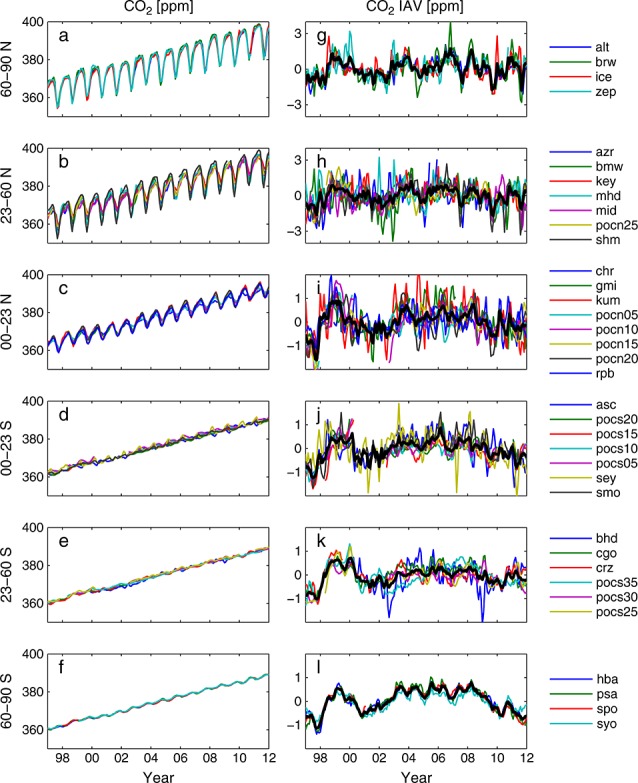
Observations of atmospheric CO₂ from 1997 to 2011 in different latitude bands. (a–f) Original monthly mean time series and (g–l) the interannual component of atmospheric CO₂ variations from marine boundary layer (MBL) sites in the NOAA ESRL global cooperative air sampling network. Observations were binned into six latitude bands for comparison with simulated CO₂. Station acronyms and location information appear in Table 1.

Table 1.

Marine Boundary Layer (MBL) Sites in NOAA's Global Cooperative Air Sampling Network

Region	Station	Acronym	Latitude [°N]	Longitude [°E]
60–90°N	Alert, Nunavut, Canada	ALT	82.5	−62.5
	Ny Ålesund, Svalbard	ZEP	78.9	11.9
	Barrow, Alaska	BRW	71.3	−156.6
	Storhofdi, Iceland	ICE	63.4	−20.1
23–60°N	Mace Head, Ireland	MHD	53.3	−9.9
	Shemya, Alaska	SHM	52.7	174.1
	Terceira Island, Azores	AZR	38.8	−27.4
	Tudor Hill, Bermuda	BMW	32.3	−64.7
	Midway Island	MID	28.2	−177.4
	Key Biscayne, Florida	KEY	25.7	−80.2
	Pacific Ocean 25°N	POCN25	25.0	−139.0
0–23°N	Pacific Ocean 20°N	POCN20	20.0	−141.0
	Cape Kumukahi, Hawaii	KUM	19.5	225.0
	Pacific Ocean 15°N	POCN15	15.0	−145.0
	Mariana Islands, Guam	GMI	13.4	144.8
	Ragged Point, Barbados	RPB	13.2	−59.4
	Pacific Ocean 10°N	POCN10	10.0	−149.0
	Pacific Ocean 5°N	POCN05	5.0	−151.0
0–23°S	Mahe Island, Seychelles	SEY	−4.7	55.2
	Pacific Ocean 5°S	POCS05	−5.0	−159.0
	Ascension Island	ASC	−8.0	−14.4
	Pacific Ocean 10°S	POCS10	−10.0	−161.0
	Tutuila, American Samoa	SMO	−14.3	−170.6
	Pacific Ocean 15°S	POCS15	−15.0	−171.0
	Pacific Ocean 20°S	POCS20	−20.0	−174.0
23–60°S	Pacific Ocean 25°S	POCS25	−25.0	−171.0
	Pacific Ocean 30°S	POCS30	−30.0	−176.0
	Pacific Ocean 35°S	POCS35	−35.0	−180.0
	Cape Grim, Tasmania	CGO	−40.7	144.7
	Baring Head, New Zealand	BHD	−41.0	174.0
	Crozet Island	CRZ	−46.5	51.9
60–90°S	Palmer Station, Antarctica	PSA	−64.0	−64.0
	Syowa, Antarctica	SYO	−69.0	39.6
	Halley Bay, Antarctica	HBA	−75.6	−26.5
	South Pole	SPO	−90.0	−24.8

2.2 Atmospheric CO₂ Simulated From Simple Basis Fluxes

We simulated monthly mean CO₂ patterns arising from prescribed fluxes using the GEOS-Chem atmospheric transport model, version 9.1.2 [Suntharalingam et al., ²⁰⁰⁴; Nassar et al., ²⁰¹⁰]. The model was driven by 3- to 6-hourly Modern Era Retrospective-Analysis for Research and Applications reanalysis meteorology [Rienecker et al., ²⁰¹¹] at 4° (latitude) by 5° (longitude) horizontal resolution with 47 vertical layers. We sampled monthly mean model output at the grid cells containing the MBL sites, and we detrended and binned simulated CO₂ identically to the observations. CO₂ response functions from individual basis fluxes were carried as individual tracers.

We used spatially resolved monthly climate time series to construct a series of NEE sensitivity basis fluxes without closely tying our results to the parameterizations of any specific ecosystem model (Figure 2). These fluxes were uniform across an entire month. To represent the influence of temperature stress on NEE, we used land air temperature anomalies at 5° by 5° resolution from the Climatic Research Unit (CRU) at the Hadley Centre [Jones et al., ²⁰¹²]. We modeled the interannually varying component of the NEE flux due to temperature variations (NEE_T) as follows:

1

where the temperature anomaly at each grid cell from its monthly long-term mean () is scaled by the annually integrated net primary production (NPP), following the assumption that the magnitude of monthly NEE anomalies at a particular location should be proportional to gross ecosystem fluxes at the same location. In equation (1), t represents time (year and month), while m represents month of the year for the long-term temperature climatology, x represents latitude, and y represents longitude. For the gridded annual mean NPP fluxes we used a climatological estimate derived from the Carnegie-Ames-Stanford Approach (CASA) biogeochemical model at a 1° by 1° resolution [Randerson et al., ¹⁹⁹⁷]. Given the high degree of spatial correlation of annual NPP from models derived from satellite estimates of the fraction of absorbed photosynthetically active radiation and that we only used NPP to scale the spatial pattern of time-evolving NEE anomalies, the results we present have only a marginal sensitivity to specific parameterizations within the biogeochemical model. We included an exponential term (Q₁₀ = 2) that reduced the impact of temperature anomalies at colder temperatures. The normalization constant κ_T was determined such that the standard deviation in annually integrated NEE_T was 1 Pg C yr⁻¹ globally over 15 years.

Figure 2.

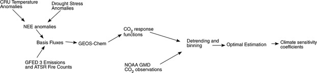
Flow chart for optimal estimation of model parameters and climate sensitivity coefficients.

This model assumes that NEE variations on interannual time scales can be represented as a linear perturbation of temperature anomalies, with the magnitude of the response proportional to the gross ecosystem fluxes in a given region. Although ecosystems may exhibit nonlinear or threshold responses to temperature or drought stress [Berry and Bjorkman, ¹⁹⁸⁰; Reichstein et al., ²⁰¹³], we caution that discriminating and fitting such nonlinear responses within the 15 year duration of our study period would lead to a loss in the robustness of our results given the required increase in the number of fitting parameters and degrees of freedom. Analysis of nonlinear climate impacts on terrestrial ecosystem fluxes may better be suited for future analysis when longer global time series of fire emissions and ecosystem fluxes permit the use of more sophisticated statistical models.

Similarly, we developed a family of basis fluxes to represent the impact of drought stress (D) on NEE (NEE_D) using three drivers that reflect moisture stress on different time scales. We used precipitation from the Global Precipitation Climatology Project (GPCP) [Adler et al., ²⁰⁰³], which reflects the short-term water inputs to the ecosystem. We also used two metrics from NCEP reanalysis climatology [Kalnay et al., ¹⁹⁹⁶]: Palmer Drought Severity Index (PDSI) [Dai et al., ²⁰⁰⁴], which reflects the cumulative departure from local moisture balance, and potential evaporation (PE), which reflects the evaporative demand given a sufficient soil water source. We used a similar framework to estimate the perturbation to NEE (NEE_D) from drought stress (D) for each of these proxies:

2

As in equation (1), κ_D was a normalization constant such that each gridded NEE_D time series had a global standard deviation of 1 Pg C yr⁻¹ from 1997 to 2011. For this convention, CO₂ fluxes were positive to the atmosphere when precipitation had a positive deviation relative to climatology and when PDSI was in a positive phase (indicating water abundance).

For fires, we used emissions from the Global Fire Emissions Database (GFED3) [van der Werf et al., ²⁰¹⁰], which combines satellite observations of active fire counts, burned area, and vegetation productivity with the CASA biogeochemical model to calculate fire emissions. We also prescribed a mostly independent set of fire emissions scaled according to the Along-Track Scanning Radiometer (ATSR) distribution of active fires [Arino and Melinotte, ¹⁹⁹⁸]. Because ATSR is a polar-orbiting satellite and therefore oversamples fires at high latitudes relative to midlatitude and tropical fires, we scaled the ATSR fire counts in 10° latitude bins by the fraction of GFED emissions occurring within each bin, thus imposing GFED's latitudinal emissions distribution while preserving distinct patterns of variability between the two basis flux sets.

2.3 Optimal Estimation

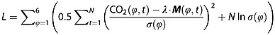
Simulated CO₂ response functions from global and regional fluxes were compared against observed interannual variability either individually or in linear combination. We determined scale factors, λ, for each driver included in the model by minimizing the cost function:

3

In equation (3), CO₂ (ϕ,t) is the observed interannual variability in each latitude band, ϕ. The matrix M(ϕ,t) contains the individual CO₂ response functions simulated by GEOS-Chem from driver fluxes with 1 Pg C yr⁻¹ standard deviation. The vector λ contains the optimal scale factors that modulate the standard deviation of the fluxes in each model case. We did not expect that our simple flux models would account for all variability across each latitude band. In the Northern Hemisphere, for instance, observations were characterized by greater temporal variability that likely owes to contributions from fossil fuel fluxes and other processes that were not resolved in our modeling framework. We therefore simultaneously fit parameters σ(ϕ) to represent the unresolved variability in each latitude band. Their optimal values reflect the balance between the sum-squared residual and penalty terms of the cost function that resulted in each latitude band contributing equally to the overall sum-squared residual. Our optimizations were conducted without prior constraints on the fluxes. To account for correlations among successive months, we determined the effective number of CO₂ observations in each latitude band assuming an autoregressive (AR1) model and inflated the posterior error covariance matrix by the ratio of actual to effective sample size. We tested the sensitivity of the results to different cost function formulations by weighting the six latitude bands by area fraction and by assuming a t distribution for errors. In each case, the optimized λ values remained within the reported error bars, demonstrating the robustness of the optimization results presented in section 3.

We assessed the quality of our regression models for each latitude band using both the familiar Pearson's R² coefficient (which indicates the degree of correspondence between model and data) and the RMS amplitude factor. The amplitude factor, A, was calculated as a ratio of the standard deviation in the simulated CO₂ time series (adjusted by the appropriate λ values) to the standard deviation in the observed CO₂ time series (equation (4)) and therefore provides information about the magnitude of variability explained by each flux model.

4

We used the F test to compare the relative performance of different regression models; for this test, the number of data was adjusted by the effective sampling rate calculated from the AR1 model. We also used posterior predictive model checking [Gelman et al., ¹⁹⁹⁶] to test whether synthetic CO₂ data generated from our optimized regression models reproduced the observed correlations among temperature, drought, and fire. This provides a quality metric that focuses specifically on the ability to faithfully attribute signal to each driver, rather than just reflecting the overall goodness of fit as given by the R² coefficient. This model comparison was carried out by fitting synthetic data using single-driver, single-region regression models and by comparing the resulting λ values to those determined from fits to the observations themselves.

3 Results

CO₂ fluxes from temperature, drought, and fire emissions captured many of the large-scale features in observed atmospheric CO₂ variability from 1997 to 2011 (Figure 3). Contributions from fossil [Andres et al., ²⁰¹¹] and ocean fluxes [Doney et al., ²⁰⁰⁹] (Figure 3b) were relatively small across all latitudes and consistent with earlier work [Bousquet et al., ²⁰⁰⁰; Nevison et al., ²⁰⁰⁸; Rayner et al., ²⁰⁰⁸]. We optimized scale factors (λ) for each of the terrestrial CO₂ response functions using single-factor regression models (Table 2). Since the CO₂ response functions were simulated from flux fields normalized to 1 Pg C yr⁻¹ standard deviation, the values of λ can be interpreted as the standard deviation of the optimized carbon fluxes (in units of Pg C yr⁻¹) owing to individual climate drivers over the 15 year period.

Figure 3.

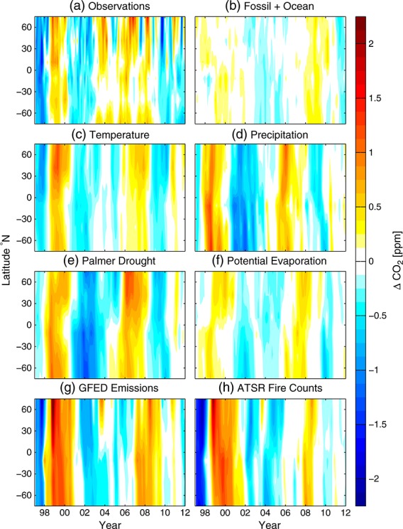
Hovmöller diagrams for observed and simulated CO₂ interannual variability. (a) Observed variability determined from MBL sites (Figure 1 and Table 1). (b) CO₂ response functions derived from the sum of fossil fuel and ocean fluxes. (c) CO₂ response function derived from the temperature sensitivity of NEE. CO₂ response functions derived from the drought sensitivity of NEE determined from (d) precipitation, (e) Palmer Drought Severity Index (PDSI), and (f) potential evaporation (PE). The CO₂ patterns arising from drought stress metrics were scaled by −1, since the simulated patterns were negatively correlated with the observations. CO₂ response functions from fire emissions from (g) the Global Fire Emissions Database version 3 (GFED3) and (h) scaled Along Track Scanning Radiometer (ATSR) fire counts. X axis tick marks and year labels correspond to the beginning of each calendar year.

Table 2.

The Contribution of Terrestrial Ecosystem Fluxes to Interannual Variability in Atmospheric CO₂ From Single-Variable Global Flux Models^a

	Global		60–90°N		23–60°N		0–23°N		0–23°S		23–60°S		60–90°S
	R2	A	R2	A	R2	A	R2	A	R2	A	R2	A	R2	A	λ
Temperature	0.46	0.61	0.33	0.57	0.25	0.67	0.47	0.65	0.50	0.58	0.60	0.66	0.63	0.52	0.80 ± 0.07
PDSI	0.42	0.55	0.24	0.40	0.31	0.44	0.39	0.49	0.41	0.63	0.66	0.73	0.48	0.60	−0.47 ± 0.05
GFED3	0.36	0.51	0.24	0.44	0.24	0.44	0.41	0.52	0.32	0.57	0.58	0.62	0.35	0.49	0.40 ± 0.05
ATSR	0.34	0.51	0.24	0.38	0.25	0.43	0.42	0.51	0.35	0.57	0.52	0.64	0.26	0.51	0.37 ± 0.05
Precipitation	0.34	0.47	0.18	0.29	0.26	0.34	0.30	0.43	0.28	0.57	0.48	0.64	0.53	0.54	−0.44 ± 0.05
PE	0.20	0.38	0.11	0.25	0.08	0.30	0.15	0.33	0.19	0.42	0.31	0.53	0.38	0.44	0.67 ± 0.13

^aThe Pearson's R² coefficient and the amplitude factor (A), calculated as the ratio of the simulated CO₂ standard deviation to the observed CO₂ standard deviation, are shown for each model. The scale factor (λ) was optimized for each model to minimize the cost function across all six latitude bands. All reported errors represent standard deviations.

Among individual terrestrial ecosystem drivers, the temperature-driven NEE model was positively correlated with the observed CO₂ patterns and explained the largest amount of variance across different latitude bands with an average R² of 0.46. After optimization, the temperature-driven NEE fluxes had a standard deviation of 0.80 ± 0.07 Pg C yr⁻¹ and the adjusted atmospheric CO₂ response function had a standard deviation that was 61% relative to that of the observations (Table 2).

The CO₂ response function from NEE responding to the Palmer Drought Severity Index (PDSI) had the second most explanatory power with a mean R² of 0.42 and an adjusted standard deviation (hereafter termed the amplitude factor) that was 55%. The CO₂ patterns arising from PDSI and precipitation were negatively correlated with the observations, indicating that drought stress increased CO₂ growth and decreased terrestrial carbon storage on interannual time scales. The two fire emissions time series, GFED3 and ATSR, were the third most important class of models, with mean R² values of 0.36 and 0.34, respectively, and each with an amplitude factor of 51% of the observations. The optimized GFED3 flux standard deviation of 0.40 ± 0.05 Pg C yr⁻¹ was 25% higher than the standard deviation of the original GFED3 emissions time series (0.32 Pg C yr⁻¹) but within expected uncertainties [van der Werf et al., ²⁰¹⁰]. Although the precipitation and potential evaporation (PE) CO₂ patterns were qualitatively similar to PDSI (Figures 3d–3f), the mean R² was only 0.34 for precipitation and 0.20 for PE, in part due to a likely time delay in NEE responses to precipitation anomalies [Zeng et al., ²⁰¹³].

To isolate the contribution of tropical fluxes to atmospheric CO₂ variability, we ran an additional GEOS-Chem simulation for each of the drivers described above, considering only fluxes between 23°N and 23°S. The CO₂ variability explained by tropical NEE fluxes had similar Pearson's R² coefficients as the global models even in the extratropics (Table 3), confirming earlier work showing that tropical ecosystem responses to climate influence CO₂ variability globally [Bousquet et al., ²⁰⁰⁰; Rayner et al., ²⁰⁰⁸]. A key mechanism explaining this result is the coupling of large net ecosystem carbon flux anomalies to tropical deep convection that efficiently transports these fluxes poleward in the upper troposphere [Plumb and Mahlman, ¹⁹⁸⁷]. With the exception of fire emissions, regression models derived from extratropical Northern Hemisphere fluxes had considerably lower performance metrics than their tropical or global counterparts (Table 4), while extratropical Southern Hemisphere fluxes had almost no impact on CO₂ variability globally (Figure 4). Northern Hemisphere fires explained a much larger fraction of the CO₂ variability at northern middle and high latitudes than tropical or global fires, consistent with past studies documenting considerable interannual variability in boreal forest fires [Kasischke et al., ²⁰⁰⁵] and the proximity of northern surface stations to these sources.

Table 3.

The Contribution of Terrestrial Ecosystem Fluxes to Interannual Variability in Atmospheric CO₂ From Single-Variable Tropical Flux Models, Similar to Table 2

	Global		60–90°N		23–60°N		0–23°N		0–23°S		23–60°S		60–90°S
	R2	A	R2	A	R2	A	R2	A	R2	A	R2	A	R2	A	λ
Temperature	0.48	0.57	0.36	0.39	0.34	0.47	0.51	0.57	0.46	0.65	0.64	0.74	0.57	0.58	0.67 ± 0.06
PDSI	0.38	0.50	0.24	0.32	0.30	0.39	0.37	0.48	0.35	0.59	0.60	0.69	0.42	0.54	−0.48 ± 0.06
GFED3	0.27	0.43	0.05	0.27	0.08	0.33	0.28	0.43	0.32	0.54	0.54	0.59	0.36	0.45	0.34 ± 0.05
ATSR	0.26	0.43	0.10	0.28	0.12	0.34	0.29	0.42	0.33	0.51	0.50	0.57	0.24	0.46	0.33 ± 0.06
Precipitation	0.37	0.49	0.23	0.31	0.28	0.37	0.37	0.46	0.29	0.58	0.52	0.67	0.50	0.53	−0.48 ± 0.06
PE	0.33	0.44	0.21	0.23	0.23	0.27	0.30	0.37	0.28	0.54	0.51	0.69	0.45	0.55	0.79 ± 0.11

Table 4.

The Contribution of Terrestrial Ecosystem Fluxes to Interannual Variability in Atmospheric CO₂ From Single-Variable Northern Hemisphere Flux Models, Similar to Table 2

	Global		60–90°N		23–60°N		0–23°N		0–23°S		23–60°S		60–90°S
	R2	A	R2	A	R2	A	R2	A	R2	A	R2	A	R2	A	λ
Temperature	0.06	0.00	0.09	0.00	0.02	0.00	0.02	0.00	0.02	0.00	0.11	0.00	0.07	0.00	0.00 ± 0.11
PDSI	0.10	0.24	0.00	0.27	0.01	0.27	0.11	0.27	0.19	0.22	0.26	0.24	0.05	0.19	0.24 ± 0.10
GFED3	0.12	0.26	0.19	0.47	0.23	0.36	0.24	0.26	0.01	0.17	0.01	0.18	0.02	0.14	0.20 ± 0.06
ATSR	0.16	0.34	0.25	0.49	0.25	0.44	0.34	0.32	0.06	0.26	0.04	0.28	0.00	0.22	0.25 ± 0.06
Precipitation	0.20	0.39	0.07	0.49	0.04	0.48	0.27	0.44	0.27	0.31	0.43	0.34	0.15	0.26	0.43 ± 0.10
PE	0.32	0.55	0.05	0.51	0.12	0.57	0.34	0.58	0.42	0.55	0.63	0.60	0.37	0.48	−0.44 ± 0.06

Figure 4.

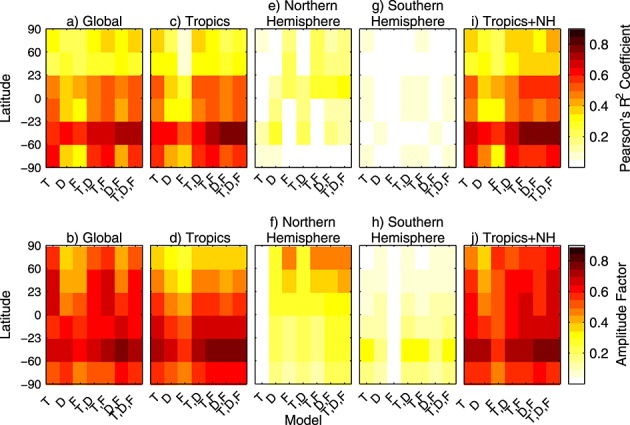
Goodness-of-fit metrics for models of increasing complexity. (top) The Pearson's R² coefficient (an indication of correlation between observed and simulated CO₂ variability) and (bottom) the relative amplitude factor (equation (4)) as the goodness-of-fit metric. The value of each metric is shown for (a and b) global fluxes, (c and d) tropical fluxes, (e and f) Northern Hemisphere fluxes, (g and h) Southern Hemisphere fluxes, and (i and j) linear combinations of both tropical and Northern Hemisphere fluxes. For each panel, T represents an NEE model driven solely by temperature, D an NEE model driven solely by PDSI, and F a model driven solely by GFED fire emissions. Other models are a combination of these individual drivers. The relative amplitude is the standard deviation of the simulated CO₂ from the model divided by the standard deviation of observed CO₂ and is an indication of the magnitude of variability contributed by each flux model.

We developed several regression models combining temperature, drought stress, and fire components. For this analysis, we used PDSI-driven NEE and GFED3 fire emissions since these single-factor regressions performed better than other models within the same class (Table 2), and we focused on fluxes originating in the tropics and Northern Hemisphere. In general, these models were able to explain more of the CO₂ variability in the Southern Hemisphere than in the Northern Hemisphere, in part due to greater high frequency variability in Northern Hemisphere observations (Figures 1 and 4). Given significant correlations among various drivers (e.g., Figure 3), the scale factors (λ) for the multidriver regression models had reduced magnitudes compared to the corresponding single-driver regressions since the signal amplitude was spread across multiple drivers (Table 5).

Table 5.

Optimal Coefficients (λ) From Each Component in Multidriver Regression Models^a

Regression Model	Global mean R2	Tropical T	Tropical PDSI	Tropical GFED	Northern Hemisphere T	Northern Hemisphere PDSI	Northern Hemisphere GFED
Tropical T	0.48	0.67 ± 0.06
Tropical (T, D)	0.49	0.69 ± 0.14	0.02 ± 0.11
Tropical (T, F)	0.51	0.54 ± 0.07		0.14 ± 0.04
Tropical (D, F)	0.48		−0.36 ± 0.05	0.22 ± 0.04
Tropical (T, D, F)	0.52	0.45 ± 0.14	−0.07 ± 0.10	0.15 ± 0.04
NH (T, D)	0.12				0.10 ± 0.11	0.27 ± 0.11
NH (T, F)	0.13				0.03 ± 0.09		0.20 ± 0.06
NH (D, F)	0.16					0.18 ± 0.09	0.17 ± 0.07
NH (T, D, F)	0.17				0.10 ± 0.10	0.21 ± 0.10	0.17 ± 0.06
Best case	0.56	0.43 ± 0.12	−0.16 ± 0.10	0.17 ± 0.04	0.06 ± 0.06	−0.17 ± 0.06	0.13 ± 0.04

^aThe best case model includes six driver variables: temperature, PDSI, and GFED3 contributions in both the tropics and NH.

For a best-case model estimate, we optimized λ coefficients for temperature, drought, and fires from the Northern Hemisphere and tropics simultaneously. This model, comprised of six basis functions, explained 39 to 57% of the observed variability in the Northern Hemisphere and 52 to 79% of the variability in the Southern Hemisphere (Figure 5). The combined contributions from fires and NEE responses to drought stress accounted for 60–70% of the model variability in each latitude belt (Figure 6a). The direct temperature response of NEE contributed between 30–37% of model variability in the Northern Hemisphere and 39–40% in the Southern Hemisphere. Thus, although direct control of NEE by temperature was the single largest driver of observed variability in atmospheric CO₂ (except north of 23°N), the contribution from temperature was smaller than the sum of drought and fire components, contrasting with results reported by [Wang et al., ²⁰¹³]. We tested an alternative version of the best-case model, substituting precipitation for PDSI as the climate proxy for drought stress, and regression results indicated a further reduction in the contribution from tropical temperature to CO₂ variability (Figure 6b).

Figure 5.

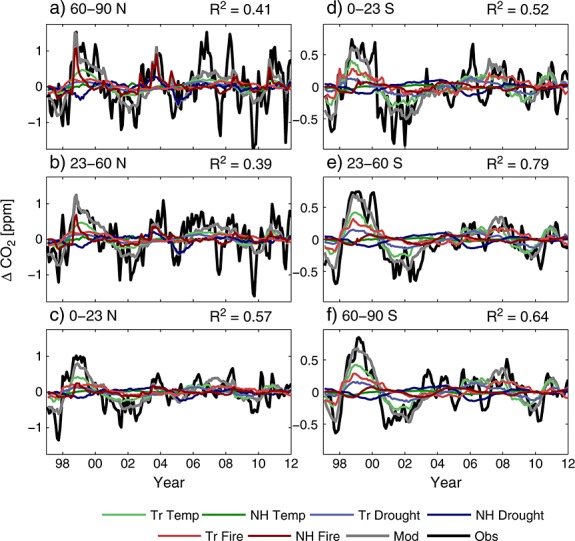
Contributions of tropical (Tr) and Northern Hemisphere (NH) temperature, drought stress (PDSI), and fire emissions (GFED3) to atmospheric CO₂ interannual variability by latitude. The Pearson's R² coefficient for each latitude band is given in the upper right hand corner. The best-case model (Mod) is shown with a grey line and the observations (Obs) with a black line. The black lines denoting the observations were not identical to the time series shown in Figure 1 because a refinement to the third-order detrending polynomial was fit based on the residual between the observations and the optimized model. Note also the change in y axis scale between the Northern and Southern Hemispheres.

Figure 6.

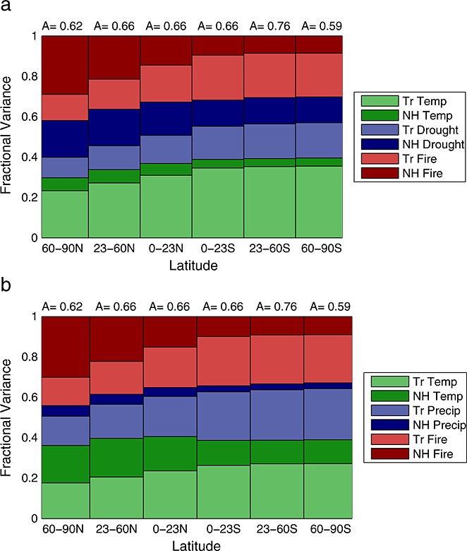
(a) Relative contributions to the simulated variability in atmospheric CO₂ in different latitude bands (x axis) from NEE responses to temperature and drought stress (PDSI), and fire emissions (GFED3) originating from the tropics and Northern Hemisphere. The amplitude factor (A), calculated as the ratio of the standard deviation of the simulated CO₂ relative to the standard deviation of the observations, is shown for each latitudinal band. (b) Using GPCP precipitation rather than PDSI as a drought stress metric further diminishes the contribution of tropical temperature to interannual variability in atmospheric CO₂.

Simultaneously accounting for temperature, drought, and fire in the best-case model improved both goodness-of-fit metrics compared to models that assumed only a single driver (Figures 5 and 6, and Table 2). Accounting for correlations among successive monthly observations, the calculated F statistic justified the additional degrees of freedom in the best-case model relative to the tropical temperature-only model (p < 0.01). Moreover, synthetic data generated from the best-case model, as opposed to those from the tropical temperature-only model, were more consistent with the atmospheric observations (Figure 7). One rationale that has been given for using the present-day temperature sensitivity of the CO₂ growth rate as a constraint on future model projections is that the apparent temperature sensitivity implicitly captures the covarying sensitivity to drought and fire; if that were the case, synthetic CO₂ generated from a tropical temperature-only regression model should yield the same sensitivity to drought and fire as atmospheric observations. However, when the synthetic temperature data were fit serially using single-driver, single-region regression models, the λ values were significantly different from those determined from atmospheric observations, ruling out the possibility that a tropical temperature-only model is sufficient to describe the observations.

Figure 7.

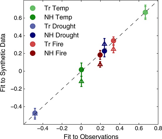
Scale factors for single drivers when fit to observations versus when fit to synthetic data derived from tropical temperature-only and best-case regression models. We generated 1000 realizations of synthetic CO₂ using parameter values drawn from the uncertainty distributions of the tropical temperature-only and the best-case regression models, and fit single-driver temperature, drought, and fire response functions to the synthetic data. The individual λ values fit to the synthetic data derived from the best-case model (circles) were consistent with those fit to the observations, while the Northern Hemisphere λ values and tropical fire λ value fit to the temperature-only synthetic data deviated significantly (triangles), ruling out the possibility that the tropical temperature-only model was consistent with the observations (p < 10⁻³).

Fire contributions to CO₂ variability in the best-case model varied with latitude. Fires had a greater impact in the Northern Hemisphere (33–42%) than in the Southern Hemisphere (30–32%), where fire emissions from boreal forests were large relative to other surface fluxes. In the Northern Hemisphere, the standard deviation of the fire flux in the best-case model increased to 0.13 ± 0.04 Pg C yr⁻¹ from the GFED3 baseline of 0.10 Pg C yr⁻¹. In contrast, the standard deviation of the optimized tropical fire emissions was significantly lower than the standard deviation within the tropics from GFED3 (0.17 ± 0.04 Pg C yr⁻¹ versus 0.30 Pg C yr⁻¹).

The ability to isolate the contributions from temperature, drought, and fire in the meridional distribution of CO₂ was lost when these data were aggregated to a global, area-weighted CO₂ time series. For the best-case model described above, the tropical fire contribution decreased by 60% when fit against a globally averaged CO₂ timeseries rather than against the meridional structure of CO₂ (Table 6). In contrast, the optimal flux magnitude for Northern Hemisphere fire emissions increased several fold (Table 6)—an unrealistic increase given available constraints from CH₄ and CO. When we averaged the global mean CO₂ data to annual time steps, the tropical fire emissions component was further reduced. These exercises demonstrated that aggregating CO₂ data over larger spatial scales and longer time scales may mask contributions from fire emissions observed at higher resolutions.

Table 6.

Optimal Scale Factors (λ) and Globally Averaged Amplitude Factors (A) for Tropical or Northern Hemisphere GFED Fire Emissions Based on Spatial and Temporal Averaging of Monthly Atmospheric CO₂ Data

	Regional Averaging		Global Averaging		Global, Yearly Averaging
Model Case	λFire	A	λFire	A	λFire	A
Tropical (T, F)	0.14	0.28	0.06	0.13	0.07	0.14
Tropical (D, F)	0.22	0.42	0.18	0.35	0.18	0.38
Tropical (T, D, F)	0.15	0.29	0.05	0.07	0.03	0.03
Northern (T, F)	0.20	0.90	0.40	0.73	0.69	0.74
Northern (D, F)	0.17	0.53	0.39	0.77	0.64	0.77
Northern (T, D, F)	0.17	0.41	0.35	0.41	0.62	0.42
Bestcase, tropical F	0.17	0.19	0.06	0.06	0.00	0.00

Estimates of the temperature or drought sensitivity of NEE at large temporal and spatial scales are required for ecosystem model evaluation. Specifically, atmospheric CO₂ responses to regionally coherent climate anomalies provide an opportunity to quantify biome-level responses that integrate across regional variations in species composition, moisture availability, and other important drivers of ecosystem processes that are difficult to represent in global models. This information is complementary to canopy-scale responses derived from eddy covariance observations [e.g., Schwalm et al., ²⁰¹⁰]. We determined the large-scale sensitivity of NEE to temperature and drought stress by regressing the land area-weighted monthly NEE fluxes derived from our optimized models against the land area-weighted average of monthly temperature or PDSI anomalies (Figure 8). Accounting for fire emissions considerably reduced the sensitivity of NEE to temperature and drought stress inferred from the atmospheric CO₂ observations (Table 7). We found that the temperature sensitivity of tropical NEE was 3.9 ± 0.4 Pg C yr⁻¹ K⁻¹ when no other climate drivers or fire fluxes were taken into consideration. When we applied the λ value from a model that included global fire emissions, the temperature sensitivity of tropical NEE decreased by 25% to 2.9 ± 0.4 Pg C yr⁻¹ K⁻¹. The sensitivity of tropical NEE to temperature was further reduced to 2.6 ± 0.7 Pg C yr⁻¹ K⁻¹ when we considered all scale factors from the best-case model (Figure 9). The NEE sensitivity to tropical drought stress likewise decreased by 30%, from −1.1 ± 0.1 Pg C yr⁻¹ per unit of PDSI when no other drivers were considered to −0.8 ± 0.1 Pg C yr⁻¹ per unit of PDSI when we accounted for global fire emissions (Table 7).

Figure 8.

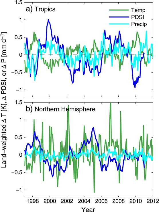
Land-weighted temperature, precipitation, and PDSI anomalies for the tropics and Northern Hemisphere.

Table 7.

Sensitivity of NEE to Temperature and Drought Stress (Normalized to a 1 Unit Increase in the Palmer Drought Severity Index) When NEE Responses Were Considered Alone or in Conjunction With Fire Emissions^a

Flux	Original	Accounting for Fire	Significance of F Test
NEE Sensitivity to Temperature (Pg C yr−1 K−1)
Tropical NEE	3.9 ± 0.4	2.9 ± 0.4	p < 0.01
Global NEE	3.3 ± 0.3	2.4 ± 0.3	p < 0.01
NEE Sensitivity to Drought (PDSI) (Pg C yr−1 per unit of PDSI)
Tropical NEE	−1.1 ± 0.1	−0.8 ± 0.1	p < 0.001
Global NEE	−1.6 ± 0.2	−1.1 ± 0.2	p < 0.001

^aAn F test was used to compare model pairs with and without fire.

Figure 9.

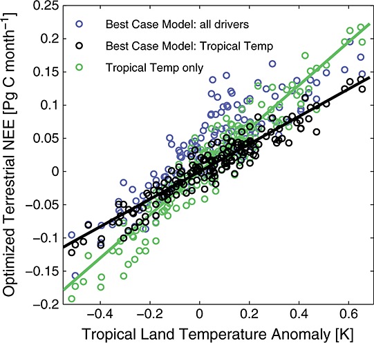
Optimized terrestrial ecosystem flux anomalies for two model cases. The best-case model (blue) represents the sum of fluxes from temperature-driven NEE, PDSI-driven NEE, and fire-driven NEE in the tropics and Northern Hemisphere. Its tropical temperature component has been plotted separately (black). The tropical temperature case (green) only includes temperature-driven fluxes in the tropics.

4 Discussion

Our results suggest that the correlation between tropical temperature and the CO₂ growth rate is caused by an assortment of covarying processes, including NEE responses to temperature and drought stress as well as fire emissions in tropical and boreal forest ecosystems. We found that the combined influence of the response of NEE to drought and fire emissions accounted for more of the variability than direct temperature responses of NEE when these drivers were considered simultaneously. These findings have several implications for studies that use contemporary CO₂ variability to constrain ESMs.

First, fire, temperature, and drought responses within ESMs need to be separately and explicitly considered during model evaluation. Cox et al. [2013] developed a novel approach for constraining the long-term sensitivity of tropical carbon stocks to warming (γ) in ESMs using contemporary atmospheric CO₂ and temperature observations. The authors showed that a relationship existed across different models between γ and the interannual CO₂ growth rate sensitivity to temperature. In a second step, Cox et al. used observations from the past several decades to show that many models overestimated the observed CO₂ growth rate sensitivity to temperature and thus had γ values that were likely excessive. Several models, however, were near or within the range of the observations. Since many of the models in the ensemble did not have explicit representation of fire processes, removing fire contributions from the observed CO₂ growth rate may enable a more direct comparison with simulated NEE responses to tropical temperature. Our results suggest that after removing fire contributions, the component of the observed CO₂ growth rate variability attributable to tropical NEE would be reduced by approximately 25% (e.g., Table 7), bringing a different set of models into closer agreement with the observed range. Although a more rigorous evaluation is needed, this preliminary estimate strengthens conclusions by Cox et al. that earlier models may have had unrealistically large (negative) values of γ—at least for the nonfire component of the tropical net ecosystem carbon balance. It is important to recognize that while ESM agreement with present-day CO₂ variability and its multiple drivers is necessary to have confidence in climate predictions, it is not sufficient because, on longer time scales, climate changes would be expected to modify processes that are likely of second-order importance to the interannual variations we analyze here, including plant competition and tree mortality.

Second, estimates of the fire contribution to CO₂ variability change significantly with temporal and spatial averaging. The standard deviation of optimized tropical fire emissions decreased by 60–70% when CO₂ variability was averaged globally and by up to 80% when variability was determined from annual, rather than monthly, CO₂ time series. This result underscores the need to consider the full spatial and temporal distribution of atmospheric CO₂ and to use a consistent transport-modeling framework to infer the sensitivities to temperature and drought stress in both models and observations. The extension of column CO₂ time series from GOSAT and forthcoming observations from NASA's Orbiting Carbon Observatory (OCO-2, launched in 2014) may enable future refinements in the partitioning among temperature, drought, and fire contributions to CO₂ variability.

Fire management is one possible lever for reducing CO₂ emissions as the climate warms. In the tropics, where fires are often linked with forest and peatland clearing, different management practices may lead to greater long-term carbon storage. Optimizing long-term development strategies [Nepstad et al., ¹⁹⁹⁹] or more effective use of fire forecasting tools [Chen et al., ²⁰¹¹], for example, may ultimately enable managers to reduce carbon losses. Accurate attribution of interannual variability of CO₂ to fire and NEE responses to drought and temperature also may improve our understanding of drivers of long-term changes in this variability [Wang et al., ²⁰¹⁴] and reveal opportunities for decoupling carbon fluxes from drought stress as climate changes.

Analysis of the climate drivers of CO₂ variability at seasonal, interannual, and decadal time scales may ultimately provide a path toward improved climate predictability in ESMs. We stress that capturing variability at these time scales does not ensure accurate climate predictions at longer time scales, but only improves our confidence that important mechanisms are adequately represented. The linkages among temperature, drought, and fire contributions in this study underscore their similar responses to climate variability and the importance of balanced investments in field and modeling research programs that improve our understanding of all of these interactions and their representation in ESMs.

References

- Adler RF, et al. The Version-2 Global Precipitation Climatology Project (GPCP) monthly precipitation analysis (1979–present) J. Hydrometeorol. 2003;4(6):1147–1167. doi: 10.1175/1525-7541(2003)004<1147:TVGPCP>2.0.CO;2. [Google Scholar]
- Akagi SK, Yokelson RJ, Wiedinmyer C, Alvarado MJ, Reid JS, Karl T, Crounse JD. Wennberg PO. Emission factors for open and domestic biomass burning for use in atmospheric models. Atmos. Chem. Phys. 2011;11(9):4039–4072. doi: 10.5194/acp-11-4039-2011. [Google Scholar]
- Alden CB, Miller JB. White JWC. Can bottom-up ocean CO2 fluxes be reconciled with atmospheric 13C observations? Tellus B. 2010;62(5):369–388. doi: 10.1111/j.1600-0889.2010.00481.x. [Google Scholar]
- Andreae MO. Merlet P. Emission of trace gases and aerosols from biomass burning. Global Biogeochem. Cycles. 2001;15(4):955–966. doi: 10.1029/2000GB001382. [Google Scholar]
- Andres RJ, Gregg JS, Losey L, Marland G. Boden TA. Monthly, global emissions of carbon dioxide from fossil fuel consumption. Tellus B. 2011;63(3):309–327. doi: 10.1111/j.1600-0889.2011.00530.x. [Google Scholar]
- Arino O. Melinotte JM. The 1993 Africa fire map. Int. J. Remote Sens. 1998;19(11):2019–2023. doi: 10.1080/014311698214839. [Google Scholar]
- Atkin O. Thermal acclimation and the dynamic response of plant respiration to temperature. Trends Plant Sci. 2003;8(7):343–351. doi: 10.1016/S1360-1385(03)00136-5. doi: 10.1016/s1360-1385(03)00136-5. [DOI] [PubMed] [Google Scholar]
- Bacastow RB. Modulation of atmospheric carbon dioxide by the Southern Oscillation. Nature. 1976;261:116–118. [Google Scholar]
- Battle MO, Bender ML, Tans PP, White JW, Ellis JT, Conway TJ. Francey RJ. Global carbon sinks and their variability inferred from atmospheric O2 and δ13C. Science. 2000;287(287):2467–2470. doi: 10.1126/science.287.5462.2467. [DOI] [PubMed] [Google Scholar]
- Berry J. Bjorkman O. Photosynthetic response and adaptation to temperature in higher plants. Annu. Rev. Plant Physiol. 1980;31(1):491–543. doi: 10.1146/annurev.pp.31.060180.002423. [Google Scholar]
- Bonal D, et al. Impact of severe dry season on net ecosystem exchange in the neotropical rainforest of French Guiana. Global Change Biol. 2008;14(8):1917–1933. doi: 10.1111/j.1365-2486.2008.01610.x. [Google Scholar]
- Bousquet P, Peylin P, Ciais P, Le Quéré C, Friedlingstein P. Tans PP. Regional changes in carbon dioxide fluxes of land and oceans since 1980. Science. 2000;290(5495):1342–1346. doi: 10.1126/science.290.5495.1342. [DOI] [PubMed] [Google Scholar]
- Bousquet P, et al. Contribution of anthropogenic and natural sources to atmospheric methane variability. Nature. 2006;443(7110):439–443. doi: 10.1038/nature05132. doi: 10.1038/nature05132. [DOI] [PubMed] [Google Scholar]
- Bowman DM, et al. The human dimension of fire regimes on Earth. J. Biogeogr. 2011;38(12):2223–2236. doi: 10.1111/j.1365-2699.2011.02595.x. doi: 10.1111/j.1365-2699.2011.02595.x. [DOI] [PMC free article] [PubMed] [Google Scholar]
- Braswell BH. The response of global terrestrial ecosystems to interannual temperature variability. Science. 1997;278(5339):870–873. doi: 10.1126/science.278.5339.870. [Google Scholar]
- Chen Y, Randerson JT, Morton DC, DeFries RS, Collatz GJ, Kasibhatla PS, Giglio L, Jin Y. Marlier ME. Forecasting fire season severity in South America using sea surface temperature anomalies. Science. 2011;334(6057):787–791. doi: 10.1126/science.1209472. doi: 10.1126/science.1209472. [DOI] [PubMed] [Google Scholar]
- Cox PM, Pearson D, Booth BB, Friedlingstein P, Huntingford C, Jones CD. Luke CM. Sensitivity of tropical carbon to climate change constrained by carbon dioxide variability. Nature. 2013;494(7437):341–344. doi: 10.1038/nature11882. doi: 10.1038/nature11882. [DOI] [PubMed] [Google Scholar]
- Dai A, Trenberth KE. Qian TT. A global dataset of Palmer Drought Severity Index for 1870–2002: Relationship with soil moisture and effects of surface warming. J. Hydrometeorol. 2004;5:1117–1130. [Google Scholar]
- Davidson EA. Janssens IA. Temperature sensitivity of soil carbon decomposition and feedbacks to climate change. Nature. 2006;440(7081):165–173. doi: 10.1038/nature04514. doi: 10.1038/nature04514. [DOI] [PubMed] [Google Scholar]
- Dlugokencky EJ, Lang PM, Masarie K, Crotwell AM. Crotwell MJ. 2013. and Atmospheric carbon dioxide dry air mole fractions from the NOAA ESRL carbon cycle cooperative global air sampling network, 1968–2012.
- Doney SC, Lima I, Feely RA, Glover DM, Lindsay K, Mahowald N, Moore JK. Wanninkhof R. Mechanisms governing interannual variability in upper-ocean inorganic carbon system and air–sea CO2 fluxes: Physical climate and atmospheric dust. Deep Sea Res., Part II. 2009;56(8–10):640–655. doi: 10.1016/j.dsr2.2008.12.006. [Google Scholar]
- Doughty CE. Goulden ML. Are tropical forests near a high temperature threshold? J. Geophys. Res. 2008;113 G00B07, doi: 10.1029/2007JG000632. [Google Scholar]
- Farquhar GD. Roderick ML. Pinatubo, diffuse light, and the carbon cycle. Science. 2003;299(5615):1997–1998. doi: 10.1126/science.1080681. doi: 10.1126/science.1080681. [DOI] [PubMed] [Google Scholar]
- Francey RJ, Tans PP, Allison CE, Enting IG, White JWC. Trolier M. Changes in oceanic and terrestrial carbon uptake since 1982. Nature. 1995;373(6512):326–330. [Google Scholar]
- Frölicher TL, Joos F, Raible CC. Sarmiento JL. Atmospheric CO2 response to volcanic eruptions: The role of ENSO, season, and variability. Global Biogeochem. Cycles. 2013;27:239–251. doi: 10.1002/gbc.20028. [Google Scholar]
- Gatti LV, et al. Drought sensitivity of Amazonian carbon balance revealed by atmospheric measurements. Nature. 2014;506(7486):76–80. doi: 10.1038/nature12957. doi: 10.1038/nature12957. [DOI] [PubMed] [Google Scholar]
- Gelman A, Li Meng X. Stern H. Posterior predictive assessment of model fitness via realized discrepancies. Statistica Sinica. 1996;6:733–807. [Google Scholar]
- Jones CD, Collins M, Cox PM. Spall SA. The carbon cycle response to ENSO: A coupled climate–carbon cycle model study. J. Clim. 2001;14(21):4113–4129. doi: 10.1175/1520-0442(2001)014<4113:TCCRTE>2.0.CO;2. [Google Scholar]
- Jones PD, Lister DH, Osborn TJ, Harpham C, Salmon M. Morice CP. Hemispheric and large-scale land-surface air temperature variations: An extensive revision and an update to 2010. J. Geophys. Res. 2012;117 D05127, doi: 10.1029/2011JD017139. [Google Scholar]
- Kalnay E, et al. The NCEP/NCAR 40-year reanalysis project. Bull. Am. Meteorol. Soc. 1996;77(3):437–471. doi: 10.1175/1520-0477(1996)077<0437:TNYRP>2.0.CO;2. [Google Scholar]
- Kasischke ES, Hyer EJ, Novelli PC, Bruhwiler LP, French NHF, Sukhinin AI, Hewson JH. Stocks BJ. Influences of boreal fire emissions on Northern Hemisphere atmospheric carbon and carbon monoxide. Global Biogeochem. Cycles. 2005;19 GB1012, doi: 10.1029/2004GB002300. [Google Scholar]
- Keeling CD, Whorf TP, Wahlen M. Vanderplicht J. Interannual extremes in the rate of rise of atmospheric carbon dioxide since 1980. Nature. 1995;375:666–670. [Google Scholar]
- Keppel-Aleks G, et al. Atmospheric carbon dioxide variability in the Community Earth System Model: Evaluation and transient dynamics during the twentieth and twenty-first centuries. J. Clim. 2013;26(13):4447–4475. doi: 10.1175/jcli-d-12-00589.1. [Google Scholar]
- Langenfelds RL, Francey RJ, Pak BC, Steele LP, Lloyd J, Trudinger CM. Allison CE. Interannual growth rate variations of atmospheric CO2 and its δ13C, H2, CH4, and CO between 1992 and 1999 linked to biomass burning. Global Biogeochem. Cycles. 2002;16(3) and ), 1048, doi: 10.1029/2001GB001466. [Google Scholar]
- Mahecha MD, et al. Global convergence in the temperature sensitivity of respiration at ecosystem level. Science. 2010;329(5993):838–840. doi: 10.1126/science.1189587. doi: 10.1126/science.1189587. [DOI] [PubMed] [Google Scholar]
- Nassar R, et al. Modeling global atmospheric CO2 with improved emission inventories and CO2 production from the oxidation of other carbon species. Geosci. Model Dev. 2010;3(2):689–716. doi: 10.5194/gmd-3-689-2010. [Google Scholar]
- Nepstad DC, et al. Large-scale impoverishment of Amazonian forests by logging and fire. Nature. 1999;398(6727):505–508. [Google Scholar]
- Nevison CD, Mahowald NM, Doney SC, Lima ID, van der Werf GR, Randerson JT, Baker DF, Kasibhatla P. McKinley GA. Contribution of ocean, fossil fuel, land biosphere, and biomass burning carbon fluxes to seasonal and interannual variability in atmospheric CO2. J. Geophys. Res. 2008;113 G01010, doi: 10.1029/2007JG000408. [Google Scholar]
- Nobre P. Shukla J. Variations of sea surface temperature, wind stress, and rainfall over the tropical Atlantic and South America. J. Clim. 1996;9(10):2464–2479. doi: 10.1175/1520-0442(1996)009<2464:VOSSTW>2.0.CO;2. [Google Scholar]
- Plumb RA. Mahlman JD. The zonally averaged transport characteristics of the GFDL general circulation/transport model. J. Atmos. Sci. 1987;44(2):298–327. doi: 10.1175/1520-0469(1987)044<0298:TZATCO>2.0.CO;2. [Google Scholar]
- Rafelski LE, Piper SC. Keeling RF. Climate effects on atmospheric carbon dioxide over the last century. Tellus B. 2009;61(5):718–731. doi: 10.1111/j.1600-0889.2009.00439.x. [Google Scholar]
- Randerson JT, Thompson MV, Conway TJ, Fung I. Field CB. The contribution of terrestrial sources and sinks to trends in the seasonal cycle of atmospheric carbon dioxide. Global Biogeochem. Cycles. 1997;11(4):535–560. doi: 10.1029/97GB02268. [Google Scholar]
- Randerson JT, van der Werf GR, Collatz GJ, Giglio L, Still CJ, Kasibhatla P, Miller JB, White JWC, DeFries RS. Kasischke ES. Fire emissions from C3 and C4 vegetation and their influence on interannual variability of atmospheric CO2 and δ13CO2. Global Biogeochem. Cycles. 2005;19 GB2019, doi: 10.1029/2004GB002366. [Google Scholar]
- Rayner PJ, Law RM, Allison CE, Francey RJ, Trudinger CM. Pickett-Heaps C. Interannual variability of the global carbon cycle (1992–2005) inferred by inversion of atmospheric CO2 and δ13CO2 measurements. Global Biogeochem. Cycles. 2008;22 GB3008, doi: 10.1029/2007GB003068. [Google Scholar]
- Reichstein M, et al. Climate extremes and the carbon cycle. Nature. 2013;500(7462):287–295. doi: 10.1038/nature12350. doi: 10.1038/nature12350. [DOI] [PubMed] [Google Scholar]
- Rienecker MM, et al. MERRA: NASA's modern-era retrospective analysis for research and applications. J. Clim. 2011;24(14):3624–3648. doi: 10.1175/JCLI-D-16-0758.1. doi: 10.1175/jcli-d-11-00015.1. [DOI] [PMC free article] [PubMed] [Google Scholar]
- Ropelewski CF. Halpert MS. Global and regional scale precipitation patterns associated with the El Niño/Southern Oscillation. Mon. Weather Rev. 1987;115(8):1606–1626. doi: 10.1175/1520-0493(1987)115<1606:GARSPP>2.0.CO;2. [Google Scholar]
- Saleska SR, et al. Carbon in Amazon forests: Unexpected seasonal fluxes and disturbance-induced losses. Science. 2003;302(5650):1554–1557. doi: 10.1126/science.1091165. doi: 10.1126/science.1091165. [DOI] [PubMed] [Google Scholar]
- Schwalm CR, et al. Assimilation exceeds respiration sensitivity to drought: A FLUXNET synthesis. Global Change Biol. 2010;16(2):657–670. doi: 10.1111/j.1365-2486.2009.01991.x. [Google Scholar]
- Schwalm CR, Williams CA, Schaefer K, Baker I, Collatz GJ. Rödenbeck C. Does terrestrial drought explain global CO2 flux anomalies induced by El Niño? Biogeosciences. 2011;8(9):2493–2506. doi: 10.5194/bg-8-2493-2011. [Google Scholar]
- Suntharalingam P, Jacob DJ, Palmer PI, Logan JA, Yantosca RM, Xiao Y. Evans MJ. Improved quantification of Chinese carbon fluxes using CO2/CO correlations in Asian outflow. J. Geophys. Res. 2004;109 D18S18, doi: 10.1029/2003JD004362. [Google Scholar]
- Todd-Brown KEO, Randerson JT, Post WM, Hoffman FM, Tarnocai C, Schuur EAG. Allison SD. Causes of variation in soil carbon simulations from CMIP5 Earth system models and comparison with observations. Biogeosciences. 2013;10(3):1717–1736. doi: 10.5194/bg-10-1717-2013. [Google Scholar]
- van der Werf GR, Randerson JT, Collatz GJ, Giglio L, Kasibhatla PS, Arellano AF, Jr, Olsen SC. Kasischke ES. Continental-scale partitioning of fire emissions during the 1997 to 2001 El Nino/La Nina period. Science. 2004;303(5654):73–76. doi: 10.1126/science.1090753. doi: 10.1126/science.1090753. [DOI] [PubMed] [Google Scholar]
- van der Werf GR, Randerson JT, Giglio L, Collatz GJ, Mu M, Kasibhatla PS, Morton DC, DeFries RS, Jin Y. van Leeuwen TT. Global fire emissions and the contribution of deforestation, savanna, forest, agricultural, and peat fires (1997–2009) Atmos. Chem. Phys. 2010;10(23):11,707–11,735. doi: 10.5194/acp-10-11707-2010. [Google Scholar]
- Wang W, Ciais P, Nemani RR, Canadell JG, Piao S, Sitch S, White MA, Hashimoto H, Milesi C. Myneni RB. Variations in atmospheric CO2 growth rates coupled with tropical temperature. Proc. Natl. Acad. Sci. U.S.A. 2013;110(32):13,061–13,066. doi: 10.1073/pnas.1219683110. doi: 10.1073/pnas.1219683110. [DOI] [PMC free article] [PubMed] [Google Scholar]
- Wang X, et al. A two-fold increase of carbon cycle sensitivity to tropical temperature variations. Nature. 2014;506(7487):212–215. doi: 10.1038/nature12915. doi: 10.1038/nature12915. [DOI] [PubMed] [Google Scholar]
- Zeng F-W, Collatz G, Pinzon J. Ivanoff A. Evaluating and quantifying the climate-driven interannual variability in Global Inventory Modeling and Mapping Studies (GIMMS) Normalized Difference Vegetation Index (NDVI3g) at global scales. Remote Sens. 2013;5(8):3918–3950. [Google Scholar]
- Zeng N, Mariotti A. Wetzel P. Terrestrial mechanisms of interannual CO2 variability. Global Biogeochem. Cycles. 2005;19 GB1016, doi: 10.1029/2004GB002273. [Google Scholar]