Optimization of Large-scale Mouse Brain Connectome via Joint Evaluation of DTI and Neuron Tracing Data

Abstract

Tractography based on Diffusion tensor imaging (DTI) data has been used as a tool by a large number of recent studies to investigate structural connectome. Despite its great success in offering unique 3D neuroanatomy information, DTI is an indirect observation with limited resolution and accuracy and its reliability is still unclear. Thus, it is essential to answer this fundamental question: how reliable is DTI tractography in constructing large-scale connectome? To answer this question, we employed neuron tracing data of 1772 experiments in the mouse brain released by the Allen Mouse Brain Connectivity Atlas (AMCA) as the ground-truth to assess the performance of DTI tractography in inferring white matter fiber pathways and inter-regional connections. For the first time in the neuroimaging field, the performance of whole brain DTI tractography in constructing large-scale connectome has been evaluated by comparison with tracing data. Our results suggested that only with the optimized tractography parameters and the appropriate scale of brain parcellation scheme, DTI can produce relatively reliable fiber pathways and large-scale connectome. Meanwhile, a considerable amount of errors were also identified in optimized DTI tractography results, which we believe could be potentially alleviated by effort in developing better DTI tractography approaches. In this scenario, our framework could serve as a reliable and quantitative test bed to identify errors in tractography results which will facilitate the development of such novel tractography algorithms and the selection of optimal parameters.

Graphical abstract

1 Introduction

Mapping brain activity patterns and deciphering neural codes are the fundamental goals of the BRAIN project (http://www.nih.gov/science/brain/) (NIH, 2014; Tsien et al., 2013). The achievement of the goal requires a comprehensive view of the structural connectivity patterns from which neural activity patterns are generated. Since the early development of diffusion tensor imaging (DTI) (Basser et al., 1994) and tractography algorithms (Mori et al., 1999) in 1990s, the technique has been widely applied to investigate white matter pathways of mammalian brains. As a magnetic resonance imaging (MRI) technique, DTI is able to infer axonal fiber orientations of living brains in 3D space by measuring restricted water diffusion in tissue. Based on the DTI tractography, many macro-scale fiber pathways of mammalian brains such as human (Assaf and Pasternak, 2008; Bassett and Bullmore, 2009; Mori et al., 2008), macaque (Chen et al., 2013; Li et al., 2013; Rilling et al., 2008), or mouse (Calamante et al., 2012; Moldrich et al., 2010; Zhang et al., 2002) were reconstructed and analyzed. Later, it has been pointed out that in order to fully understand how the brain works, a comprehensive map of brain inter-regional wiring diagram on a large scale, namely connectome, is required (Bullmore and Sporns, 2009; Sporns et al., 2005; Van Essen, 2013). Moreover, several more advanced diffusion MRI approaches such as high angular resolution diffusion imaging (HARDI) (Tuch et al., 2002) or diffusion spectrum imaging (DSI) (Wedeen et al., 2005) were developed to overcome the limitation of DTI in reconstructing crossing fibers. As the only feasible neuroimaging approach to investigate structural connectome in living brain, DTI tractography as well as its advanced form has been used as a presumably reliable tool by a large number of large-scale studies. For example, the Human Connectome Project (Sotiropoulos et al., 2013; Van Essen et al., 2012) (http://www.humanconnectome.org/) is acquiring HARDI data of 1200 healthy subjects to build a connection map of brain; the CONNECT project (Assaf et al., 2013) has been developing tools to analyze the brain’s macro- and micro-structure tissues and connectivities by combining tractography and micro-structural measurement in diffusion MRI data; the Brainnetome Project (Jiang, 2014, 2013) (http://www.brainnetome.org) is comparing DTI data of thousands of patients and the healthy controls to explore the brain’s network-based biomarkers for brain diseases such as schizophrenia and Alzheimer’s disease; the Brain Decoding Project (http://braindecodingproject.org/) is analyzing mouse brain data on different scales with different imaging modalities including DTI to unveil the myth of memory.

In spite of the growing exciting findings brought by DTI, the reliability of DTI-based tractography is still in question. DTI showed a variety of limitations, especially when it is applied to infer inter-regional connections. In the review article by Jbabdi and Johansen-Berg, DTI tractography is regarded as an “indirect, inaccurate, and difficult to quantify” observation approach (Jbabdi and Johansen-Berg, 2011). Different from the traditional histology approach which directly observes neurons and axons under microscope, DTI infers microanatomy indirectly from properties of restricted water diffusion in tissue, resulting in the loss of information on the microscale structures. For example, as reviewed in (Jbabdi and Johansen-Berg, 2011), it is difficult to determine where a fiber tract should start or terminate. Long association tracts constructed by DTI tractography could be a long direct connection between remote cortical regions, or, alternatively, a succession of short fibers. Moreover, DTI tractography is unable to identify the polarity of a given connection. An afferent axon cannot be distinguished from an efferent axon based on their water diffusion pattern. Though one could argue that the detailed information like synapse structure or polarity is not necessary for analysis on a macro-scale. The accuracy of the approach is still questionable for such kind of analysis due to the empirical models and parameters applied to axonal fiber tractography. The classic DTI tractography methodology assumes that axonal fiber bundles move in parallel in a single voxel and thus models each voxel with single diffusion model. However, the assumptions can only be met if the resolution is high enough to monitor a single bundle of axons. In reality, a voxel typically contains tens of thousands axons from different bundles. In addition to traveling in parallel, they could meet, merge, twist, bend, cross, etc. Therefore, a voxel cannot be modeled by a single diffusion model. Notably, some of the axon interactions such as crossing or diverging have been modeled by advanced tractography methods (Hess et al., 2006; Wedeen et al., 2008; Zhang et al., 2012). But due to a lack of the ground truth or alternative validation methods, the accuracy of the models remains untested, and the models and parameters applied by those approaches are highly empirical. Further, even with the most accurate model and optimal parameters have been applied, findings are still quite sensitive to the selection of brain parcellation scheme (Meskaldji et al., 2013; Zalesky et al., 2010). Given the limited resolution of DTI data, it is not clear on which scale (volume size of regions of interest) tractography gives the best performance. With all these limitations raised above and a large number of ongoing brain connectome-related studies based on DTI tractography, we believe that it is essential to reexamine the basic question: How reliable is large-scale connectome constructed by DTI?

So far, the most ideal approach to validate DTI tractography is neuron tracing study. The merit of this approach is that it allows accurate observations of inter-regional connections and white matter fiber pathways in the brain of the sacrificed animal. Different from the dye applied in traditional histology study that target on specific tissue/molecule, neuron tracers diffuse along axons and proliferate between neurons via synapses. Thus with the carried florescent protein, it could label the afferent/efferent projections to/from the injection site. In a group of recent works, comparisons between neuron tracing result and diffusion tractography result were compared in macaque brain (Dauguet et al., 2007; Jbabdi et al., 2013; Thomas and Frank, 2014), squirrel monkey brain (Gao et al., 2013), porcine brain (Dyrby et al., 2007), and human brain (Seehaus et al., 2013). These studies offered a new insight into approaches to validating DTI tractography on global scales. However, due to the high cost and the large number of the neuron tracing experiments that are required to cover the whole brain, limited injections were performed in these studies and only connections between a few brain regions were analyzed. Until now, few works have been done to validate DTI tractography’s performance in constructing large-scale connectome based on neuron tracing data.

Despite taking neuron tracing result as truth, other data were also applied to validate DTI tractography, but with limitations. Some recent studies validated the performance of DTI by comparing DTI findings with the stained histology data serving as the truth (Choe et al., 2012; Hansen et al., 2011; Leergaard et al., 2010). The difficulty with the histology approach is to construct a full 3D morphology of fiber pathways based on the many 2D image slices. Thus, only local white matter properties such as fractional anisotropic (FA) or diffusion orientation were examined in these studies. Meanwhile, DTI tractography’s performance in identifying global connections was rarely examined in these studies. Instead of using real data, another approach is to use phantom model that allows researchers to quantitatively examine and compare tractography algorithms’ performances in constructing fiber pathways (Côté et al., 2013; Fillard et al., 2011). Notably, due to the absence of real data in such approach, possible problems in real scenarios might be overlooked. Moreover, none of these two types of data are proper to validate DTI tractography on constructing large-scale connectome.

In response, this work aims to fill in this knowledge gap via the recently released Allen Mouse Brain Connectivity Atlas (AMCA, http://connectivity.brain-map.org/). This dataset provides a map of neural connections in the mouse brain obtained by tracing axonal projections from defined regions via enhanced green fluorescent protein (EGFP)-expressing adeno-associated viral vectors and then by imaging the EGFP-labeled axons throughout the mouse brain via high-throughput serial two-photon tomography (STPT). By March 2014, the data of 1772 tracing experiments across the whole mouse brain has been released, covering nearly all brain anatomical regions and axonal pathways. Such dataset enables accurate observations of large-scale connectome of the mouse brain in meso-scale (Oh et al., 2014). Moreover, after each tracing experiment, the imaged histology slices were preprocessed and assembled into a 3D image stack, a data type similar to DTI data, making the quantitative comparisons possible between these two types of data. Therefore, with the connectome constructed based on the AMCA as the benchmark, for the first time, we are able to validate DTI’s performance in inferring axonal wiring diagram and large-scale structural connectome.

2 Materials and Methods

2.1 Acquiring and Constructing Large-Scale Connectome

2.1.1 Reference atlas and parcellation schemes

To construct large-scale connectome, we toke anatomical brain regions across the whole brain as regions of interest (ROIs) and measured inter-regional structural connections between them. The annotation of mouse brain’s anatomical structure was downloaded from Allen Mouse Brain Atlas (AMRA) (http://mouse.brain-map.org/static/atlas). As shown in Figure S1, these brain regions were manually annotated following the hierarchal structures in the 3-D reference atlas of AMRA, allowing brain parcellation scheme on different scales. On the finest scale, 300 regions were selected to parcellate the whole mouse brain. As shown in Figure S2, these regions were then combined to obtain 96 regions and 69 regions parcellation scheme. Region names and the abbreviations were listed in Table S1. Notably, all the annotated regions were bi-partitioned by the left/right hemispheres. To enable comparisons, data obtained from different modalities were aligned to the space of AMRA before analysis.

2.1.2 Neuron tracing data and meso-scale connectome

Meso-scale connectomes were constructed based on the neuron tracing experiments. Neuron tracing data were downloaded from publicly available AMCA (Logothetis, 2008) (http://connectivity.brain-map.org/). Images obtained from 1772 neuron tracing experiments covering the whole mouse brain were applied in this study. The experiments and preprocessing were carried out by Allen Institute for Brain Sciences (Oh et al., 2014). In each experiment, rAAV tracer was injected into target anatomical region of a mouse brain to label the projection from this region to the whole brain. For the purpose of efficiency, all the injection sites were located on the right hemisphere of mouse brain. After fixation and dissection, the mouse brain was then sliced (100 μm in thickness) and imaged (resolution 0.35 μm/pixel) with STPT (Ragan et al., 2012). Then the images were processed with injection volume manually annotated by experts and the traced neuronal projections segmented based on algorithm. A 3-D image stack was then obtained and registered to the 3-D reference atlas space. The size of labeled volume and the injection volume in each annotation regions were then computed. To construct meso-scale connectome, we downloaded the table of labeled volume size and injection volume size from AMCA. Since the injection size in AMCA experiments is relatively large, it may label the projection from multiple anatomical regions simultaneously which will cause ambiguity in counting the projection from specific regions. Thus, a regression approach were applied to obtain pair-wise connection strength between annotated regions (Oh et al., 2014). Specifically, taken each experiment result as an observation, the correlation coefficient and the corresponding p-value between the injection volume size of anatomical region i and the labeled volume size of anatomical regions j was calculated to measure the connection strength from region i to region j. When p-value is smaller than 0.05, then we assume that there is axonal projection from region i to region j.

2.1.3 DTI data and macro-scale connectome

Macro-scale connectomes were constructed based on DTI data. Specifically, a high-resolution DTI data of an adult mouse brain was downloaded from the publicly available Mouse BIRN Data Repository and applied in this study. The specimen was fixed using 4% paraformaldehyde in phosphate-buffered saline (PBS) for over one month and was placed in PBS for 24 hours before imaging. During imaging, the specimen was placed in MR-compatible tubes filled with fombin (Fomblin Profludropolyether, Ausimont, Thorofare, New Jersey, USA) to prevent dehydration. Imaging was acquired in a Bruker Biospin 500MHz (11.7 Tesla) spectrometer with following parameters: matrix size = 420 × 210 × 230; pixel resolution = 0.0625 mm isotropic; 14 diffusion-weighted images were acquired by 3D fast spin echo imaging sequence and four signal averages were used; TR = 0.9s; TE = 35 ms, echo train length = 4 (Zhang et al., 2002). The preprocessing of data includes diffusion tensor estimation, fractional anisotropic (FA) estimation, and manually skull removal (Jiang et al., 2006). DTI data was aligned to the 3-D reference atlas in AMRA. Since the reference atlas is based on stitched sections of Nissl stain, its contrast is very different from FA image and non-diffusion (B0) image of DTI data (which are widely applied for the registration of DTI data) and there is zig-zag effect across sections (Figure S3), linear alignment based on FSL FLIRT (Jenkinson and Smith, 2001) was applied and it works reasonably well in establishing correspondence between these two modalities (Figure S3). To further evaluate the performance of alignment, we quantitatively measured the overlap between manually annotated fiber tracts in AMRA and the fiber tracts in aligned DTI data detected based on FA value (FA>0.3). For all the annotated fiber tracts, 52.4% volume overlaps with DTI data and for forebrain bundle system, 66.8% volume overlaps with DTI data. Streamline fiber tractography was performed via DTI Studio using the streamline model (Jiang et al., 2006). The connection strength between two anatomical regions is defined by the number of fibers passing through both regions.

2.2 Connectome Oriented Optimization of DTI Tractography Parameters and Parcellation Scheme Scales

In DTI tractography, the results largely depend on the selection of parameters and tractography algorithms (Dauguet et al., 2007; Jbabdi and Johansen-Berg, 2011; Moldrich et al., 2010). Most of the previous studies selected their parameters empirically. The performance of the algorithm based on the selected parameters will thus be limited to one’s knowledge and experience. Here, we propose an optimization scheme with a global view to obtain the optimal parameters for DTI tractography based on its accuracy in constructing large-scale connectome. For the DtiStudio (Jiang et al., 2006) on which we applied to perform tractography (and also for most state-of-art diffusion tensor tractography tools), the fiber tracking result is regulated by the FA threshold and angular threshold. 1) FA threshold: when the FA value of a voxel is larger than the threshold, the voxel will be taken as a seed point to initiate fiber tracks; and when the FA value is lower than the threshold, fiber tracks will terminate. 2) Angular threshold: when fiber tract bends in an angle larger than the threshold, tracking will terminate. We chose the minimum FA value to start/end fiber tracking from {0.1, 0.2, 0.3}; and the maximum angular value to terminate fiber tracking from {40°, 50°, 60°, 70°, 80°}. Moreover, the impact of the selection of parcellation scheme on constructing connectome based on DTI data was also analyzed based on the hierarchical parcellation scheme of AMRA. Specifically, connectivity strength matrices were constructed with each entry filled by the number of fiber streamlines connecting two brain anatomical regions. By taking the whole brain connectome constructed based on neuron tracing data as the truth and changing the threshold of fiber streamline number to form connectivity, the rate of true positive (sensitivity) and false positive (1 - specificity) connections identified based on DTI tractography can be calculated. The well-established receiver operating characteristic (ROC) curve is then plotted for each connectivity strength matrix and the area under the curve (AUC) is computed to quantitatively measure the performance. Those parameters resulted in highest AUC will be viewed as the optimal ones. When selecting the fiber number threshold to binarize DTI based brain connectome, equal weights were assigned to the cost of false connections and missing connections (isocost lines are at 45°).

2.3 Validation of DTI Tractography based on Neuron Tracing Data

Validation of DTI tractography has been performed in two aspects. First, 3D morphology of fiber streamlines were compared with neuron trace track-wisely. Second, by taking neuron tracing experiments based connectome as truth, false connections in DTI derived large-scale connectome will be identified and analyzed across the whole brain.

In the AMCA, the images of histology slices were aligned into a 3D stack, which can be morphologically compared with fiber streamlines reconstructed on DTI tractography (Figure 1). To quantitatively compare DTI-derived fiber tracts and neuron traces, we adopted the Hausdorff distance (Huttenlocher et al., 1993) to measure the distance or discrepancy between streamlines of DTI-derived fibers and the neuron trace in the AMRA space. Given a streamline F represented by a set of connected vertices (equation (2)) and a trace T represented by a set of voxels (equation (3)), for each voxels in T, its shortest distance to F are calculated, denoted as distance D; and the Hausdorff distance is defined as the largest of D (equation (1)):

$$\mathit{Hausdorff}(F,T)=max(\{D\mid D_i=min(\{\Vert V_i-P_k\Vert \mid P_k\in F\}),V_i\in T\})$$ (1)

$$F=\{(P,\overrightarrow{K})\mid P_k\in {\mathfrak{R}}^3,k\in \overrightarrow{K}\}$$ (2)

$$T=\{(V,I)\mid V_i\in {\mathfrak{R}}^3,i\in I\}$$ (3)

where F is a set of 3D points P arranged in orders defined by K⃗, and T is a set of tracer labeled voxels V indexed by I.

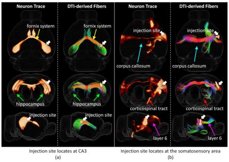
Figure 1.

Two examples of a joint 3D view of neuron tracers and the corresponding DTI derived axonal fibers (with Hausdorff distance smaller than 0.5 mm) from different views. For each sub-figure, 3D rendering of tracer density is shown on the left and the corresponding DTI fiber tracks are shown on the right together with injection sites highlighted by white arrows. A transparent reconstructed cortical surface is also shown in each figure. (a) Injection site locates at CA3. (b) Injection site locates at the somatosensory area.

Relatively small Hausdorff distance between a pair of DTI derived fiber streamline and neuron trace indicates close correlation between them. When the Hausdorff distance of a fiber streamline to a neuron trace is small, it can be concluded that the streamline successfully capture the white matter pathway detected by the neuron tracing experiment. On the other hand, with the large number of neuron tracing experiments in the AMCA covering the whole brain, we premised that the majority of white matter pathways are captured by these experiments. Thus, if a DTI derived fiber streamline is detected to have a relatively large distance to all the neuron tracers, this fiber streamline is possible to be a false tracking. Based on this assumption, the smallest Hausdorff distance (SHD) of each fiber streamline to all the neuron tracing experiments is selected as the best quantifiable value to measure the reliability of DTI tractography. SHDs of all the DTI derived fiber streamlines were computed for quantitative analysis. Notably, as the injection sites only locate on the right hemisphere in the AMCA, the ipsilateral pathways on the left hemisphere were not labeled in these experiments. Thus only those DTI derived axonal fibers that project within/to/from right hemisphere were applied for analysis.

3 Results

3.1 Optimal parcellation scheme and parameters to construct DTI based connectome

ROC curves on different scales with different parameters were shown in Figure 2 and Figure 3 for ipsilateral connection (right hemisphere) and contralateral connection accordingly, and the corresponding AUCs were listed in Table 1. It can be seen that the FA threshold has more impact on reconstructed connectome than the angular threshold. As shown in Table 1, AUCs were relatively higher with small FA threshold (0.1) and large angular threshold (50°–80°). Intuitively, smaller FA threshold and larger angular threshold will result in more fibers and increase the chance to establish connections, as highlighted by green arrows in figures, which results in higher AUCs. However, this may also increase the risk of false positive connections at the same time. On the other hand, an increasing amount of connections were missed by DTI tractography when more restrict tractography thresholds were selected, which results in horizontal lines in Figure 2 and Figure 3. Nevertheless, by looking at the overall trend of ROI curves, a clear tradeoff between sensitivity (true positive rate) and specificity (1 – false positive rate) can be observed when tuning the threshold of fiber numbers and tractography parameters which agrees with the findings in (Thomas et al., 2014). If we only focus locally on ROC curves as highlighted by the red arrows in the figures, we can see that smaller FA threshold (0.1) and angular threshold (40°) gives the best performance – to construct largest number of correct connections with the fewest wrong connections. Thus, we took this parameter as the optimal one. In Figure 4, we compared the obtained brain connectome based on optimal DTI tractography parameters with those none-optimized ones. Specifically, we extracted and highlighted those corrected connections after optimization in Figure 4(d)–(f). It can be seen that a significant amount of connections have been corrected after optimization and suggests that applying optimal DTI tractography parameters is critical in generating accurate result when analyzing brain connectome. The fiber tracts and the corresponding connectome applied for comparison between DTI tractography and neuron tracing in the next sessions were obtained based on this optimal set of parameters.

Figure 2.

ROC curve for DTI derived ipsilateral connectome on the right hemisphere with different parameters using different percolation schemes by taking tracing experiments based connectivity as truth. The fiber tracking termination angle varies from 40 degree to 80 degree. The FA threshold for fiber tracking to start and stop varies from 0.1 to 0.3. For each combination of tractography parameters, a ROC curve is generated with the threshold of fiber number to establish connectivity changes alone the curve. Color legend is shown on the right bottom of each sub-figure. (a),(b),(c): the brain is parcellated into 300, 96, and 69 regions accordingly. (d) When the FA threshold is 0.1, comparisons across different parcellation scales are shown.

Figure 3.

ROC curve for DTI derived contralateral connectome with different parameters using different percolation schemes by taking tracing experiments based connectivity as truth. The fiber tracking termination angle varies from 40 degree to 80 degree. The FA threshold for fiber tracking to start and stop varies from 0.1 to 0.3. For each combination of tractography parameters, a ROC curve is generated with the threshold of fiber number to establish connectivity changes alone the curve. Color legend is shown on right bottom of each sub-figure. (a),(b),(c): the brain is parcellated into 300, 96, and 69 regions accordingly. (d) When the FA threshold is 0.1, comparisons across different parcellation scales are shown.

Table 1.

AUCs of DTI constructed connectome matrix

		Ipsilateral connection					Contralateral connection
Regions	angular	40	50	60	70	80	40	50	60	70	80
	FA
300	0.1	53%	60%	63%	65%	66%	42%	52%	57%	60%	61%
	0.2	41%	45%	48%	50%	52%	26%	32%	36%	39%	42%
	0.3	22%	23%	24%	24%	24%	9%	11%	11%	12%	13%
96	0.1	67%	71%	72%	72%	71%	62%	67%	68%	68%	68%
	0.2	61%	64%	65%	67%	67%	53%	58%	61%	63%	64%
	0.3	46%	47%	48%	48%	49%	30%	32%	33%	35%	36%
69	0.1	68%	70%	69%	70%	69%	64%	65%	66%	65%	64%
	0.2	62%	63%	64%	64%	65%	56%	59%	61%	62%	63%
	0.3	47%	48%	48%	49%	49%	36%	38%	39%	41%	42%

Figure 4.

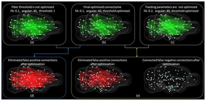
Examples of improvements of DTI derived connectome after parameter optimization. Whole brain is annotated by 96 regions with the center of each one represented by white sphere. (a)–(c): Visualization of ipsilateral connectome derived from DTI tractography when different parameters were selected. Result based on optimal parameters is shown in (b). In (a), threshold of fiber number to establish connection is not optimized and set to 1. In (c), the parameters for fiber tracking are not optimized. (d) Visualization of eliminated false positive connections from the result shown in (a) after optimizing fiber threshold. (e) Visualization of improvements from the result shown in (c) after optimizing tracking parameters.

Meanwhile, it is obvious that DTI performs much better in constructing connectome with coarser anatomical parcellation scheme in comparison with the finest anatomical parcellation scheme. As shown in Table 1 and highlighted by the dark red and pink arrows in Figure 2(d) and Figure 3(d), parceling the mouse brain into 69 regions or 96 regions is more favored over 300 regions to construct brain connectome. Intuitively, for smaller brain region, less DTI-tracked fibers will go through it. With larger brain regions, connections could be more easily captured. However, with more fibers going through a region, the chance to generate wrong connections is also increased at the same time. Thus though DTI performs equally well for 96 regions and 69 regions when larger fiber number threshold was selected as highlighted by the dark/light red arrows in Figure 2(d) and Figure 3(d), the best performance was obtained with 96 regions when smaller fiber number threshold was chosen and denser connections were obtained as highlighted by magenta arrows in both figures. This agrees with the observation based on AUCs in Table 1 that the connectome generated based on middle scale parcellation scheme with 96 regions has the highest AUCs.

In previous analysis, we did not specify the streamline length threshold. To further investigate the impact of streamline lengths on constructing accurate brain connectome, we separated fiber streamlines into 3 groups by their length (0–5mm, 5–10mm, longer than 10mm) and construct whole brain connectome based on different groups using similar approaches as previously. Then by taking tracing data derived connectivity as the truth, their reliability in constructing whole brain connectome were analyzed (Table 2). Interestingly, similar to the findings in (Thomas et al., 2014), different group of fibers has different preference in higher specificity or higher sensitivity. Short streamlines have higher specificity while long streamlines have higher sensitivity (especially for contralateral connections). Another interesting finding is that higher accuracy and precision were obtained with shorter fiber streamlines. Though long distance connection will be missing (false negative) when only considering short fiber streamlines, it will also reduce the number of false positive and increase the number of true negative at the same time. Since in our experiment, long distance connections reconstructed based on neuron tracer are relatively sparse, which means the chance to generate false positive long distance connection is relatively high, high accuracy and precision were obtained when excluding long fiber streamlines in analysis. However, the overall connections identified were reduced by only consider part of the fiber streamlines (reduced AUCs). Thus in successive analysis, the fiber streamlines were not filtered by length.

Table 2.

Analysis of DTI constructed connectome based on different length of streamlines.

Streamline Length		0–5 mm			5–10 mm			> 10 mm			All
Parcellation Scheme		301	96	69	301	96	69	301	96	69	301	96	69
Ipsilateral Connection	Accuracy	81%	72%	70%	74%	62%	57%	71%	56%	49%	72%	73%	72%
	Precision	46%	39%	46%	35%	31%	35%	30%	28%	31%	33%	39%	47%
	Sensitivity	42%	64%	66%	52%	74%	76%	50%	74%	78%	54%	57%	58%
	Specificity	89%	74%	72%	79%	59%	50%	75%	52%	38%	76%	77%	77%
	AUC	40%	59%	61%	48%	64%	65%	45%	61%	62%	53%	67%	68%
Contralateral Connection	Accuracy	85%	83%	80%	81%	72%	69%	72%	57%	49%	72%	67%	64%
	Precision	53%	34%	41%	37%	25%	29%	24%	20%	22%	26%	23%	27%
	Sensitivity	20%	31%	29%	35%	53%	52%	38%	72%	78%	47%	60%	65%
	Specificity	97%	91%	91%	89%	75%	72%	79%	54%	43%	76%	69%	63%
	AUC	19%	30%	29%	34%	49%	48%	34%	59%	61%	42%	62%	64%

3.2 Tract-wise comparison

To evaluate the description power of Hausdorff distance and examine the performance of DTI tractography, we extracted DTI derived fiber streamlines with Hausdorff distances smaller than 0.5 mm to certain neuronal projection tracing for visual analysis (two examples showed in Figure 1 and 10 more examples showed in Figure S4). By visual check, we found that the identified corresponding DTI derived streamlines are close to the neuron tracing result which suggests that Hausdorff distance is powerful in measuring similarity between these two sets of data. On the other side, it can be seen that DTI tractography performs reasonably well in identifying major axonal projection pathways such as the contralateral connections of hippocampus including fornix system (Figure 1(a), the yellow arrows) and the projection pathways from somatosensory area (Figure 1(b)) including corpus callosum (the azure arrows) and corticospinal tract (the red arrows). Intriguingly, in addition to the major white matter pathways, our observation suggested that DTI tractography is also able to infer detailed axonal connections such as the projection from the somatosensory area to the motor area through layer 6 detected by neuron tracer as highlighted by the magenta arrows shown in Figure 1(b).

Our experiments showed that the correspondence can be precisely established between brain pathways identified by neuron tracing experiments and the DTI derived fiber streamlines in the case of small Hausdorff distances (smaller than 0.5mm) and when the Hausdorff distance is larger than 1mm, the correspondence between tracer labeled projections and fiber streamlines is not reliable (Figure 5(e)). By taking SHDs of DTI derived fiber streamlines to tracing experiments as a measurement, the reliability of DTI tractography was examined quantitatively. Our result suggests that most of the DTI derived fibers have relatively small SHDs (Figure 5(a)). 92.9% fibers have SHDs smaller than 0.5 mm and only 0.48% fibers have SHDs larger than 1 mm (Figure 5(d)). This result suggests that DTI is in general reliable (>90% accuracy) in identifying meaningful axonal fibers. It is also worthwhile to examining further the remaining 7.1% of fibers with SHD larger than 1mm as where the causes of false tracking fibers embedded.

Figure 5.

(a) Visualization of fibers projected to/from the right hemisphere. Each fiber is color-coded by its SHD to all the neuron tracer volumes (color bar on the top left). Fibers were set transparent for better visualization. (b) Visualization of all the fibers with SHD larger than 1mm. Fibers are color coded by local orientations. (c) Manually selected fibers that have SHD larger than 1mm from the left main olfactory bulb (MOB) as highlighted by the red circle. (d) Histogram of SHD for all fibers projected to/from the right hemisphere. (e) Visualization of fibers with certain Hausdorff distance to the neuron trace shown on the left.

By our observation, most of these possible false tracking fibers were relatively long and were likely to be caused by the false merging/linking to different pathways (type I error) (Figure 5(b)). To better demonstrate it, we manually extracted those possible false tracking fibers projected from/to the left main olfactory bulb (MOB) and visualized them with white curves in Figure 5(c). It can be seen that most of these fiber streamlines form contralateral projections from/to left MOB. Previous neuron tracing study has pointed that the only efferent projection of MOB to the contralateral half of the brain was to the anterior olfactory nucleus (Shipley and Adamek, 1984), suggesting that those extracted DTI fiber streamlines with large SHDs are likely to be false tracking result – when the projection between MOB and hippocampal formation reconstructed, the algorithm mistakenly linked the streamline to the corpus callosum tracts and fornix system tracts, as highlighted by the dashed curves and red crosses in Figure 5(c).

In addition to the above mentioned false connections (type I error), we also noticed false breaks (type II error) that cannot be detected by SHD in our analysis. For instance, in Figure 1(b), though the corticalspinal tract has been successfully reconstructed by DTI tractography, if we manually highlight those corticalspinal tracts (Figure 6(a)), a clear gap was observed between the tract and the isocortex. As a result, the connection between somatosensory area and the spinal regions identified by neuron tracers were not identified by DTI tractography. Another example is the efferent projection from nucleus of reunions (RE) to hippocampal formations such as the entorhinal area (ENT) or CA1 (Herkenham, 1978) identified by neuron tracers (highlighted by magenta curves in Figure 6(c)). Even though, the pathway has been partially identified by DTI derived axonal fibers, as highlighted by different colors in Figure 6(b), the pathway is composed by disjoint segments of DTI derived fibers. Thus no direct connection between RE and hippocampal formations can be identified by DTI tractography. Nevertheless, such type II error will be ignored by morphology descriptor such as SHDs proposed and can only be detected by analyzing regional connections. Facing such problem, in the next session, whole brain connectome in large scale will be compared between two sets of data to count both types of error globally and guide the selection of optimal parameters.

Figure 6.

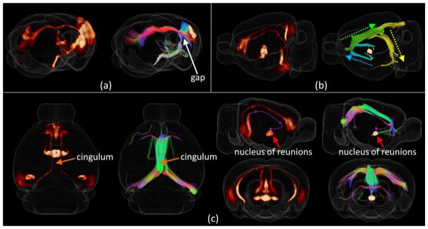
3D visualizations of the neuron tracing volume (left) and the corresponding fiber tracks (right) with type II error. (a) For the study shown in Figure 1(b), cortical-spinal projections were manually selected and highlighted by the white curves. A gap can be clearly observed between fiber streamlines and the cortex as highlighted by the white arrow. (b)–(c) A neuron tracing study with injection site locates in the nucleus of reunions (RE). As highlighted by the magenta dash curve, the connection follows the cingulum and is projected to the entorhinal area and CA1. Though the corresponding DTI streamlines were identified successfully, it is broken down into 3 segments as represented by the azure, green, and yellow curves shown in (b).

3.3 Connectome-wise comparison

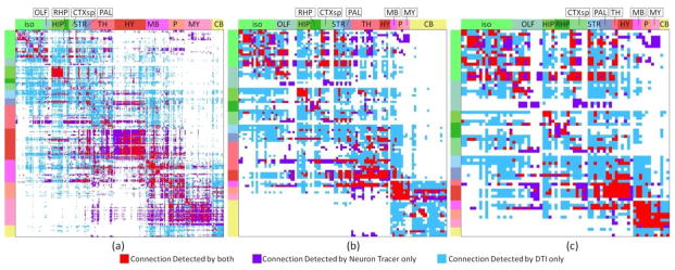
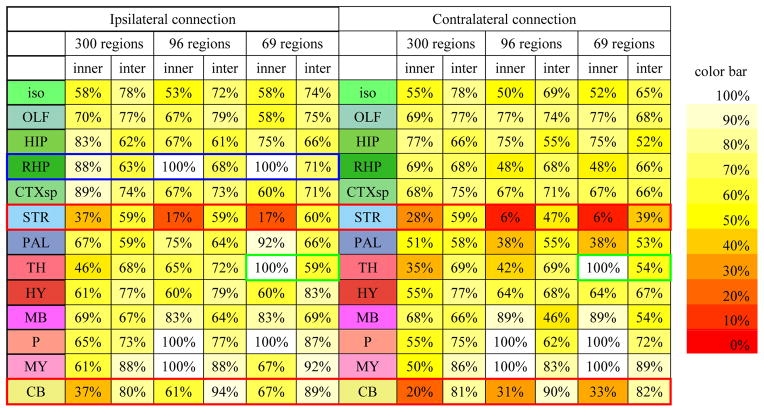
We then compared the obtained connectomes on different scales based on neuron tracing and DTI data. We jointly visualized the binarized connectome matrices obtained based on DTI and neuron tracing in different annotation scales for ipsilateral connection (Figure 7) and contralateral connection (Figure 8). Intriguing, by visual check, we can see that DTI performs better in constructing ipsilateral connection than contralateral connection. Similar observation can also be obtained by comparing ROC curves in Figure 2 and Figure 3 and the AUCs in Table 1. It is also evident that a considerable amount of errors have been generated by DTI. Though DTI performs reasonably well when constructing connectome based on optimal parameters, we could still see a considerable amount of disagreement between DTI derived connectome and neuron tracing derived connectome. For further analysis, we then clustered regions by their anatomical locations and computed the accuracy of DTI in constructing inner cluster connections and intra cluster connections. The result is shown in Table 3. The overall performance of DTI is relatively good across the whole brain. However, as highlighted by the red boxes, DTI displayed poor performance in constructing connections for stratium (STR) and cerebellum (CB). For STR, this is partially because it is surrounded by white matter fiber pathways and penetrated by axonal fiber bundles which are more easily identified by DTI as connected via axonal fibers. Thus more connections than expected were identified in this region that resulted in overwhelmed false positive connections. However, as for cerebellum, it is partially because only a few neuron tracing experiments (40) has been taken in current released of AMCA and relatively small dose neuron tracer was injected for some of them. As a result, fewer connections than reality were identified for brain regions in the cerebellum and current incomplete data cannot tell us much on DTI’s performance in the cerebellum. On the other side, as highlighted by the green box, DTI performed relatively well in identifying ipsilateral connections for retrohippocampal region (RHP), while performed relatively poor for contralateral connections. This is partially because RHP locates at the lateral part of the brain and long distance connections are required to form contralateral connections which DTI tractography failed to construct. On the contrary, for regions locate at the hindbrain that is close to brain midline (e.g. pons (P), medulla (MY)), DTI performs equally well to construct both ipsilateral and contralateral connections in coarser scale.

Figure 7.

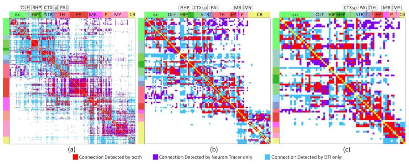
Comparison of mouse brain ipsilateral connectome derived from neuron tracer or DTI using different percolation schemes. For neuron tracer, when the p-value of correlation coefficient between an injection site and a projection site is larger than 0.05, the projection will be identified as from the injection site to the projection site. For DTI, when number of fibers connected between two regions is larger than the threshold, these two regions were identified as being connected. The optimal threshold is selected based on the ROC curve accordingly. DTI tractography was performed based on the following parameters: FA threshold: 0.1, angular threshold 40. (a) 300 regions. (b) 96 regions. (c) 69 regions. The red color represents common connections detected by both approaches. The violet color represents connections detected by neuron tracer only. The azure color represents connections detected by DTI only.

Figure 8.

Comparison of mouse brain contralateral connectome derived from neuron tracer or DTI using different percolation schemes. For neuron tracer, when the p-value of correlation coefficient between an injection site and a projection site is larger than 0.05, the projection will be identified as from the injection site to the projection site. For DTI, when the number of fibers connected between two regions is larger than the threshold, these two regions were identified as connected. The optimal threshold is selected based on the ROC curve accordingly. DTI tractography was performed based on the following parameters: FA threshold: 0.1, angular threshold 40. (a) 300 regions. (b) 96 regions. (c) 69 regions. The red color represents common connections detected by both approaches. The violet color represents connections detected by neuron tracer only. The azure color represents connections detected by DTI only.

Table 3.

Accuracy of DTI constructed connectome for inner and inter regional connections.

4 Discussion

By taking neuron tracing data in mouse brain in the AMCA as a validation tool, we have investigated the performance of whole brain DTI tractography and the corresponding large-scale connectome. A novel framework was presented for quantitative comparison between DTI data and tracing data. With quantitative measurement, we showed that over ninety percent DTI derived axonal fibers could identify corresponding fiber pathways, which suggested that DTI is a reliable tool in studying major brain pathways. Yet we have revealed that the optimal parameters and the right scale of parcellation scheme are critical in constructing a reliable large-scale brain connectome. In comparison with angular threshold, FA threshold was shown having more impact on DTI tractography result. In our case, small FA threshold (0.1) generated the best result which agrees with the other’s work (Dauguet et al., 2007). Our results also suggested that to construct large-scale connectome, right parcellation scheme is very important and the size of analyzed brain regions should neither be too small nor too big. For our data, annotating mouse brain with 96 regions is the best in comparison with finer and coarser parcellation schemes. With the optimal parameters, the overall performance of DTI tractography is reasonably good in constructing large-scale connectome.

Overall, DTI can be a substantially more reliable tool to investigate brain connectome on the conditions that optimal parameters and the appropriate parcellation scheme were carefully selected. Nevertheless, our framework still detected type I and type II errors with DTI tractography. This agrees with the findings in macaque brain in (Thomas et al., 2014). Not surprisingly, a considerable amount of disagreement between DTI constructed connectome and neuron tracing constructed connectome – especially in the contralateral connections and the connections of striatum and cerebellum – were noted. Though some type I errors can be accounted by the incompleteness of the neuron tracing data set such as those in the cerebellum, most of them might result from the inaccuracy of DTI tractography. These errors could be potentially caused by the complex wiring pattern in the brain (Jbabdi and Johansen-Berg, 2011) that cannot be modeled by the classic diffusion tensor model applied in this work. Notably, more comprehensive multi-orientation models such as Q-ball (Hess et al., 2006; Tuch, 2004), DSI tractography (Wedeen et al., 2008, 2005), or susceptibility tensor imaging (STI) (Liu et al., 2012) could be used to reduce the possibility of such breaking or missing fibers by considering fiber bundle cross in the model. On the other hand, instead of the limited accuracy of DTI tractography, some errors could also be caused by the registration error. Since it is quite challenging to register images from different modalities and there is zig-zag effect in stitched sections of AMRA, current study applied linear registration and images were not perfectly aligned before analysis. Thus, with specially designed registration algorithm dedicated to this problem and the better quality data, it would be interesting to benchmark and compare the advanced tracing models on their performance in constructing fiber pathways (Fillard et al., 2011) and whole brain connectome and to investigate the effect of individual variability and acquisition variability on tractography results.

Notably, the evaluation of DTI tractography obtained based on the proposed framework may not be readily applicable to human brains at the current stage. Given the significant differences between the nature of human brain and mouse brain such as size and anatomical structures, it is still an open question on how to link the findings in the brain of these two species. From DTI data acquisition perspective, the image resolution is also very different (e.g. mouse: 50–100 micron resolution (Calamante et al., 2012; Zhang et al., 2002), human: 1–3 mm resolution (Hansen et al., 2011; Sotiropoulos et al., 2013)), thus the microstructures inferred by tractography in mouse and human brains have a magnitude difference (Mori and Zhang, 2006; Xu et al., 2008). Also, the DTI data in mouse brains is post-mortem which allows long scanning time for more details and low SNR, but it will influence water molecule diffusion properties in comparison with live brain applied in human study at the same time. However, the principles and methods of dMRI and the tractography approaches are virtually the same in all animal models. The findings in this paper largely agree with the recent findings in macaque brain which is more comparable to human brain that dMRI tractography has limited accuracy in inferring brain structural connections and there is tradeoff between sensitivity and specificity (Thomas et al., 2014). It is noteworthy to mention that the study in macaque brain was limited to only two tracer injections. By comparison, our proposed framework and the corresponding findings are based on the AMCA dataset which includes 1772 tracer injections that covers the whole brain. Our proposed framework can be applied as a reliable test bed for dMRI tractography, and should be generally applicable to the assessments of the performance of advanced dMRI approaches, guiding a better design of tractography algorithms, and the optimization of parameters and parcellation schemes. On a higher level, as mammal animals, the mouse brain still shares certain level of common anatomy and function mechanisms as the human brain (Song et al., 2014) which is an importance source of knowledge in understanding brain mechanisms. And to fully understand brain mechanisms, it is more desired to validate findings in different scales, different modalities, and different animal models including mouse (e.g. Jbabdi et al., 2013; Jiang, 2013; Rilling et al., 2008; Zhang et al., 2013).

Most importantly, based on our findings, we would like to draw attention to those studies that rely solely on DTI tractography to study brain connections: DTI can be a substantially more reliable and useful tool with optimized tractography parameters and brain parcellation schemes. If these conditions are not met and the performance is not tested, DTI-generated connection maps may contain numbers of the potential errors which can lead to erroneous conclusions.

Highlights.

1. Joint evaluation of DTI and neuron tracing data.

2. Performance of whole brain DTI tractography has been evaluated by ground truth.

3. With optimized parameters and scales, we can substantially more confidently trust DTI.

4. Serving as a ground truth method to facilitate the development of novel fiber tracking algorithms.

References

- Assaf Y, Alexander DC, Jones DK, Bizzi A, Behrens TEJ, Clark CA, Cohen Y, Dyrby TB, Huppi PS, Knoesche TR, Lebihan D, Parker GJM, Poupon C, Anaby D, Anwander A, Bar L, Barazany D, Blumenfeld-Katzir T, De-Santis S, Duclap D, Figini M, Fischi E, Guevara P, Hubbard P, Hofstetter S, Jbabdi S, Kunz N, Lazeyras F, Lebois A, Liptrot MG, Lundell H, Mangin JF, Dominguez DM, Morozov D, Schreiber J, Seunarine K, Nava S, Riffert T, Sasson E, Schmitt B, Shemesh N, Sotiropoulos SN, Tavor I, Zhang HG, Zhou FL. The CONNECT project: Combining macro- and micro-structure. Neuroimage. 2013;80:273–82. doi: 10.1016/j.neuroimage.2013.05.055. [DOI] [PubMed] [Google Scholar]
- Assaf Y, Pasternak O. Diffusion tensor imaging (DTI)-based white matter mapping in brain research: a review. J Mol Neurosci. 2008;34:51–61. doi: 10.1007/s12031-007-0029-0. [DOI] [PubMed] [Google Scholar]
- Basser PJ, Mattiello J, LeBihan D. MR diffusion tensor spectroscopy and imaging. Biophys J. 1994;66:259–67. doi: 10.1016/S0006-3495(94)80775-1. [DOI] [PMC free article] [PubMed] [Google Scholar]
- Bassett DS, Bullmore ET. Human brain networks in health and disease. Curr Opin Neurol. 2009;22:340–7. doi: 10.1097/WCO.0b013e32832d93dd. [DOI] [PMC free article] [PubMed] [Google Scholar]
- Bullmore E, Sporns O. Complex brain networks: graph theoretical analysis of structural and functional systems. Nat Rev Neurosci. 2009;10:186–98. doi: 10.1038/nrn2575. [DOI] [PubMed] [Google Scholar]
- Calamante F, Tournier JD, Kurniawan ND, Yang Z, Gyengesi E, Galloway GJ, Reutens DC, Connelly A. Super-resolution track-density imaging studies of mouse brain: comparison to histology. Neuroimage. 2012;59:286–96. doi: 10.1016/j.neuroimage.2011.07.014. [DOI] [PubMed] [Google Scholar]
- Chen H, Zhang T, Guo L, Li K, Yu X, Li L, Hu XX, Han J, Liu T. Coevolution of gyral folding and structural connection patterns in primate brains. Cereb Cortex. 2013;23:1208–17. doi: 10.1093/cercor/bhs113. [DOI] [PMC free article] [PubMed] [Google Scholar]
- Choe AS, Stepniewska I, Colvin DC, Ding Z, Anderson AW. Validation of diffusion tensor MRI in the central nervous system using light microscopy: quantitative comparison of fiber properties. NMR Biomed. 2012;25:900–8. doi: 10.1002/nbm.1810. [DOI] [PMC free article] [PubMed] [Google Scholar]
- Côté MA, Girard G, Boré A, Garyfallidis E, Houde JC, Descoteaux M. Tractometer: towards validation of tractography pipelines. Med Image Anal. 2013;17:844–57. doi: 10.1016/j.media.2013.03.009. [DOI] [PubMed] [Google Scholar]
- Dauguet J, Peled S, Berezovskii V, Delzescaux T, Warfield SK, Born R, Westin CF. Comparison of fiber tracts derived from in-vivo DTI tractography with 3D histological neural tract tracer reconstruction on a macaque brain. Neuroimage. 2007;37:530–8. doi: 10.1016/j.neuroimage.2007.04.067. [DOI] [PubMed] [Google Scholar]
- Dyrby TB, Søgaard LV, Parker GJ, Alexander DC, Lind NM, Baaré WFC, Hay-Schmidt A, Eriksen N, Pakkenberg B, Paulson OB, Jelsing J. Validation of in vitro probabilistic tractography. Neuroimage. 2007;37:1267–77. doi: 10.1016/j.neuroimage.2007.06.022. [DOI] [PubMed] [Google Scholar]
- Fillard P, Descoteaux M, Goh A, Gouttard S, Jeurissen B, Malcolm J, Ramirez-Manzanares A, Reisert M, Sakaie K, Tensaouti F, Yo T, Mangin JF, Poupon C. Quantitative evaluation of 10 tractography algorithms on a realistic diffusion MR phantom. Neuroimage. 2011;56:220–34. doi: 10.1016/j.neuroimage.2011.01.032. [DOI] [PubMed] [Google Scholar]
- Gao Y, Choe AS, Stepniewska I, Li X, Avison MJ, Anderson AW. Validation of DTI tractography-based measures of primary motor area connectivity in the squirrel monkey brain. PLoS One. 2013;8:e75065. doi: 10.1371/journal.pone.0075065. [DOI] [PMC free article] [PubMed] [Google Scholar]
- Hansen B, Flint JJ, Heon-Lee C, Fey M, Vincent F, King MA, Vestergaard-Poulsen P, Blackband SJ. Diffusion tensor microscopy in human nervous tissue with quantitative correlation based on direct histological comparison. Neuroimage. 2011;57:1458–65. doi: 10.1016/j.neuroimage.2011.04.052. [DOI] [PMC free article] [PubMed] [Google Scholar]
- Herkenham M. The connections of the nucleus reuniens thalami: evidence for a direct thalamo-hippocampal pathway in the rat. J Comp Neurol. 1978;177:589–610. doi: 10.1002/cne.901770405. [DOI] [PubMed] [Google Scholar]
- Hess CP, Mukherjee P, Han ET, Xu D, Vigneron DB. Q-ball reconstruction of multimodal fiber orientations using the spherical harmonic basis. Magn Reson Med. 2006;56:104–17. doi: 10.1002/mrm.20931. [DOI] [PubMed] [Google Scholar]
- Huttenlocher DP, Klanderman GA, Rucklidge WJ. Comparing images using the Hausdorff distance. IEEE Trans Pattern Anal Mach Intell. 1993;15:850–863. doi: 10.1109/34.232073. [DOI] [Google Scholar]
- Jbabdi S, Johansen-Berg H. Tractography: where do we go from here? Brain Connect. 2011;1:169–83. doi: 10.1089/brain.2011.0033. [DOI] [PMC free article] [PubMed] [Google Scholar]
- Jbabdi S, Lehman JF, Haber SN, Behrens TE. Human and monkey ventral prefrontal fibers use the same organizational principles to reach their targets: tracing versus tractography. J Neurosci. 2013;33:3190–201. doi: 10.1523/JNEUROSCI.2457-12.2013. [DOI] [PMC free article] [PubMed] [Google Scholar]
- Jenkinson M, Smith S. A global optimisation method for robust affine registration of brain images. Med Image Anal. 2001;5:143–156. doi: 10.1016/s1361-8415(01)00036-6. [DOI] [PubMed] [Google Scholar]
- Jiang H, van Zijl PCM, Kim J, Pearlson GD, Mori S. DtiStudio: resource program for diffusion tensor computation and fiber bundle tracking. Comput Methods Programs Biomed. 2006;81:106–16. doi: 10.1016/j.cmpb.2005.08.004. [DOI] [PubMed] [Google Scholar]
- Jiang T. Brainnetome: a new -ome to understand the brain and its disorders. Neuroimage. 2013;80:263–72. doi: 10.1016/j.neuroimage.2013.04.002. [DOI] [PubMed] [Google Scholar]
- Jiang T. Brainnetome and related projects. Sci China Life Sci. 2014;57:462–6. doi: 10.1007/s11427-014-4642-1. [DOI] [PubMed] [Google Scholar]
- Leergaard TB, White NS, de Crespigny A, Bolstad I, D’Arceuil H, Bjaalie JG, Dale AM. Quantitative histological validation of diffusion MRI fiber orientation distributions in the rat brain. PLoS One. 2010;5:e8595. doi: 10.1371/journal.pone.0008595. [DOI] [PMC free article] [PubMed] [Google Scholar]
- Li L, Hu X, Preuss TM, Glasser MF, Damen FW, Qiu Y, Rilling J. Mapping putative hubs in human, chimpanzee and rhesus macaque connectomes via diffusion tractography. Neuroimage. 2013;80:462–474. doi: 10.1016/j.neuroimage.2013.04.024. [DOI] [PMC free article] [PubMed] [Google Scholar]
- Liu C, Li W, Wu B, Jiang Y, Johnson GA. 3D fiber tractography with susceptibility tensor imaging. Neuroimage. 2012;59:1290–8. doi: 10.1016/j.neuroimage.2011.07.096. [DOI] [PMC free article] [PubMed] [Google Scholar]
- Logothetis NK. What we can do and what we cannot do with fMRI. Nature. 2008;453:869–78. doi: 10.1038/nature06976. [DOI] [PubMed] [Google Scholar]
- Meskaldji DE, Fischi-Gomez E, Griffa A, Hagmann P, Morgenthaler S, Thiran JP. Comparing connectomes across subjects and populations at different scales. Neuroimage. 2013;80:416–25. doi: 10.1016/j.neuroimage.2013.04.084. [DOI] [PubMed] [Google Scholar]
- Moldrich RX, Pannek K, Hoch R, Rubenstein JL, Kurniawan ND, Richards LJ. Comparative mouse brain tractography of diffusion magnetic resonance imaging. Neuroimage. 2010;51:1027–36. doi: 10.1016/j.neuroimage.2010.03.035. [DOI] [PMC free article] [PubMed] [Google Scholar]
- Mori S, Crain BJ, Chacko VP, Van Zijl PCM. Three-dimensional tracking of axonal projections in the brain by magnetic resonance imaging. Ann Neurol. 1999;45:265–269. doi: 10.1002/1531-8249(199902)45:2<265::AID-ANA21>3.0.CO;2-3. [DOI] [PubMed] [Google Scholar]
- Mori S, Oishi K, Jiang H, Jiang L, Li X, Akhter K, Hua K, Faria AV, Mahmood A, Woods R, Toga AW, Pike GB, Neto PR, Evans A, Zhang J, Huang H, Miller MI, van Zijl P, Mazziotta J. Stereotaxic white matter atlas based on diffusion tensor imaging in an ICBM template. Neuroimage. 2008;40:570–82. doi: 10.1016/j.neuroimage.2007.12.035. [DOI] [PMC free article] [PubMed] [Google Scholar]
- Mori S, Zhang J. Principles of Diffusion Tensor Imaging and Its Applications to Basic Neuroscience Research. Neuron. 2006;51:527–39. doi: 10.1016/j.neuron.2006.08.012. [DOI] [PubMed] [Google Scholar]
- NIH. Working Group Report to the Advisory Committee to the Director. NIH; 2014. BRAIN 2025: A Scientific Vision - Brain Research through Advancing Innovative Neurotechnologies (BRAIN) [Google Scholar]
- Oh SW, Harris JA, Ng L, Winslow B, Cain N, Mihalas S, Wang Q, Lau C, Kuan L, Henry AM, Mortrud MT, Ouellette B, Nguyen TN, Sorensen SA, Slaughterbeck CR, Wakeman W, Li Y, Feng D, Ho A, Nicholas E, Hirokawa KE, Bohn P, Joines KM, Peng H, Hawrylycz MJ, Phillips JW, Hohmann JG, Wohnoutka P, Gerfen CR, Koch C, Bernard A, Dang C, Jones AR, Zeng H. A mesoscale connectome of the mouse brain. Nature. 2014;508:207–14. doi: 10.1038/nature13186. [DOI] [PMC free article] [PubMed] [Google Scholar]
- Ragan T, Kadiri LR, Venkataraju KU, Bahlmann K, Sutin J, Taranda J, Arganda-Carreras I, Kim Y, Seung HS, Osten P. Serial two-photon tomography for automated ex vivo mouse brain imaging. Nat Methods. 2012;9:255–8. doi: 10.1038/nmeth.1854. [DOI] [PMC free article] [PubMed] [Google Scholar]
- Rilling JK, Glasser MF, Preuss TM, Ma X, Zhao T, Hu X, Behrens TEJ. The evolution of the arcuate fasciculus revealed with comparative DTI. Nat Neurosci. 2008;11:426–8. doi: 10.1038/nn2072. [DOI] [PubMed] [Google Scholar]
- Seehaus AK, Roebroeck A, Chiry O, Kim DS, Ronen I, Bratzke H, Goebel R, Galuske RAW. Histological validation of DW-MRI tractography in human postmortem tissue. Cereb Cortex. 2013;23:442–50. doi: 10.1093/cercor/bhs036. [DOI] [PMC free article] [PubMed] [Google Scholar]
- Shipley MT, Adamek GD. the connections of the mouse olfactory bulb: A study using orthograde and retrograde transport of wheat germ agglutinin conjugated to horseradish peroxidase. Brain Res Bull. 1984;12:669–688. doi: 10.1016/0361-9230(84)90148-5. [DOI] [PubMed] [Google Scholar]
- Song HF, Kennedy H, Wang XJ. Spatial embedding of structural similarity in the cerebral cortex. Proc Natl Acad Sci. 2014;111:16580–16585. doi: 10.1073/pnas.1414153111. [DOI] [PMC free article] [PubMed] [Google Scholar]
- Sotiropoulos SN, Jbabdi S, Xu J, Andersson JL, Moeller S, Auerbach EJ, Glasser MF, Hernandez M, Sapiro G, Jenkinson M, Feinberg DA, Yacoub E, Lenglet C, Van Essen DC, Ugurbil K, Behrens TEJ. Advances in diffusion MRI acquisition and processing in the Human Connectome Project. Neuroimage. 2013;80:125–43. doi: 10.1016/j.neuroimage.2013.05.057. [DOI] [PMC free article] [PubMed] [Google Scholar]
- Sporns O, Tononi G, Kötter R. The human connectome: A structural description of the human brain. PLoS Comput Biol. 2005;1:e42. doi: 10.1371/journal.pcbi.0010042. [DOI] [PMC free article] [PubMed] [Google Scholar]
- Thomas C, Frank Q. Anatomical accuracy of brain connections derived from diffusion MRI tractography is inherently limited. Proc. …. 2014 doi: 10.1073/pnas.1405672111. [DOI] [PMC free article] [PubMed] [Google Scholar]
- Thomas C, Ye FQ, Irfanoglu MO, Modi P, Saleem KS, Leopold DA, Pierpaoli C. Anatomical accuracy of brain connections derived from diffusion MRI tractography is inherently limited. Proc Natl Acad Sci. 2014;111:16574–16579. doi: 10.1073/pnas.1405672111. [DOI] [PMC free article] [PubMed] [Google Scholar]
- Tsien JZ, Li M, Osan R, Chen G, Lin L, Wang PL, Frey S, Frey J, Zhu D, Liu T, Zhao F, Kuang H. On initial Brain Activity Mapping of episodic and semantic memory code in the hippocampus. Neurobiol Learn Mem. 2013;105:200–10. doi: 10.1016/j.nlm.2013.06.019. [DOI] [PMC free article] [PubMed] [Google Scholar]
- Tuch DS. Q-ball imaging. Magn Reson Med. 2004;52:1358–72. doi: 10.1002/mrm.20279. [DOI] [PubMed] [Google Scholar]
- Tuch DS, Reese TG, Wiegell MR, Makris N, Belliveau JW, Wedeen VJ. High angular resolution diffusion imaging reveals intravoxel white matter fiber heterogeneity. Magn Reson Med. 2002;48:577–82. doi: 10.1002/mrm.10268. [DOI] [PubMed] [Google Scholar]
- Van Essen DC. Cartography and connectomes. Neuron. 2013;80:775–90. doi: 10.1016/j.neuron.2013.10.027. [DOI] [PMC free article] [PubMed] [Google Scholar]
- Van Essen DC, Ugurbil K, Auerbach E, Barch D, Behrens TEJ, Bucholz R, Chang A, Chen L, Corbetta M, Curtiss SW, Della Penna S, Feinberg D, Glasser MF, Harel N, Heath AC, Larson-Prior L, Marcus D, Michalareas G, Moeller S, Oostenveld R, Petersen SE, Prior F, Schlaggar BL, Smith SM, Snyder AZ, Xu J, Yacoub E. The Human Connectome Project: a data acquisition perspective. Neuroimage. 2012;62:2222–31. doi: 10.1016/j.neuroimage.2012.02.018. [DOI] [PMC free article] [PubMed] [Google Scholar]
- Wedeen VJ, Hagmann P, Tseng WYI, Reese TG, Weisskoff RM. Mapping complex tissue architecture with diffusion spectrum magnetic resonance imaging. Magn Reson Med. 2005;54:1377–86. doi: 10.1002/mrm.20642. [DOI] [PubMed] [Google Scholar]
- Wedeen VJ, Wang RP, Schmahmann JD, Benner T, Tseng WYI, Dai G, Pandya DN, Hagmann P, D’Arceuil H, de Crespigny AJ. Diffusion spectrum magnetic resonance imaging (DSI) tractography of crossing fibers. Neuroimage. 2008;41:1267–77. doi: 10.1016/j.neuroimage.2008.03.036. [DOI] [PubMed] [Google Scholar]
- Xu J, Sun SW, Naismith RT, Snyder AZ, Cross AH, Song SK. Assessing optic nerve pathology with diffusion MRI: from mouse to human. NMR Biomed. 2008;21:928–40. doi: 10.1002/nbm.1307. [DOI] [PMC free article] [PubMed] [Google Scholar]
- Zalesky A, Fornito A, Harding IH, Cocchi L, Yücel M, Pantelis C, Bullmore ET. Whole-brain anatomical networks: does the choice of nodes matter? Neuroimage. 2010;50:970–83. doi: 10.1016/j.neuroimage.2009.12.027. [DOI] [PubMed] [Google Scholar]
- Zhang D, Guo L, Zhu D, Li K, Li L, Chen H, Zhao Q, Hu X, Liu T. Diffusion tensor imaging reveals evolution of primate brain architectures. Brain Struct Funct. 2013;218:1429–1450. doi: 10.1007/s00429-012-0468-4. [DOI] [PMC free article] [PubMed] [Google Scholar]
- Zhang H, Schneider T, Wheeler-Kingshott CA, Alexander DC. NODDI: practical in vivo neurite orientation dispersion and density imaging of the human brain. Neuroimage. 2012;61:1000–16. doi: 10.1016/j.neuroimage.2012.03.072. [DOI] [PubMed] [Google Scholar]
- Zhang J, van Zijl PCM, Mori S. Three-dimensional diffusion tensor magnetic resonance microimaging of adult mouse brain and hippocampus. Neuroimage. 2002;15:892–901. doi: 10.1006/nimg.2001.1012. [DOI] [PubMed] [Google Scholar]
Associated Data
This section collects any data citations, data availability statements, or supplementary materials included in this article.