Co-registration and distortion correction of diffusion and anatomical images based on inverse contrast normalization

Abstract

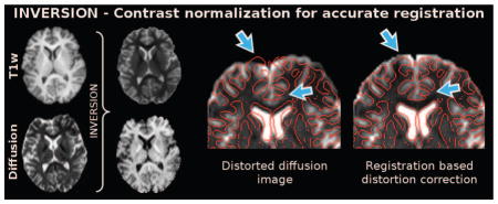
Diffusion MRI provides quantitative information about microstructural properties which can be useful in neuroimaging studies of the human brain. Echo planar imaging (EPI) sequences, which are frequently used for acquisition of diffusion images, are sensitive to inhomogeneities in the primary magnetic (B₀) field that cause localized distortions in the reconstructed images. We describe and evaluate a new method for correction of susceptibility-induced distortion in diffusion images in the absence of an accurate B₀ fieldmap. In our method, the distortion field is estimated using a constrained non-rigid registration between an undistorted T1-weighted anatomical image and one of the distorted EPI images from diffusion acquisition. Our registration framework is based on a new approach, INVERSION (Inverse contrast Normalization for VERy Simple registratION), which exploits the inverted contrast relationship between T1-and T2-weighted brain images to define a simple and robust similarity measure. We also describe how INVERSION can be used for rigid alignment of diffusion images and T1-weighted anatomical images. Our approach is evaluated with multiple in vivo datasets acquired with a different acquisition parameters. Compared to other methods, INVERSION shows robust and consistent performance in rigid registration and shows improved alignment of diffusion and anatomical images relative to normalized mutual information for non-rigid distortion correction.

Graphical abstract

1. Introduction

Diffusion MRI is a non-invasive imaging technique that can provide quantitative and qualitative information about microstructural tissue properties in vivo [1–3]. Quantitative information about diffusion processes can be combined with T1-weighted anatomical images in order to identify, delineate, and quantify the microstructural characteristics of neuro-anatomical structures and the white matter connections between them. In order to jointly analyze these images, they must first be co-registered [4, 5].

There are two primary challenges in accurate co-registration of T1-weighted and diffusion images. First, diffusion MRI frequently uses Echo Planar Imaging (EPI) for data acquisition, which results in localized susceptibility-induced distortions in the reconstructed diffusion weighted images (DWIs) as a result of inhomogeneities in the primary magnetic (B₀) field. These distortions can be particularly pronounced in regions where susceptibility is rapidly changing, such as at the interfaces of soft tissue, air and bone [4, 6, 7]. Second, co-registration of T1-weighted and diffusion images (distorted or undistorted) is difficult because the images are sensitive to different physical properties of the underlying tissue and exhibit very different image contrast. This makes it an inter-modal registration problem [8–10]. When an accurate estimate of the B₀ fieldmap is available, several methods can be employed for accurate correction of the localized susceptibility-induced EPI distortion [6, 11–19]. However, accurate B₀ fieldmap information is not available in many neuroimaging studies and in this paper we present a registration-based method for EPI distortion correction in absence of a fieldmap.

In registration-based methods the distortion field is generally estimated by a non-rigid alignment of the distorted EPI image with no diffusion weighting (i.e. a T2-weighted (T2W) EPI image with a diffusion b-value of 0 s/mm²) to an anatomical image with negligible geometric distortion [20–28]. A T2W-EPI image is commonly used for this purpose because it shows similar image structure to an anatomical image, is almost always acquired in quantitative diffusion studies and manifests very similar distortion as different DWIs [23–28]. Most methods use a T2-weighted anatomical image since these have similar contrast to the T2W-EPI image [20–22, 24–26]. In our approach we use T1-weighted anatomical images as they are frequently acquired in brain-mapping studies to delineate cortex and sub-cortical anatomical structures. Since the contrast of a T1-weighted anatomical image is different from that of the T2W-EPI image, previous approaches [23, 27, 28] use standard inter-modality cost functions that are insensitive to contrast differences (e.g., mutual information (MI) [29–31] or correlation ratio (CR) [32]). Both MI and CR lead to non-convex and non-smooth optimization problems that can be challenging to solve [8–10, 33–36]. In this paper we propose a new approach, INVERSION (Inverse contrast Normalization for VERy Simple registratION), that exploits the approximately inverted contrast relationship between T1- and T2-weighted brain images to transform the contrast of one image into the contrast of the other. This means that the complicated inter-modal registration problem can be simplified to an intra-modal registration problem, which is easier to solve and is less sensitive to highly-misaligned images. We use INVERSION both for co-registration of T1-weighted anatomical and diffusion images and for fieldmap-free susceptibility-induced distortion correction¹.

INVERSION is similar in concept to previous methods that estimate synthetic image contrast [38–45]. Specifically, some MRI-PET [38] and MRI-ultrasound [39] co-registration methods also use image contrast transformations, though these transformations are generally quite complicated and depend on an initial tissue segmentation. Choi et al. [40] use a similar contrast transformation to enhance registration-based distortion correction, but do not use physics-based constraints on the non-rigid deformation field [6, 20]. Other approaches use a multiple-contrast atlas to estimate image intensities for different modalities, either using a non-rigid registration framework [41] or using a patch-based sparse intensity prediction approach [42]. These approaches require solving large optimization problems, whereas INVERSION is computationally cheaper and does not require the construction of an atlas. INVERSION also has similarities to a histogram bin transformation approach [43] for registration of MRI and CT images, although that approach requires user interaction to setup the intensity bin mapping between the histograms of the images while INVERSION is completely automated. In other similar registration methods, a contrast relationship is estimated by using the joint histogram [44] or by assuming a polynomial relationship between the intensities of different images [45]. Both these approaches perform nicely when the registration parameters are initialized well, but poorly otherwise. INVERSION uses an intensity mapping that matches the histograms of the two images so that registration works well even for large displacements between the two images.

The methods described in this paper are implemented in the BrainSuite Diffusion Pipeline (BDP) software, freely available from http://brainsuite.org/. Since conventional inter-modality registration approaches perform well when they have good initializations [33, 35], also seen in our evaluations (section 3), we use Normalized Mutual Information (NMI) [31] based registration to further refine the deformation field estimated by INVERSION approach in our software implementation. This makes the whole registration framework in BDP robust to large misalignment and aligns the images accurately. Note that in this paper we are only interested in evaluating the performance of INVERSION alone and we do not use NMI based registration after INVERSION in any of the results except Fig. 5. BDP also includes multiple methods for modeling diffusion processes such as diffusion tensor and orientation distribution functions.

Figure 5.

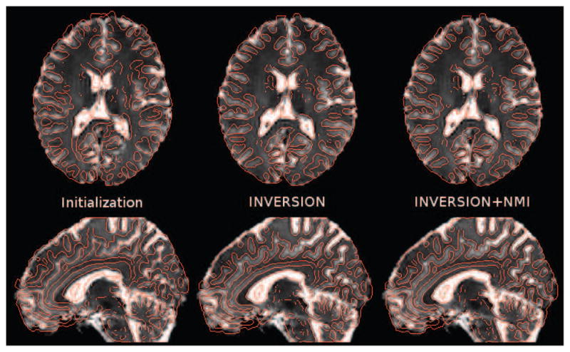
Result of the rigid registration procedure an in vivo image from Dataset-2 dataset (after distortion correction using fieldmap). The T2W-EPI image is overlaid by edge maps from the MPRAGE image in red (left) after initialization, (center) after INVERSION, and (right) after NMI-based refinement. NMI-based refinement adds a very subtle improvement which can be best noticed around edges of ventricles. Note that all other results presented in this paper do not use any NMI-based refinement.

2. Material and methods

EPI images can contain geometric distortions in the presence of B₀ inhomogeneity. Fig. 1 shows an in vivo example: while the T1-weighted image has negligible geometric distortion, the T2W-EPI image is substantially distorted. This leads to discrepancies between the two images when they are rigidly aligned to each other without distortion correction. Specifically, it can be noticed that image edges do not align correctly in distorted regions. We assume a standard DWI acquisition in which all images have the same EPI phase encoding direction (PED), as used in the vast majority of modern DWI acquisitions.²

Figure 1.

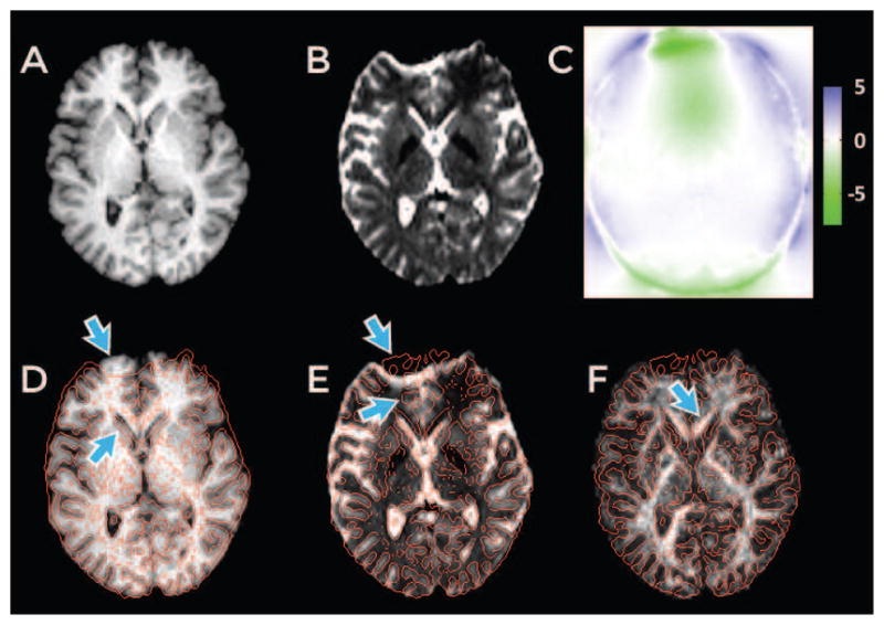
Example of distortion in a human brain T2W-EPI image acquired with EPI sequence. (A) An undistorted T1-weighted anatomical image. (B) T2W-EPI image from a diffusion dataset. (C) The displacement map (in millimeters) computed from an acquired fieldmap. Edges from the T2W-EPI image are overlaid in red on the T1-weighted image in (D) and vice-versa in (E) after rigid alignment (using INVERSION approach described later). Arrows point to areas with substantial distortion. (F) The fractional anisotropy (FA) map derived from diffusion dataset overlaid with edges from the T1-weighted image in red.

2.1. Inter-modal image registration

Image registration finds a spatial transformation of a moving image (I₁) which aligns it to a static image (I₂). The spatial transform is typically represented as a deformation map φ : X₂ → X₁ from the static image coordinate X₂ to moving image coordinate X₁. The optimal φ can be estimated by minimizing a cost-function of the form [ (I₂, I₁ ∘ φ) + α (φ)] where (·) measures dissimilarity between the images, I₁ ∘ φ is the transformed moving image such that (I₁ ∘ φ) (X₂) = I₁ (φ(X₂)), (·) is a regularization function that penalizes non-smooth deformation maps, and α is a regularization parameter [8, 9].

The choice of dissimilarity measure (·) is crucial for accurate registration of the images and it is desirable that (·) be sensitive to slight differences in alignment between the images. CR and MI are common dissimilarity measures that depend on the relationship between the distributions of the image intensities [30–32] and have been used widely in inter-modal registration [8–10]. However, both are non-convex and non-smooth over the transformation space which makes the cost-function difficult to minimize [8–10, 33–36]. INVERSION enables robust and consistent performance by making use of a smoother and simpler dissimilarity measure based on the sum of squared differences (SSD).

SSD is a simple dissimilarity measure between two images I₁ and I₂ expressed as [9]

$${\mathfrak{D}}_{\text{SSD}}(I_2,I_1)=\frac{1}{N_v}\sum _{\mathbf{X}\in \mathrm{\Omega }}{[I_2(\mathbf{X})-I_1(\mathbf{X})]}^2,$$ (1)

where Ω represents the set of voxels that are present in both the images and N_v is the cardinality of Ω. SSD is a well-behaved measure in images with similar contrast [9]. However, SSD is generally not appropriate for inter-modal registration problems [9, 50]. We use the INVERSION approach to first transform the contrast of the T2W-EPI image to look like that of the T1-weighted image (or vice versa) which allows us to exploit the nice properties of the SSD cost function.

2.2. INVERSION

INVERSION is motivated by the fact that both T1- and T2-weighted images from the same subject have similar anatomical structure but have an approximately inverted contrast relationship. Specifically, the image intensities are ordered such that white matter > gray matter > CSF in a T1-weighted anatomical image, while CSF > gray matter > white matter in a T2-weighted image. In the INVERSION method, we define the dissimilarity measure between T1-weighted anatomical image I_T1 and a corresponding T2W-EPI image I_EPI as 

$${\mathfrak{D}}_{\text{INV}}(I_{\text{EPI}},I_{\mathrm{T}1})={\mathfrak{D}}_{\text{SSD}}\left({\mathcal{F}}_{I_{\mathrm{T}1}}(I_{\text{EPI}}),I_{\mathrm{T}1}\right)+\beta {\mathfrak{D}}_{\text{SSD}}\left({\mathcal{F}}_{I_{\text{EP}1}}(I_{\mathrm{T}1}),I_{\text{EPI}}\right)$$ (2)

where (I_EPI) transforms the intensity of I_EPI to match the contrast of I_T1, (I_T1) transforms the intensity of I_T1 to match the contrast of I_EPI and β is a scalar weighting parameter determined experimentally. We assume, without loss of generality, that the intensities of both I_T1 and I_EPI are normalized to lie in the range [0,1] and express the first contrast matching transform as (I_EPI) = [f_IT1,IEPI(1 − I_EPI) · M_IEPI] where M_IEPI is a binary image representing the brain mask for the T2W-EPI image and f_IT1,_IEPI (·) is a monotonically increasing histogram matching function which is computed by matching the histograms of intensities inside the brain masks of the anatomical image I_T1 and the inverted T2W-EPI image (1 − I_EPI). (I_T1) is expressed in a similar fashion as (I_EPI) i.e. by interchanging I_T1 and I_EPI. We use histogram matching because both the T2W-EPI and T1-weighted image are acquired for the same subject and should depict the same tissues and tissue boundaries, but may differ in the intensities of each tissue. As a result, an intensity transformation should be able to approximately match the histogram of the images. We used our implementation of the histogram matching method described in [51] to estimate f_IT1,IEPI (·). In our studies, the brain masks are obtained by intensity thresholding of the T2W-EPI image and by using the BrainSuite software [52] for the T1-weighted image. An example of the INVERSION intensity transformation is shown in Fig. 2 for an in vivo dataset.

Figure 2.

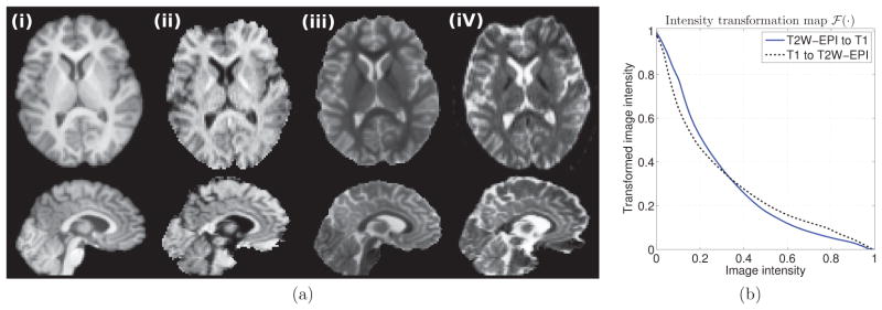
An example of INVERSION in an in vivo dataset. (a) shows corresponding slices from (i) the T1-weighted image, (ii) the intensity transformed T2W-EPI image, (iii) the intensity transformed T1-weighted image, and (iv) the original T2W-EPI image. (b) Intensity transformation maps (·) in INVERSION for voxels inside the brain mask for the dataset shown in (a).

Our registration-based distortion correction is initialized using a simple rigid alignment of the T2W-EPI and T1-weighted anatomical images (described in Section 2.2.1), which is followed by non-rigid registration to estimate the distortion (described in Section 2.2.2). Note that even if the DWIs have been distortion corrected using other methods, a rigid alignment is required for co-registration of the T1-weighted anatomical image and diffusion images. As a result, the rigid registration approach described in Section 2.2.1 is still useful in, e.g., cases where a B₀ fieldmap was acquired.

2.2.1. Rigid alignment using INVERSION

For rigid alignment, we set the T2W-EPI image (I_EPI) as the static image and we seek to estimate a rigid transformation φ_R1: X_EPI → X_T1 that maps the EPI coordinate X_EPI to the corresponding T1-weighted anatomical coordinate X_T1. The optimal rigid transformation φ_R1 is estimated by solving 

$${\widehat{\phi }}_{R_1}=\underset{{\phi }_{R_1}}{argmin}{\mathfrak{D}}_{\text{INV}}(I_{\text{EPI}},I_{\mathrm{T}1}\circ {\phi }_{R_1})$$ (3)

where I_T1 ∘ φ_R1 is the transformed T1-weighted anatomical image. The rigid transformation φ_R1 is parametrized by a vectors of six elements, representing translational and rotational components. Note that the contrast matching functions (·) and (·) are independent of rigid alignment and only need to be calculated once as a pre-computation before the actual registration process begins. In our experience, we found that the first contrast matching term in Eq. (2) is sufficient to obtain an accurate rigid alignment, so we set β = 0 in eq. (2) while solving Eq. (3), which also lowers the computational requirements.

We use a two step method to achieve robustness to local minima for large transformations while solving Eq. (3). Our first step involves a coarse grid search to quickly initialize with reasonable rotation parameters. Similar to other approaches [8–10], we use the centroids (center of mass) of each image to define the origins of their respective coordinate systems. Then we evaluate the registration cost function for each of several different rotations from a coarse grid defined over the three Euler angles. To enhance computational speed, this step is performed using low resolution images, which are generated by applying a Gaussian blur with a full-width at half-maximum (FWHM) of 5mm, followed by downsampling. For typical datasets (such as those shown in our results), this first stage requires 15–20 seconds to search over 2197 different rotations (stepsize of 15° over range of −90° to 90° for each Euler angle) on a modern 4-core 2.10GHz processor.

The second step applies a simple gradient descent approach to refine the registration parameters, initialized with the best rotation parameters found in the first step. We use numerically-computed gradients and a multi-resolution approach. Our two-step approach does not guarantee finding the globally-optimal solution, but is both fast and simple. In addition, our experience suggests that the well-behaved nature of the INVERSION cost function makes our approach robust to local minima and increases the chances of accurately aligning the images.

2.2.2. Distortion correction using INVERSION

Susceptibility-induced geometric distortions in diffusion MRI images are commonly modeled as being 1-dimensional as they occur primarily along the PED and are generally negligible along the readout and slice directions [11, 12, 23]. We can express the deformation due to B₀ inhomogeneity as a map φ_ΔB0: X_U → X_EPI which maps the coordinate X_U = (x_U, y_U, z_U) in an ideal undistorted image to the erroneous coordinate X_EPI = (x_EPI, y_EPI, z_EPI) in a distorted EPI image. Assuming that the PED is oriented along the y-axis, the ideal undistorted image I_U and distorted EPI image I_EPI are related as [11, 12, 20]

$$I_{\mathrm{U}}\approx \left|\frac{\partial y_{\text{EPI}}}{\partial y_{\mathrm{U}}}\right|\left(I_{\text{EPI}}\circ {\phi }_{\mathrm{\Delta }{B}_0}\right).$$ (4)

Further, ${\mathbf{X}}_{\text{EPI}}={\phi }_{\mathrm{\Delta }{B}_0}(x_{\mathrm{U}},y_{\mathrm{U}},z_{\mathrm{U}})=\left(x_{\mathrm{U}},y_{\mathrm{U}}+\frac{\gamma }{2\pi }\mathrm{\Delta }{B}_0(x_{\mathrm{U}},y_{\mathrm{U}},z_{\mathrm{U}})N\tau {\lambda }_y,z_{\mathrm{U}}\right)$ where ΔB₀ is the B₀ inhomogeneity (units of T), γ is the gyromagnetic ratio (2.675×10⁸ rad/s/T for protons), τ is the echo-spacing in seconds, N is the number of phase encoding steps in the EPI acquisition and λ_y is the spatial resolution of each voxel along the PED in appropriate units.

In the absence of a fieldmap, we estimate ΔB₀ by registering the distorted I_EPI to the undistorted anatomical image I_T1 in a non-rigid registration framework. This requires estimation of a non-rigid deformation map (φ_ΔB0) which would undistort I_EPI and a rigid transformation φ_R2: X_U → X_T1 which would align I_T1 to the undistorted image I_U. The optimal map is obtained by solving 

$$[{\widehat{\phi }}_{R_2};{\widehat{\phi }}_{\mathrm{\Delta }{B}_0}]=\underset{[{\phi }_{R_2};{\phi }_{\mathrm{\Delta }{B}_0}]}{argmin}\left[{\mathfrak{D}}_{\text{INV}}\left(\left|\frac{\partial y_{\text{EPI}}}{\partial y_{\mathrm{U}}}\right|\left(I_{\text{EPI}}\circ {\phi }_{\mathrm{\Delta }{B}_0}\right),I_{\mathrm{T}1}\circ {\phi }_{R_2}\right)+\alpha \mathcal{R}({\phi }_{\mathrm{\Delta }{B}_0})\right]$$ (5)

where is a regularizer explained later and α is a scalar weighting parameter determined experimentally. (·) is defined in eq. (2) with β equal to the ratio of mean intensities of I_T1 and I_EPI. In principle, we could have estimated a rigid transformation that maps the undistorted EPI image to the T1 image, instead of the other way around. The choice shown in Eq. (5) was motivated by computational efficiency. We parameterize φ_ΔB0 as the outer product of 1D cubic B-spline kernels with uniformly spaced control points and coefficients Φ_i,j,k corresponding to the (i, j, k)^th control point [53, 54]. In order to constrain the deformation along the PED, we only allow the y-coefficient of Φ_i,j,k to change while solving Eq. (5). We repeat and interpolate the end control points so that the deformation field is well-behaved everywhere, including along the boundary [53]. We use a regularizer that penalizes the roughness of the control-point coefficients as described in [55]. In our framework it is expressed as 

$$\mathcal{R}({\phi }_{\mathrm{\Delta }{B}_0})=\frac{1}{2}\sum _{i,j,k}\sum _{\mathbf{n}\in \mathcal{N}({\mathbf{\Phi }}_{i,j,k})}{\Vert {\mathbf{\Phi }}_{i,j,k}-{\mathbf{\Phi }}_{\mathbf{n}}\Vert }^2$$ (6)

where (Φ_i,j,k) is the set of control-points that are neighbors of Φ_i,j,k. This penalty encourages smoothness of the deformation field [55].

We solve Eq. (5) using a multi-resolution approach, which helps to avoid local minima and enables faster computation [8, 9]. Prior to solving Eq. (5), we rigidly align the T1-weighted image to the distorted T2W-EPI image using the method described in sec. 2.2.1. The contrast matching functions (·) and (·) depend on the estimate of φ_ΔB0 (as the intensities in the T2W-EPI image are modulated by the Jacobian of the transformation) and so they should, ideally, be updated at each iteration. However, we found that changes in the contrast matching function were negligible at each iteration and so we only compute once at the beginning of each level of the multi-resolution approach. In our implementation the B-spline control points are refined twice, starting from a separation of 28mm to final separation of 7mm, in a multi-resolution approach using the Lane-Riesenfeld Algorithm [56]. We use a simple gradient descent method for all the optimization and use analytical expressions for the gradients for efficient computation.

2.3. Materials

2.3.1. Experimental data

We evaluated the performance of the INVERSION method using simulated and multiple in vivo datasets. For simulations, we used images available from BrainWeb (http://brainweb.bic.mni.mcgill.ca/brainweb/) [57]. Although the BrainWeb phantom is artificially simple in contrast and image features, the availability of ground truth offers useful insight into the performance of the method. We used a simulated T2-weighted spin echo image (TR=10000m, TE=120ms, Flip angle=90°, 2mm slice thickness) as the undistorted T2W-EPI image and also simulated a corresponding T1-weighted MPRAGE image with 1mm isotropic resolution. To simulate EPI distortion, we used a real B₀ inhomogeneity map taken from an in vivo scan as ground truth distortion map and used a least-squares time segmentation approach to model the effects of field inhomogeneity on k-space data [58, 59]. We also added Gaussian noise to the modulus distorted image (in the image domain). The simulated distorted EPI image is shown in Fig. 7(b).

Figure 7.

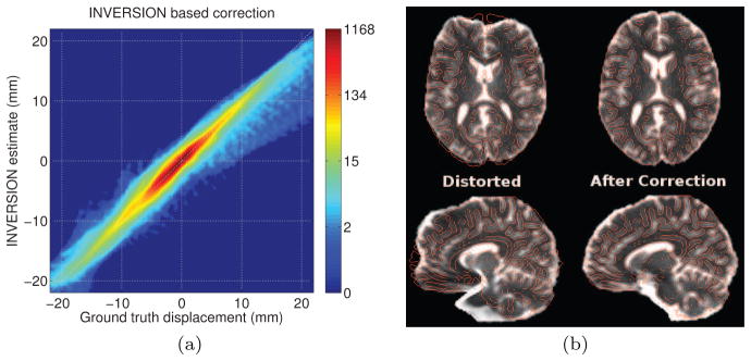
Performance of INVERSION-based distortion correction in the simulated BrainWeb dataset. The scatterplot of estimated displacement versus ground true displacement (calculated from the applied fieldmap) is shown as a joint histogram in (a). Note that the colorbars use a logarithmic scale to enhance visualization of the results for both minimally and severely distorted voxels. (b) Qualitative result of the INVERSION based correction in (top) an axial and (bottom) a sagittal slice. T2W-EPI images are overlaid with edge maps from the T1-weighted MPRAGE image in red.

We also evaluated performance using a total of 22 in vivo single-shot EPI diffusion brain scans. All scans were acquired on 3T scanners and B₀ fieldmaps were used as references to evaluate the registration-based deformation estimates. These 22 scans are divided into three different groups with different acquisition parameters, as summarized in Table 1. The differences in acquisition parameters ensures a more comprehensive evaluation of the proposed method.

Table 1.

Acquisition parameters for the in vivo datasets used for evaluation. The diffusion datasets differ mainly in echo spacing (ES), the use of parallel imaging, contrast parameters (TE, TR, and TI), b-values and resolution.

	Dataset-1	Dataset-2	Dataset-3
T1-weighted	TE=3.09ms, TR=2530ms	TE=3.09ms, TR=2530ms	TE=3.5ms, TR=2500ms
	TI=800ms, 1×1×1 mm3	TI=800ms, 1×1×1 mm3	TI=1200ms, 1×1×1 mm3
Diffusion	TE=88ms, TR=10000ms	TE=115ms, TR=10000ms	TE=85ms, TR=6000ms
	ES=0.85ms, 2×2×2 mm3	ES=0.69ms, 2×2×2 mm3	ES=0.81ms, 1.4×1.4×3.0 mm3
	b=1000s/mm2, GRAPPA 2×	b=2500s/mm2	b=1000s/mm2, GRAPPA 2×
B0 Fieldmap	TE1=10ms, TE2=12.46ms	TE1=10ms, TE2=12.46ms	TE1=4.92ms, TE2=7.38ms

Dataset-1 was a single-subject dataset, with the acquisition specifically designed to yield a good distortion-corrected reference image. Specifically, we used a specialized acquisition scheme for dataset-1 where we acquired each diffusion image with 4 different PEDs, which were combined to form a distortion-corrected reference image using the accurate 4-PED full method described in [17]. Datasets-2 and 3 represent typical diffusion images from ongoing neuroscience studies. Dataset-2 includes 10 subjects that were scanned at the University of Southern California under a grant to Hanna Damasio, PI, from the Air Force Office of Scientific Research (FA9620-10-1-109). Dataset-3 includes 11 subjects obtained from the NKI-Rockland sample [60].

2.3.2. Dissimilarity measures for evaluation

In our evaluation, we compare INVERSION against in-house implementations of normalized mutual information (NMI) and CR. For a pair of images I₁ and I₂, NMI is defined as [31]

$${\mathfrak{D}}_{\text{NMI}}(I_2,I_1)=\frac{H(I_1,I_2)}{H(I_1)+H(I_2)}$$ (7)

where H(I₁, I₂) = −Σ_i,j p(i, j) log p(i, j) is the standard joint entropy computed from joint intensity histogram p(i, j) of I₁ and I₂; and H(I₁) and H(I₂) are the marginal entropies computed similarly, but using the marginal histograms for I₁ and I₂ in place of the joint histogram. We used a Parzen window estimate [61] for all histograms and used only the intensities from voxels in the overlapping region of the two images. CR is defined as [32]

$${\mathfrak{D}}_{\text{CR}}(I_2,I_1)=\frac{{\sum }_{k=1}^K{N}_k\text{Var}(I_{2,k})}{N_v\text{Var}(I_2)}$$ (8)

where I_2,k = {I₂(ω); ω ∈ Ω_k}, ${\mathrm{\Omega }}_k=\{\omega \in \mathrm{\Omega };\frac{(k-1)}{K}\le I_1(\omega )<\frac{k}{K}\}$ is the k^th iso-set of I₁ in the image overlap region Ω, and N_v and N_k are the cardinalities of Ω and Ω_k respectively. In our implementation, we also used cost apodization for CR similar to that described in [36].

3. Results

3.1. Evaluation of dissimilarity measures

We studied the behavior of the different dissimilarity measures by observing how the different measures change when a T1-weighted image is misaligned from a corresponding co-registered T2W-EPI image. We used the accurate 4-PED full distortion corrected T2W-EPI image from dataset-1 for these experiments in order to avoid confounding factors due to distortion present in the diffusion datasets. To generate a gold standard co-registration, the T1-weighted image was rigidly registered to the T2W-EPI image using a manual procedure in Rview (http://rview.colin-studholme.net). The co-registered image pair was visually confirmed to have accurate alignment. Figure 3 illustrates the behavior of the different dissimilarity measures as we misalign the T1-weighted image by applying translation or rotation. Since multi-resolution approaches are commonly used for registration, this comparison is performed with several different degrees of Gaussian smoothing. Since CR is not a symmetric measure [32], i.e., (I₁, I₂) ≠ (I₂, I₁), we have plotted the two different versions of the CR measure that result from the two different possible choices of I₁. For the INVERSION measure, we use β = 0 in these experiments as both the terms in eq. (2) are based on SSD and we observed no improvement in performance by including the second term for rigid registration.

Figure 3.

Behavior of different dissimilarity measures as a function of misalignment by (a) translation along the x-axis and (b) rotation along the x-axis. Different lines represent different level of smoothing applied to both images and illustrate behavior at different resolutions. The full-width at half-maximum (FWHM) of the Gaussian smoothing is reported in units of millimeters (mm).

We show the behavior of misalignment with only translational components in Fig. 3(a) and with only rotational components in Fig. 3(b). The translation experiment (Fig. 3(a)) shows that the behavior of all cost functions is smooth when the Gaussian smoothing is large. Having a smooth cost function makes it easier to accurately solve the optimization problem, and helps justify the use of a multi-resolution approach. However, we observe that both the CR and NMI measures exhibit non-convex behavior when the translation is large. In contrast to CR and NMI, the INVERSION dissimilarity measure has a convex appearance even for large translational misalignment. The shape of this function suggests that it might be better-suited than CR and NMI for robustly finding the translational components.

The rotation experiment (Fig. 3(b)) shows similar behavior i.e. all cost functions are smooth when the Gaussian smoothing is large. However, all cost functions show non-convex behavior at large rotational misalignment and have local minima away from the globally-optimal solution for all levels of Gaussian smoothing. This means all the method could struggle to converge to the optimal solution using local optimization methods. This justifies our use of coarse grid search in Sec. 2.2.1 to find a good initialization with a limited number of cost evaluations. Fig. 3(b) shows that among all measures, the INVERSION measure has the widest area around the optimal solution which is well-behaved, especially for large Gaussian smoothing. This suggests that it has a higher chance of finding a good initial estimate in the coarse search over the rotation parameters and could avoid the need for multi-start optimization.

Expanding on our previous experiment, we next examined the characteristics of the different dissimilarity measures by performing rigid registration, without any initialization, of the T1-weighted and T2W-EPI images after applying known rigid transformations to the T1-weighted image. Specifically, we applied 96 known rigid transformations: 32 with only translation, 32 with only rotation and 32 with both translation and rotation. For each trial and each dissimilarity measure (NMI, CR, and INVERSION), a 6-parameter rigid registration was performed without any initialization and the residual root mean square (RMS) error in the rigid alignment was computed for each trial. The RMS errors were computed using the method described in [10, 62] where we represent the rigid transformations as 4×4 affine matrices. Specifically, for each applied (known) rigid transformation A, we obtain an estimated transformation  from the registration procedure. The RMS error in millimeters is then given by $d_{\text{RMS}}=\sqrt{\frac{1}{5}{a}^2\text{Tr}({\mathbf{M}}^{\top }\mathbf{M})+{\mathbf{t}}^{\top }\mathbf{t}}$ where a is the radius of the brain region (with a spherical approximation), while M is a 3×3 matrix and t is a column vector of length 3 computed according to $\left[\begin{array}{cc}\mathbf{M}& \mathbf{t}\\ 000& 0\end{array}\right]={\widehat{\mathbf{A}}}^{-1}\mathbf{A}-\mathbf{I}$. For CR based registration, we used the T2W-EPI image as I₁, since as suggested by Fig. 3, this leads to a better-behaved cost function and higher accuracy.

The results of this evaluation are shown in Fig. 4. In the absence of any initialization, the CR and NMI based methods perform well for small misalignments (approximately less than 10 mm) but perform poorly when the misalignment is large. This observation is consistent with the relatively flat behavior of these measures and presence of local minima that was observed in Fig. 3. In contrast, the INVERSION method consistently showed good performance across all transformations and was robust to large transformation even without any initialization. This demonstrates the well-behaved nature of INVERSION over a wider region around the optimal solution. However, it should be noticed that whenever the NMI based measure performed well, it showed lowest error among all the measures. This could probably be explained by the fact that it makes the fewest assumptions about the different images, and is therefore the least sensitive to assumption violations. This motivated us to use the NMI based registration as a refinement step after INVERSION in our software implementation. Fig. 5 shows a result of such refinement (note that all other results presented in this paper do not use any NMI-based refinement). It can be noticed that most edges are well aligned with sulci and gyri after INVERSION and the NMI-based refinement adds a very subtle improvement.

Figure 4.

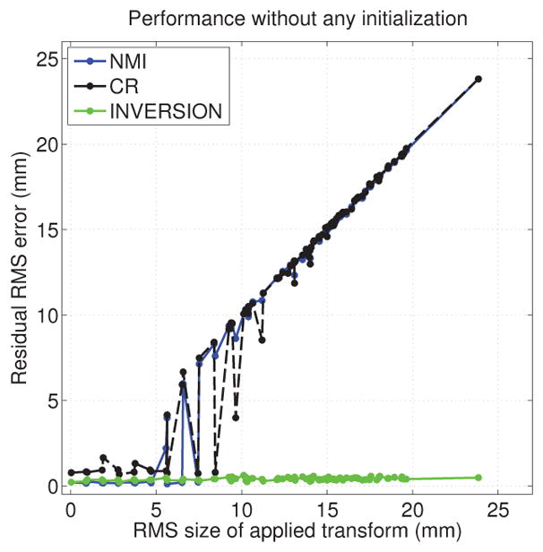
Performance of different dissimilarity measures as a function of the applied transformation in a rigid registration experiment without any initialization.

3.2. Comparison with existing methods for rigid-alignment

We also compared INVERSION to two registration methods provided in the FMRIB Software Library (FSL) [13] in a rigid registration experiment similar to that described in the previous section. We used the default settings with 6 degrees of freedom on FMRIB’s Linear Image Registration Tool (FLIRT version 6.0) as the first method which uses a CR-based cost function in a hybrid global-local optimization approach for inter-modal rigid-registration [10, 36]. For the second method we used EPI-Reg (http://fsl.fmrib.ox.ac.uk/fsl/fslwiki/FLIRT/UserGuide#epi_reg) which uses a boundary-based cost function [63] along with FLIRT’s global-local optimization approach. These two methods were selected for comparison because FLIRT is widely used for affine registration by brain-mapping community and because EPI-Reg is specifically designed for registration of EPI images to anatomical (e.g. T1-weighted) images. We applied 194 known (randomly generated) rigid transformations to the pre-registered T1-weighted MPRAGE image from the previous section and used all the methods to estimate the rigid deformation. We used the accurate 4-PED full distortion corrected T2W-EPI image from dataset-1 as the static image for all the methods to avoid confounding factors due to distortion. Fig. 6(a) and (b) compares the performance of different methods in this experiment. The results show that all the three methods show low RMS error across all applied transformations. EPI-Reg performs better than FLIRT in most cases, which is expected as EPI-Reg is specifically tailored for registration with EPI images and uses a sophisticated tissue classification for boundary-based cost function. The proposed INVERSION method shows consistent behavior and the lowest RMS error for most of the applied transformation. Fig. 6(b) summarizes of the performance across all the applied transformation and indicates that the INVERSION based method outperforms all the other methods in this comparison.

Figure 6.

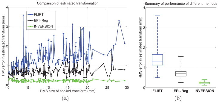
(a) Comparison of INVERSION to existing methods in a rigid registration experiment. (b) Box-and-whisker plot showing the summary of performance of different methods. The line inside the box represents the median RMS error and the whiskers extend to minimum and maximum RMS error.

3.3. Evaluation of INVERSION-based distortion correction

We first evaluated the proposed distortion correction method using the BrainWeb simulation data, comparing the distortion field estimated by INVERSION with the ground truth B₀ inhomogeneity map. Fig. 7(a) shows this comparison as a joint-histogram, which was computed using a Parzen-window estimate of the binned voxel counts. For ideal distortion correction, the joint histogram should be concentrated along the 45° line where the estimated distortion is equal to the true distortion. As seen in Fig. 7(a) our distortion estimate closely follows the ground truth. The mean absolute error in the displacement estimate was 0.8 ± 1.4 mm inside the brain mask. Fig. 7(b) shows a qualitative result of the corrected T2W-EPI images with edge maps from the anatomical image overlaid in red. It can be noticed that edges align well with sulci and gyri accurately after INVERSION based distortion correction.

Next, we evaluated the performance of the proposed registration-based distortion correction method using several in vivo datasets. We measured performance by comparing the INVERSION displacement field against that from the corresponding fieldmap. We also compared the performance of the proposed method to that of a NMI-based distortion correction method, described in [23]. A MI-based method was used for this comparison because it has been used for EPI distortion correction in several previous approaches [20, 23–25, 27, 28] and because MI-based methods are widely used for inter-modal registration [8, 9, 30, 31]. We present the results using the two methods for dataset-1 in Fig. 8. Fig. 8(a) shows the joint-histogram of the displacement estimates and the reference inside the brain-mask. As seen in the figure, the NMI-based method performs well for small distortions, but has large deviations from the 45° line for larger distortions. In contrast, the joint histogram for the INVERSION method is more concentrated around the 45° line indicating overall better estimation of distortion field in most areas. Fig. 8(b) summarizes the performance of both the methods across all the voxels. For easier comparison we divide all the voxels in two sets, one set with minimal distortion (less than 2mm of reference displacement) and the other with severe distortion (more than 2mm of reference displacement). The INVERSION approach shows overall lower absolute error in the displacement estimates for all the voxels as compared to NMI-based distortion correction. Fig. 8(c) shows a qualitative comparison of the corrected T2W-EPI images with edge maps from the anatomical image overlaid in red. We also show the corrected T2W-EPI images using the acquired fieldmap for reference. From the overlay images, it can be noticed that both the registration-based methods show similar alignment of anatomical structures, however there are some differences. The NMI based correction shows poorer performance in areas with severe distortion as can be seen in frontal and occipital areas of the brain. The INVERSION based distortion correction shows better correspondence than NMI to the reference correction, as seen in regions indicated by arrows. Fig. 8(d) shows absolute errors in the displacement estimates as compared to that calculated from the fieldmap. The NMI based method shows larger errors around air-tissue boundaries, especially in frontal areas of the brain, while INVERSION based correction shows overall lower errors in all areas.

Figure 8.

Performance of registration-based distortion correction in dataset-1. (a) The joint-histogram of the reference displacement (calculated from the fieldmap) and estimated displacement using (left) NMI and (right) INVERSION based method. (b) Box-and-whisker plots showing the absolute error in displacement estimated using NMI and INVERSION based distortion correction methods across (left) minimally distorted and (right) severely distorted voxels. The box extends from 25^th to 75^th percentile with the interior line representing the median and the whiskers extending from 10^th to 90^th percentile. (c) Qualitative comparison of distortion correction methods in (top) an axial and (bottom) a sagittal slice. Fieldmap based correction is shown as a reference for comparison. The distortion-corrected T2W-EPI images are shown overlaid with edge maps from the T1-weighted MPRAGE image in red. Arrows point to areas with inaccurate distortion correction in the NMI-based correction. (d) Visualization of the absolute errors (in mm) in displacement relative to the fieldmap estimated by INVERSION and NMI-based methods in (top) an axial and (bottom) a sagittal slice.

Next we compared the performance of INVERSION and NMI relative to the measured fieldmap using 21 scans from datasets-2 and 3. Fig. 9(a) shows the pooled joint-histogram of displacement estimates and reference displacement values for all subjects. Similar to previous observations, the joint histogram for the INVERSION method follows the 45° line indicating overall better estimation of distortion as compared to NMI-based method. Fig. 9(b) shows the histogram of absolute errors in the displacement estimates as compared to the fieldmap displacement for minimally and severely distorted voxels. Both registration methods show good and similar performance for minimal distortion. However, the NMI-based method had substantial error for severely distorted voxels. A summary of performance of both the method for individual subjects is shown in Fig. 9(c) for severely distorted voxels (performance was similar for both the methods for minimally distorted voxels). Of the two methods, INVERSION shows lower median error and lower range of absolute errors for all subjects. Runtimes for the INVERSION-based approach were in the range of 6–15 minutes for all subjects, while the NMI-based method had runtimes from 10–30 minutes. Both methods were implemented in MATLAB on a 4-core 2.10GHz processor.

Figure 9.

Performance of registration-based distortion correction with 21 subjects from dataset-2 and 3. (a) The pooled joint-histogram of the reference displacement (calculated from the fieldmap) and estimated displacement using (left) NMI and (right) INVERSION based methods for all subjects. Note that the colorbars use a logarithmic scale. (b) Histogram of the absolute errors in displacement estimate for (left) minimally and (right) severely distorted voxels. (c) Box-and-whisker plot showing the absolute error in the displacement estimated in severely distorted areas for each subject using NMI and INVERSION based distortion correction method. The box extends from 25^th to75^th percentile with the dot inside the box representing the median error and the whiskers extend from 10^th to 90^th percentile. Subjects from dataset-2 have labels starting with ‘N’ and subjects from dataset-3 have labels starting with ‘A’.

4. Discussion

Our results demonstrate that INVERSION can accurately co-register diffusion MRI and T1-weighted anatomical images. INVERSION improves the robustness of co-registration by using the simpler and smoother SSD dissimilarity measure by exploiting the approximately inverted contrast relationship in T2- and T1-weighted images of the human brain. This approach could also be applied to other multi-modal registration problems with similar contrast relationships.

It should be noted that more accurate correction of distorted EPI images can be performed in the presence of a fieldmap and/or more advanced acquisition schemes [6, 11–19]. Hence, we recommend the use of these approaches when they are available. However, even in such cases, INVERSION can still be useful for rigid alignment of the diffusion images to the T1-weighted anatomical image.

The intensity transformation used by INVERSION is only approximate, and this is especially true in regions with partial voluming between different tissue types. This is evident when looking at the boundaries between the white matter and the ventricles in Fig. 2. This difference is caused by both mismatched resolution and the fact that INVERSION should ideally be applied to white matter and cerebrospinal fluid separately when both are present within the same voxel (the inverse of the sum is not the same as the sum of the inverses). For rigid transformations, the low dimensionality of the transform appears to provide some level of robustness against this problem so that the final registration errors are small as shown in Fig. 6. For nonrigid transformations, we found that the symmetric measure, where we map intensities from T1 to EPI as well as from EPI to T1, reduces sensitivity to this effect producing improved results relative to mapping in only one direction.

INVERSION uses a coarse search for initialization of rotation parameters followed by a local optimization strategy to solve Eq. (3), which does not guarantee to find the optimally-global solution. Multi-start hybrid global-local optimization approaches [10, 36] could be used in place of our search-based initialization scheme. However, as shown in the results section, the smoothness of our dissimilarity measure makes the search-based initialization followed by local optimization robust to local minima.

Use of INVERSION requires a background segmentation as the background does not contribute any MR signal and should appear dark in both the diffusion and anatomical images. This pre-processing step is straightforward for most images with reasonable SNR, as the background can be easily detected based on intensity thresholding.

Another factor which can limit the use of INVERSION are images with inhomogeneous intensities resulting from bias fields, severe susceptibility-induced distortion, and other related sources. Bias fields are uncorrected intensity nonuniformities that can have a variety of causes [64, 65]. In case one of the images suffers from a severe bias field, the inverted contrast relationship may no longer be a reasonable approximation. However the confounding effects of bias field are not limited to the INVERSION approach, and other dissimilarity measures based on MI and CR will also have similar problems resulting from bias fields. Our acquired in vivo data had minor bias fields, but we did not notice any issues with INVERSION. In principle, bias field correction software [52, 66] can be applied in cases where the scanner produces images with severe bias fields.

Similarly, areas affected by severe susceptibility-induced distortion may not follow the inverted contrast relationship, since susceptibility-induced distortion can change local tissue intensities. It is possible that severely distorted voxels may bias results when they are included in estimation of the contrast matching function. In order to reduce the effects of these severe intensity distortions, the contrast matching function could be estimated at each iteration while solving Eq. (5). Another approach could be to identify the severely distorted voxels and exclude them from the estimation of the contrast matching function. However, in our experience, the number of highly distorted voxels was small compared to the number of minimally distorted voxels in our images and the estimation of the histogram-matching function did not change substantially because of these voxels.

5. Conclusion

We described a new method for the correction of susceptibility-induced distortion in diffusion images and the co-registration of diffusion images with T1-weighted anatomical images. Our method combines an appropriate mathematical model based on the physics of distortion in EPI images, with prior information about the contrast relationships between T1 and T2-weighted brain images. Evaluations of our method with in vivo datasets demonstrate improved distortion correction relative to normalized mutual information in diffusion weighted images in the absence of a fieldmap and robust alignment with T1-weighted anatomical images. Our methods are implemented in a freely available software (http://brainsuite.org/).

Highlights.

• We describe INVERSION, a new method for rigid coregistration of diffusion and structural (T1-weighted) images.

• The known contrast relationship between these image types is exploited to obtain a smoother cost function.

• INVERSION can also be used for distortion correction of diffusion images without a fieldmap

• INVERSION rigidly-aligns image more accurately than current software tools/methods against which we compared.

• Our method also achieves lower errors for distortion correction than normalized mutual information.

References

- 1.Le Bihan D, Johansen-Berg H. Diffusion MRI at 25: Exploring brain tissue structure and function. NeuroImage. 2012;61(2):324–341. doi: 10.1016/j.neuroimage.2011.11.006. [DOI] [PMC free article] [PubMed] [Google Scholar]
- 2.Johansen-Berg H, Behrens TE. Diffusion MRI: from Quantitative Measurement to in-vivo Neuroanatomy. Academic Press; San Diego: 2009. [Google Scholar]
- 3.Jones DK. Diffusion MRI: Theory, Methods, and Applications. Oxford University Press; New York: 2011. [Google Scholar]
- 4.Jones DK, Cercignani M. Twenty-five pitfalls in the analysis of diffusion MRI data. NMR in Biomedicine. 2010;23(7):803–820. doi: 10.1002/nbm.1543. [DOI] [PubMed] [Google Scholar]
- 5.Irfanoglu MO, Walker L, Sarlls J, Marenco S, Pierpaoli C. Effects of image distortions originating from susceptibility variations and concomitant fields on diffusion MRI tractography results. NeuroImage. 2012;61(1):275–288. doi: 10.1016/j.neuroimage.2012.02.054. [DOI] [PMC free article] [PubMed] [Google Scholar]
- 6.Andersson JLR, Skare S. Image Distortion and Its Correction in Diffusion MRI. In: Jones DK, editor. Diffusion MRI: Theory, Methods, and Applications. Oxford University Press; USA: 2011. pp. 285–302. [DOI] [Google Scholar]
- 7.Jezzard P, Clare S. Sources of distortion in functional MRI data. Human Brain Mapping. 1999;8(2–3):80–85. doi: 10.1002/(SICI)1097-0193(1999)8:2/3<80::AID-HBM2>3.0.CO;2-C. [DOI] [PMC free article] [PubMed] [Google Scholar]
- 8.Oliveira FPM, ao Manuel J, Tavares RS. Medical image registration: a review. Computer Methods in Biomechanics and Biomedical Engineering. 2012;0(0):1–21. doi: 10.1080/10255842.2012.670855. [DOI] [PubMed] [Google Scholar]
- 9.Derek MH, Hill LG, Batchelor Philipp G, Hawkes DJ. Medical image registration. Physics in Medicine and Biology. 2001;46(3):R1–R45. doi: 10.1088/0031-9155/46/3/201. [DOI] [PubMed] [Google Scholar]
- 10.Jenkinson M, Smith S. A global optimisation method for robust affine registration of brain images. Medical Image Analysis. 2001;5(2):143–156. doi: 10.1016/S1361-8415(01)00036-6. [DOI] [PubMed] [Google Scholar]
- 11.Jezzard P, Balaban RS. Correction for geometric distortion in echo planar images from B0 field variations. Magnetic Resonance in Medicine. 1995;34(1):65–73. doi: 10.1002/mrm.1910340111. [DOI] [PubMed] [Google Scholar]
- 12.Jezzard P. Correction of geometric distortion in fMRI data. NeuroImage. 2012;62(2):648–651. doi: 10.1016/j.neuroimage.2011.09.010. [DOI] [PubMed] [Google Scholar]
- 13.Jenkinson M, Beckmann CF, Behrens TE, Woolrich MW, Smith SM. FSL. NeuroImage. 2012;62(2):782–790. doi: 10.1016/j.neuroimage.2011.09.015. [DOI] [PubMed] [Google Scholar]
- 14.Munger P, Crelier GR, Peters TM, Pike GB. An inverse problem approach to the correction of distortion in EPI images. IEEE Transactions on Medical Imaging. 2000;19(7):681–689. doi: 10.1109/42.875186. [DOI] [PubMed] [Google Scholar]
- 15.Kadah YM, Hu X. Algebraic reconstruction for magnetic resonance imaging under B0 inhomogeneity. IEEE Transactions on Medical Imaging. 1998;17(3):362–370. doi: 10.1109/42.712126. [DOI] [PubMed] [Google Scholar]
- 16.Bhushan C, Joshi AA, Leahy RM, Haldar JP. Accelerating Data Acquisition for Reversed-Gradient Distortion Correction in Diffusion MRI: A Constrained Reconstruction Approach. 21st Scientific Meeting of International Society for Magnetic Resonance in Medicine (ISMRM); Salt Lake City, Utah. 2013. p. 55. [Google Scholar]
- 17.Bhushan C, Joshi AA, Leahy RM, Haldar JP. Improved B0-distortion correction in diffusion MRI using interlaced q-space sampling and constrained reconstruction. Magnetic Resonance in Medicine. doi: 10.1002/mrm.25026. [DOI] [PMC free article] [PubMed] [Google Scholar]
- 18.Andersson JLR, Skare S, Ashburner J. How to correct susceptibility distortions in spin-echo echo-planar images: application to diffusion tensor imaging. NeuroImage. 2003;20(2):870–888. doi: 10.1016/S1053-8119(03)00336-7. [DOI] [PubMed] [Google Scholar]
- 19.Gallichan D, Andersson JLR, Jenkinson M, Robson MD, Miller KL. Reducing distortions in diffusion-weighted echo planar imaging with a dual-echo blip-reversed sequence. Magnetic Resonance in Medicine. 2010;64(2):382–390. doi: 10.1002/mrm.22318. [DOI] [PubMed] [Google Scholar]
- 20.Studholme C, Constable RT, Duncan JS. Accurate alignment of functional EPI data to anatomical MRI using a physics-based distortion model. IEEE Transactions on Medical Imaging. 2000;19(11):1115–1127. doi: 10.1109/42.896788. [DOI] [PubMed] [Google Scholar]
- 21.Kybic J, Thévenaz P, Nirkko A, Unser M. Unwarping of unidirectionally distorted EPI images. IEEE Transactions on Medical Imaging. 2000;19(2):80–93. doi: 10.1109/42.836368. [DOI] [PubMed] [Google Scholar]
- 22.Ardekani S, Sinha U. Geometric distortion correction of high-resolution 3 T diffusion tensor brain images. Magnetic Resonance in Medicine. 2005;54(5):1163–1171. doi: 10.1002/mrm.20651. [DOI] [PubMed] [Google Scholar]
- 23.Bhushan C, Haldar JP, Joshi AA, Leahy RM. Correcting Susceptibility-Induced Distortion in Diffusion-Weighted MRI using Constrained Nonrigid Registration. Asia-Pacific Signal Information Processing Association Annual Summit and Conference (APSIPA ASC); Hollywood, CA. 2012. pp. 1–9. [PMC free article] [PubMed] [Google Scholar]
- 24.Pierpaoli C, Walker L, Irfanoglu MO, Barnett A, Basser P, Chang L, Koay C, Pajevic S, Rohde G, Sarlls J, Wu M. TORTOISE: an integrated software package for processing of diffusion MRI data. International Society for Magnetic Resonance in Medicine; Stockholm, Sweden. 2010. p. 1597. [Google Scholar]
- 25.Wu M, Chang L-C, Walker L, Lemaitre H, Barnett A, Marenco S, Pierpaoli C. Comparison of EPI Distortion Correction Methods in Diffusion Tensor MRI Using a Novel Framework. In: Metaxas D, Axel L, Fichtinger G, Székely G, editors. Medical Image Computing and Computer-Assisted Intervention – MICCAI 2008, vol. 5242 of Lecture Notes in Computer Science. Springer; Berlin / Heidelberg: 2008. pp. 321–329. [DOI] [PMC free article] [PubMed] [Google Scholar]
- 26.Huang H, Ceritoglu C, Li X, Qiu A, Miller MI, van Zijl PC, Mori S. Correction of B0 susceptibility induced distortion in diffusion-weighted images using large-deformation diffeomorphic metric mapping. Magnetic Resonance Imaging. 2008;26(9):1294–1302. doi: 10.1016/j.mri.2008.03.005. [DOI] [PMC free article] [PubMed] [Google Scholar]
- 27.Gholipour A, Kehtarnavaz N, Gopinath K, Briggs R, Devous M, Haley R. Distortion Correction via Non-rigid Registration of Functional to Anatomical Magnetic Resonance Brain Images. IEEE International Conference on Image Processing; 2006. pp. 1181–1184. [DOI] [Google Scholar]
- 28.Yao X-F, Song Z-J. Deformable Registration for Geometric Distortion Correction of Diffusion Tensor Imaging. In: Real P, Diaz-Pernil D, Molina-Abril H, Berciano A, Kropatsch W, editors. Computer Analysis of Images and Patterns, vol. 6854 of Lecture Notes in Computer Science. Springer; Berlin / Heidelberg: 2011. pp. 545–553. [Google Scholar]
- 29.Maes F, Collignon A, Vandermeulen D, Marchal G, Suetens P. Multimodality image registration by maximization of mutual information, Medical Imaging. IEEE Transactions on. 1997;16(2):187–198. doi: 10.1109/42.563664. [DOI] [PubMed] [Google Scholar]
- 30.Viola P, Wells WM., III Alignment by Maximization of Mutual Information. International Journal of Computer Vision. 1997;24(2):137–154. doi: 10.1023/A:1007958904918. [DOI] [Google Scholar]
- 31.Studholme C, Hill D, Hawkes DJ. An overlap invariant entropy measure of 3D medical image alignment. Pattern Recognition. 1999;32(1):71–86. doi: 10.1016/S0031-3203(98)00091-0. [DOI] [Google Scholar]
- 32.Roche A, Malandain G, Pennec X, Ayache N. The correlation ratio as a new similarity measure for multimodal image registration. In: Wells W, Colchester A, Delp S, editors. Medical Image Computing and Computer-Assisted Interventation – MICCAI’98, vol. 1496 of Lecture Notes in Computer Science. Springer; Berlin Heidelberg: 1998. pp. 1115–1124. [DOI] [Google Scholar]
- 33.Pluim JP, Maintz JA, Viergever MA. Mutual-information-based registration of medical images: a survey. IEEE Transactions on Medical Imaging. 2003;22(8):986–1004. doi: 10.1109/TMI.2003.815867. [DOI] [PubMed] [Google Scholar]
- 34.Tsao J. Interpolation artifacts in multimodality image registration based on maximization of mutual information. IEEE Transactions on Medical Imaging. 2003;22(7):854–864. doi: 10.1109/TMI.2003.815077. [DOI] [PubMed] [Google Scholar]
- 35.Pluim JP, Maintz JBA, Viergever MA. f -information measures in medical image registration, Medical Imaging. IEEE Transactions on. 2004;23(12):1508–1516. doi: 10.1109/TMI.2004.836872. [DOI] [PubMed] [Google Scholar]
- 36.Jenkinson M, Bannister P, Brady M, Smith S. Improved Optimization for the Robust and Accurate Linear Registration and Motion Correction of Brain Images. NeuroImage. 2002;17(2):825–841. doi: 10.1006/nimg.2002.1132. [DOI] [PubMed] [Google Scholar]
- 37.Pierpaoli C. Artifacts in Diffusion MRI. In: Jones DK, editor. Diffusion MRI: Theory, Methods, and Applications. 2010. pp. 303–317. [Google Scholar]
- 38.Friston KJ, Ashburner J, Frith CD, Poline JB, Heather JD, Frackowiak RSJ. Spatial registration and normalization of images. Human Brain Mapping. 1995;3(3):165–189. doi: 10.1002/hbm.460030303. [DOI] [Google Scholar]
- 39.Mercier L, Fonov V, Haegelen C, Del Maestro R, Petrecca K, Collins D. Comparing two approaches to rigid registration of three-dimensional ultrasound and magnetic resonance images for neurosurgery. International Journal of Computer Assisted Radiology and Surgery. 2012;7(1):125–136. doi: 10.1007/s11548-011-0620-2. [DOI] [PubMed] [Google Scholar]
- 40.Choi K, Franco AR, Holtzheimer PE, Mayberg HS, Hu XP. Diffusion tensor imaging distortion correction with T1. International Society for Magnetic Resonance in Medicine (ISMRM); Montréal, Québec, Canada. 1946; 2011. [Google Scholar]
- 41.Miller MI, Christensen GE, Amit Y, Grenander U. Mathematical textbook of deformable neuroanatomies. Proceedings of the National Academy of Sciences. 1993;90(24):11944–11948. doi: 10.1073/pnas.90.24.11944. [DOI] [PMC free article] [PubMed] [Google Scholar]
- 42.Roy S, Carass A, Prince JL. Magnetic Resonance Image Example-Based Contrast Synthesis. IEEE Transactions on Medical Imaging. 2013;32(12):2348–2363. doi: 10.1109/TMI.2013.2282126. [DOI] [PMC free article] [PubMed] [Google Scholar]
- 43.Meyer J. Histogram Transformation for Inter-Modality Image Registration. Proceedings of the 7th IEEE International Conference on Bioinformatics and Bioengineering; 2007. pp. 1118–1123. [DOI] [Google Scholar]
- 44.Kroon D-J, Slump CH. MRI modalitiy transformation in demon registration. IEEE International Symposium on Biomedical Imaging: From Nano to Macro; 2009. pp. 963–966. [DOI] [Google Scholar]
- 45.Guimond A, Roche A, Ayache N, Meunier J. Three-dimensional multimodal brain warping using the Demons algorithm and adaptive intensity corrections. IEEE Transactions on Medical Imaging. 2001;20(1):58–69. doi: 10.1109/42.906425. [DOI] [PubMed] [Google Scholar]
- 46.Chang H, Fitzpatrick JM. A technique for accurate magnetic resonance imaging in the presence of field inhomogeneities. IEEE Transactions on Medical Imaging. 1992;11(3):319–329. doi: 10.1109/42.158935. [DOI] [PubMed] [Google Scholar]
- 47.Bowtell R, McIntyre D, Commandre M, Glover P, Mansfield P. Correction of geometric distortion in echo planar images. Proceedings of the Society of Magnetic Resonance; San Francisco. 1994. p. 411. [Google Scholar]
- 48.Morgan PS, Bowtell RW, McIntyre DJ, Worthington BS. Correction of spatial distortion in EPI due to inhomogeneous static magnetic fields using the reversed gradient method. Journal of Magnetic Resonance Imaging. 2004;19(4):499–507. doi: 10.1002/jmri.20032. [DOI] [PubMed] [Google Scholar]
- 49.Holland D, Kuperman JM, Dale AM. Efficient correction of inhomogeneous static magnetic field-induced distortion in Echo Planar Imaging. NeuroImage. 2010;50(1):175–183. doi: 10.1016/j.neuroimage.2009.11.044. [DOI] [PMC free article] [PubMed] [Google Scholar]
- 50.Viola PA. PhD thesis. Massachusetts Institute of Technology; 1995. Alignment by Maximization of Mutual Information. [Google Scholar]
- 51.Gonzalez RC, Woods RE. Digital Image Processing. Prentice-Hall Inc; Upper Saddle River, New Jersey: 2002. [Google Scholar]
- 52.Shattuck DW, Sandor-Leahy SR, Schaper KA, Rottenberg DA, Leahy RM. Magnetic Resonance Image Tissue Classification Using a Partial Volume Model. NeuroImage. 2001;13(5):856–876. doi: 10.1006/nimg.2000.0730. [DOI] [PubMed] [Google Scholar]
- 53.Bartels RH, Beatty JC, Barsky BA. An Introduction to Splines for Use in Computer Graphics & Geometric Modeling. Morgan Kaufmann Publishers Inc; San Francisco, CA, USA: 1987. [Google Scholar]
- 54.Rueckert D, Sonoda L, Hayes C, Hill D, Leach M, Hawkes D. Nonrigid registration using free-form deformations: application to breast MR images. IEEE Transactions on Medical Imaging. 1999;18(8):712–721. doi: 10.1109/42.796284. [DOI] [PubMed] [Google Scholar]
- 55.Chun SY, Fessler JA. A Simple Regularizer for B-spline Nonrigid Image Registration That Encourages Local Invertibility. IEEE Journal of Selected Topics in Signal Processing. 2009;3(1):159–169. doi: 10.1109/JSTSP.2008.2011116. [DOI] [PMC free article] [PubMed] [Google Scholar]
- 56.Lane JM, Riesenfeld RF. A Theoretical Development for the Computer Generation and Display of Piecewise Polynomial Surfaces. IEEE Transactions on Pattern Analysis and Machine Intelligence. 1980;PAMI-2(1):35–46. doi: 10.1109/TPAMI.1980.4766968. [DOI] [PubMed] [Google Scholar]
- 57.Cocosco CA, Kollokian V, Kwan RK-S, Pike GB, Evans AC. BrainWeb: Online interface to a 3D MRI simulated brain database. NeuroImage, Proceedings of 3rd International Conference on Functional Mapping of the Human Brain; Copenhagen. Citeseer; 1997. p. S425. [Google Scholar]
- 58.Sutton BP, Noll DC, Fessler JA. Fast, iterative image reconstruction for MRI in the presence of field inhomogeneities. IEEE Transactions on Medical Imaging. 2003;22(2):178–188. doi: 10.1109/TMI.2002.808360. [DOI] [PubMed] [Google Scholar]
- 59.Gai J, Obeid N, Holtrop JL, Wu X-L, Lam F, Fu M, Haldar JP, mei W, Hwu W, Liang Z-P, Sutton BP. More IMPATIENT: A gridding-accelerated Toeplitz-based strategy for non-Cartesian high-resolution 3D MRI on GPUs. Journal of Parallel and Distributed Computing. 2013;73(5):686–697. doi: 10.1016/j.jpdc.2013.01.001. [DOI] [PMC free article] [PubMed] [Google Scholar]
- 60.Nooner KB, Colcombe S, Tobe R, Mennes M, Benedict M, Moreno A, Panek L, Brown S, Zavitz S, Li Q, Sikka S, Gutman D, Bangaru S, Schlachter RT, Kamiel S, Anwar A, Hinz C, Kaplan M, Rachlin A, Adelsberg S, Cheung B, Khanuja R, Yan C, Craddock C, Calhoun V, Courtney W, King M, Wood D, Cox C, Kelly C, DiMartino A, Petkova E, Reiss P, Duan N, Thompsen D, Biswal B, Coffey B, Hoptman M, Javitt DC, Pomara N, Sidtis J, Koplewicz H, Castellanos FX, Leventhal B, Milham M. The NKI-Rockland Sample: A Model for Accelerating the Pace of Discovery Science in Psychiatry. Frontiers in Neuroscience. 6:152. doi: 10.3389/fnins.2012.00152. [DOI] [PMC free article] [PubMed] [Google Scholar]
- 61.Duda RO, Hart PE, Stork DG. Pattern Classification. Vol. 10. John Wiley and Sons, Inc; New York: 2001. [Google Scholar]
- 62.Jenkinson M. Tech Rep. Oxford Centre for Functional Magnetic Resonance Imaging of the Brain, Department of Clinical Neurology, Oxford University; Oxford, UK: 2000. Measuring transformation error by RMS deviation. [Google Scholar]
- 63.Greve DN, Fischl B. Accurate and robust brain image alignment using boundary-based registration. NeuroImage. 2009;48(1):63–72. doi: 10.1016/j.neuroimage.2009.06.060. [DOI] [PMC free article] [PubMed] [Google Scholar]
- 64.Sled JG, Pike GB. Standing-wave and RF penetration artifacts caused by elliptic geometry: an electrodynamic analysis of MRI. IEEE Transactions on Medical Imaging. 1998;17(4):653–662. doi: 10.1109/42.730409. [DOI] [PubMed] [Google Scholar]
- 65.Simmons A, Tofts PS, Barker GJ, Arridge SR. Sources of intensity nonuniformity in spin echo images at 1.5 T. Magnetic Resonance in Medicine. 1994;32(1):121–128. doi: 10.1002/mrm.1910320117. [DOI] [PubMed] [Google Scholar]
- 66.Sled JG, Zijdenbos AP, Evans AC. A nonparametric method for automatic correction of intensity nonuniformity in MRI data. IEEE Transactions on Medical Imaging. 1998;17(1):87–97. doi: 10.1109/42.668698. [DOI] [PubMed] [Google Scholar]