MR Fingerprinting Using Fast Imaging with Steady State Precession (FISP) with Spiral Readout

Abstract

Purpose

This study explores the possibility of using gradient echo based sequences other than bSSFP in the magnetic resonance fingerprinting (MRF) framework to quantify the relaxation parameters.

Methods

An MRF method based on a fast imaging with steady state precession (FISP) sequence structure is presented. A dictionary containing possible signal evolutions with physiological range of T₁ and T₂ was created using the extended phase graph (EPG) formalism according to the acquisition parameters. The proposed method was evaluated in a phantom and a human brain. T₁, T₂ and proton density were quantified directly from the undersampled data by the pattern recognition algorithm.

Results

T₁ and T₂ values from the phantom demonstrate that the results of MRF FISP are in good agreement with the traditional gold-standard methods. T₁ and T₂ values in brain are within the range of previously reported values.

Conclusion

MRF FISP enables a fast and accurate quantification of the relaxation parameters, while is immune to the banding artifact of bSSFP due to B₀ inhomogeneities, which could improve the ability to use MRF for applications beyond brain imaging.

Introduction

Quantification of the relaxation parameters (T₁ and T₂) has been a long-term research interest in MRI community. Compared to qualitative weighted images, quantitative measurements of these parameters could more directly reflect the changes at the cellular level, which could help better detect disease and follow treatment outcomes. In addition, calculated images with different contrasts could be generated on demand from high quality T₁ and T₂ maps (1).

The gold standard for T₁ mapping is to acquire multiple time points along the signal recovery curve after either an inversion or a saturation pulse. For measuring T₂, the gold standard is a Carr-Purcell-Meiboom-Gill (CPMG) spin echo sequence characterizing the T₂ decay curve at different echo times. Both methods require long acquisition times and are not practical in the clinical setting. Multiple techniques to shorten the acquisition time have been proposed over years (2–7). Several methods that are sensitive to both T₁ and T₂ (8–10) have been published to quantify T₁ and T₂ values simultaneously. It is possible to further accelerate the acquisition by employing parallel imaging, non-Cartesian readouts (11), and compressed sensing (12). However, all previous methods employed a set of fixed flip angles to acquire the signal along the exponential curves. The analytic solution of the expected signal related to T₁, T₂ values, and acquisition parameters, such as repetition time and echo time, is expressed to estimate the relaxation parameters by the non-linear curve-fitting algorithms. Because the T₁ recovery and T₂ decay curves are simply exponential curves, the accuracy and precision of the estimation of these two parameters could be easily affected by any signal variations caused by motion, undersampling artifacts, etc.

Magnetic Resonance Fingerprinting (MRF) (13) is a novel concept in quantitative imaging that aims to overcome many of these limitations. In contrast to a conventional MRI method that acquires the steady state signal with a set of fixed flip angles at a constant repetition time, MRF pursues unique signal evolutions that are sensitive to multiple parameters for different tissue types. By varying the acquisition parameters in the sequence, such as flip angles, repetition time, and readout trajectory, MRF sequence targets to achieve the temporal and spatial incoherence, which is shown to be extremely efficient. The ability to acquire the transient state signal in the MRF sequence saves the extra acquisition time needed for techniques to achieve the steady state, and constantly adds new information as the scan progresses. After acquisition, MRF uses a pattern recognition algorithm to match the acquired signal to an entry from a dictionary of possible signal evolutions created by simulation of the sequence and a range of biologically relevant relaxation parameters. Thus, multiple quantitative parameters (such as T₁, T₂, off-resonance and proton density maps) can be simultaneously retrieved from the data. As the pattern recognition is a statistical process, MRF has the potential to be less sensitive to errors induced by subject motion and undersampling artifacts. Because there is no requirement for the signal evolution, MRF can exploit all degrees of freedom in sequence parameters, which gives near infinite choices in sequence design.

While the balanced SSFP (bSSFP) signal used in the original MRF publication is sensitive to both T₁ and T₂, quantification still could be affected by the banding artifacts resulting from inhomogeneous fields. The long-used Fast Imaging with Steady State Precession (FISP) sequence acquires coherent steady state signals with a constant unbalanced gradient moment in each repetition time. The FISP sequence does not lead to the banding artifacts that are seen in bSSFP. Without any other mechanisms to destroy the coherence of the transverse magnetization (such as RF spoiling), the sequence is sensitive to both longitudinal and transverse relaxation times. It is well known in conventional MR that a FISP sequence can generate different contrasts by varying the flip angle and repetition time (14,15).

The purpose of this work is to achieve rapid quantification of multiple relaxation parameters using the MRF framework, but in a manner that is immune to the banding artifact of bSSFP. Here we demonstrate that accurate quantification of T₁ and T₂ can be achieved simultaneously using a sequence with unbalanced gradient moments while maintaining scan efficiency at a relatively high level.

Methods

Pulse Sequence Design

In this study, the FISP-type sequence was used in the MRF framework. The unbalanced gradient within each repetition time in FISP can be on either the readout, phase encoding or slice-selection direction as long as a minimum of 2π dephasing is achieved within one voxel. With the unbalanced gradient moment, the acquired signal is a sum of spins within the voxel and thus the sequence is immune to the banding artifact that commonly appears in bSSFP sequence.

Figure 1a shows one example of the MRF-FISP sequence with the unbalanced gradient along the slice-selection direction. In this study, we used a SINC waveform RF pulse with 2 ms duration. The time bandwidth product of the RF pulse was set to 8 to minimize the imperfect slice profile. The unbalanced gradient moment in the slice-selection direction achieved 8π dephasing across 5 mm slice thickness within each repetition time. Echo time was 2 ms, which was fixed for all frames.

Figure 1.

a: A pulse sequence diagram of the MRF-FISP sequence. An adiabatic inversion pulse is followed by a series of FISP acquisitions. b: A sinusoidal variation of flip angles, and repetition times in a Perlin noise pattern, are used in the MRF-FISP sequence. c: One interleaf of a variable density spiral trajectory is used in each repetition. The spiral trajectory is zero moment compensated. It needs 24 interleaves to fully sample the center of the k space, and 48 interleaves for 256*256. The trajectory rotates 7.5 degrees every repetition.

In this study, the flip angles and the repetition times are designed to meet two criteria. One is to generate different signal shapes for different tissue types to quantify the relaxation parameters. The other is to have smoothly varied signals to ‘see through’ artifacts from undersampling, physiological motion, etc. With the unbalanced gradient, the FISP-type sequence has shorter transient state compared to the bSSFP sequence. Thus FISP acquisition with the pseudorandom flip angles and repetition times does not generate smooth signal shape as the bSSFP sequence does. In order to drive the signal to transit smoothly, variable flip angles have been used in preparation of the pseudo steady state in TSE (16), and the steady state of bSSFP (17). In this study, we used the sinusoidal variation of flip angles to drive the magnetization into a persistent transient state so that the signal is smoothly varied based on the choice of flip angles. The flip angles were generated by repeating the following pattern

$$FA\left(n\right)=\sin (n\pi ∕N_{rf})\ast F{A}_{max}$$ [1]

where n is the number of flip angles (1 < n < N_rf), and FA_max is the maximum flip angle that is randomly selected between 5° to 90° for each repetition of the pattern. In this work, N_rf was set to 200. Therefore, the flip angles sinusoidally ramped up to the FA_max, and then ramped down every 200 frames. The signal at the transient state is highly sensitive to the relaxation parameters; therefore, the signals have distinct shapes with different combinations of T₁ and T₂ values. Ten frames with zero degree flip angle were inserted between two periods, which gives time for the magnetization to relax. Different FA_max was used in each 200-frame period. This leads to different signal shapes every period based on T₁ and T₂ values.

The repetition time was varied using a Perlin noise pattern (13) and ranged from 11.5 to 14.5 ms. The varied repetition times give additional T₁ and T₂ weighting besides the varied flip angles. Any other smooth varied pattern of repetition time could generate designed weighting for the sequence (18).

The flip angles and repetition times were randomly generated as shown in Figure 1b. This set were used in all experiments presented here (see the Supporting Materials for the values of the flip angles and repetition times).

A variable-density spiral trajectory using minimum-time gradient design (19) with zero moment compensation was used to acquire data. In the current study, the spiral trajectory requires 24 interleaves to fully sample the inner region, and 48 interleaves to fully sample the outer 256×256 region of k-space. One spiral interleaf was used in each TR, and the trajectory was rotated by 7.5° every TR, resulting in a highly undersampled k-space for each frame.

Dictionary

Because of the dephasing gradient within each repetition time, the signal acquired by MRF-FISP is an average of all spins in one voxel. Thus, the simulation of the signal behavior cannot be performed using the single isochromat method used in the original bSSFP MRF. One could use Bloch simulation that incorporates a large number of isochromats, however, this can make the calculation of the dictionary very time prohibitive. Thus, in this work we used instead the extended phase graph (EPG) formalism (20,21). EPG provides a powerful tool to predict the timing and the amplitude of echo formation. In the EPG algorithm, any pulse sequence can be represented by the effects of RF pulses, T₁ and T₂ relaxation, and dephasing due to unbalanced gradient moments. The spin system, affected by the pulse sequence, is described as a discrete set of phase states (22), which makes it an efficient way to simulate the signal evolution with unbalanced gradient for this study. From one repetition to the next in MRF-FISP sequence, the spins experience different flip angles, varied relaxation effects due to different repetition times, and same amount gradient dephasing. This was implemented in Matlab 2012a (The MathWorks, Natick, MA). A dictionary containing 18,838 entries of possible signal evolutions was calculated for a wide range of possible T₁ values (20 ~ 3000 ms with an increment of 10 ms, and 3000 ~ 5000 ms with an increment of 200 ms) and T₂ values (10 ~ 300 ms with an increment of 5 ms, and 300 ~ 500 ms with an increment of 50 ms).

Pattern Recognition

The calculated dictionary and the measured time course were normalized so that each entry has the same sum-squared magnitude. Although many methods are possible, in this study, we used a relatively simple pattern recognition method. The inner products between the normalized measured time course of each pixel and all entries of the normalized dictionary were calculated, and the dictionary entry corresponding to the maximum value of the inner product was taken to represent the closest signal evolution to the one acquired. T₁ and T₂ values were then derived from this entry. The proton density was the scaling factor between the measured signal and the matched signal evolution from the dictionary. The calculation time was about 30 seconds per slice with matrix size of 256×256 in Matlab 2012a under a Windows 7 operation system with an Intel Xeon 2.4 GHz CPU.

Phantom and In vivo experiments

All studies were performed on a Siemens Magnetom Skyra 3T (Siemens AG Medical Solutions, Erlangen, Germany) with a 20-channel head receiver array. All acquired spiral data were reconstructed using NUFFT (23) with a separately measured spiral trajectory (24) that would correct the gradient imperfection, such as from eddy current or gradient delays. Images from individual coils were combined using the adaptive coil combination method (25), and coil-combined images were normalized to coil sensitivy map to migitate the image intensity variation due to the coil sensitivity (26).

To evaluate the performance of MRF-FISP, a phantom study was performed to compare the results with traditional spin echo methods. A phantom of 10 cylindrical tubes with varying concentration of gadolinium and agarose was scanned. A saturation recovery spin-echo (13 TRs ranging from 50 ms to 5000 ms with a TE of 8.5 ms) and a multi-echo spin echo (15 echoes with TEs from 15 ms to 225 ms with a TR of 10 seconds) sequence were performed to quantify T₁ and T₂ values, respectively. T₁ and T₂ values were calculated by a pixel-by-pixel three-parameter nonlinear least squares fitting.

The MRF-FISP experiment was performed with the parameters shown in Figure 1 with a field-of-view of 30 × 30 cm² and a slice thickness of 5 mm. An acquisition of 1000 time points was performed with one spiral arm per repetition time, which yields a total acquisition time of about 13 seconds for one slice of 256×256 matrix size. The signal evolution of each pixel from the highly undersampled images was then compared to the dictionary to generate T₁ and T₂ maps.

To assess the off resonance effect in relaxation quantification of the proposed method, MRF-FISP data were acquired with different shim settings by changing the shimming current along either the X or Y direction. The field maps with different shim settings were measured by a 6-echo gradient echo recalled sequence with the first echo time of 2.32 ms and echo gap of 2.45 ms. T₁ and T₂ values of each shim setting were compared to the results of the traditional spin-echo methods.

To demonstrate how the number of frames affects the quantification of T₁ and T₂, the relaxation parameters were retrieved with increasing number of frames (from 10 to 960 frames with an increment of 50 frames) from the 1000 time point scan, retrospectively. The efficiency of MRF-FISP was compared to the original MRF-bSSFP for estimation of T₁ and T₂ values using a bootstrapped Monte Carlo method (27). A normal acquisition and a separate noise measurement with no RF pulses applied were performed on phantom for both methods. For MRF-FISP, the acquisition parameters were the same as mentioned above. For MRF-bSSFP, we used the same spiral trajectory and flip angles as reported in (13). The spiral trajectory of MRF-bSSFP requires one interleaf for inner 10x10 and 48 interleaves for fully sampled 128x128 matrix size at the field-of-view of 30 × 30 cm². Repetition time was 7.84 ms to 10.84 ms, which results in 9.36 seconds acquisition time for 1000 frames. For both methods, the resolutions of T₁ and T₂ are 10 ms and 5 ms in the pre-calculated dictionary. Fifty “pseudo multiple replicas” were created by repeatedly adding randomly resampled noise into the raw data. T₁ and T₂ values were estimated from each replica respectively. The means and standard deviations of T₁ and T₂ along the fifty repetitions were calculated from 5×5 pixels in each tube in the phantom (13). The efficiency of T₁ and T₂ estimation is defined as

$$\Gamma =\frac{T_n}{{\sigma }_{T_n}\sqrt{T_{acq}}}$$ [2]

where T_n (n = 1 or 2) is the mean value of T₁ or T₂, σ_Tn is the standard deviation of T₁ or T₂. T_acq is the acquisition time (3,27).

To examine the performance of the pattern recognition algorithm at different acceleration rates, fully-sampled data were acquired from the phantom. The data were retrospectively undersampled at the acceleration rates of 4, 12 and 48, where R = 48 is the one spiral per repetition MRF-FISP acquisition. The undersampled data with the fully sampled data were respectively matched to the same dictionary to calculate the relaxation parameters. In vivo human brain data were acquired in one volunteer after informed consent with one spiral per repetition acquisition. Two MRF-FISP acquisitions, one with the dephasing gradient moment along the slice selective direction as shown in Figure 1, the other with the gradient moment along the readout direction, and balanced slice selecitve gradient, were performed with same repeition times, flip angles, and echo times.

Results

Figure 2a-c show T₁, T_2, and proton density maps of the phantom generated from the proposed method. The comparison of T₁ and T₂ values of MRF-FISP with the standard spin echo method is shown in Figure 3a and Figure 3b. It demonstrates that T₁ and T₂ values from MRF-FISP are in good agreement with the gold standard method. T₁ and T₂ values and their standard deviations for each phantom tube with increasing acquisition time (the number for frames) are plotted in Figure 3c and 3d, respectively. Between T₁ and T₂ estimation, with the proposed acquisition parameters, fewer frames are needed for T₁ quantification, and T₂ estimation takes more time. For example, for the T₁ value of 1521 ms, the estimated T₁ is 1533±23 ms with the acquisition time of only 3 seconds. For the T₂ value of 130 ms, the estimated T₂ is 130.5±5.6 ms with the acquisition of around 8 seconds. Figure 3e and 3f show the efficiency of MRF-FISP and MRF-bSSFP in estimating relaxation parameters at different T₁ and T₂ values. MRF-FISP has slightly lower efficiency compared to the bSSFP based MRF sequence. However, MRF-FISP still achieves high precision in T₁ and T₂ estimation. For example, for a T₁ value of 400 ms, it achieves a precision of ±1.7 ms (or 0.4%), and for T₂ value of 59 ms, it achieves a precision of ± 0.3 ms (or 0.5%) with the current dictionary resolutions of T₁ at 10 ms and T₂ at 5ms.

Figure 2.

T₁ (a), T₂ (b) and proton density (c) maps of the phantom with varied concentration of gadolinium and agarose generated using MRF-FISP.

Figure 3.

a-b: The comparison of T₁ (a) and T₂ (b) values of MRF-FISP with the standard spin echo methods. c-d: T₁ and T₂ values and their standard deviations measured by MRF-FISP for each tube with increasing acquisition time (the number for frames). e-f: The efficiency of MRF-FISP compared to the efficiency of MRF-bSSFP at different T₁ and T₂ values.

Figure 4a shows the field maps at different shim settings. Figure 4b shows the correlations of T₁ between the results of MRF-FISP at different shim settings and the results from the spin-echo methods, and Figure 4c shows the correlations of T₂ results. By changing the shimming currents in the X or Y direction, each tube of the phantom had a different off-resonance. This demonstrates that T₁ and T₂ are still able to be quantified by the proposed method with varying off-resonance.

Figure 4.

a: The field maps at different shim settings. The correlations of T₁ (b) and T₂ (c) between the results of MRF-FISP at different shim settings and the results from the spin-echo methods.

Figure 5 shows a set of representative dictionary entries with a) varied T₁ values from 700 ms to 900 ms with 50 ms gap, and T₂ of 85 ms, b) a fixed T₁ value of 795 ms and varied T₂ values from 60 ms to 100 ms with 10 ms gap.

Figure 5.

A set of representative dictionary entries with a) T₁ values from 700 ms to 900 ms with 50 ms gap, and T₂ of 85 ms, b) a fixed T₁ value of 795 ms and T₂ values from 60 ms to 100 ms with 10 ms gap.

T₁ and T₂ values and their standard deviations estimated from regions of interest in 10 tubes esimated from the fully sampled data, and its retrospectivly undersampled data of R = 4, 12 and 48 are listed in Supporting Table S1. Figure 6 shows one representive image, the signal curve of one voxel with T₁ of 795 ms and T₂ of 85 ms from spin-echo methods, and its matched dictionary entry from a) the fully sampled data, and retrospectively underampled data at rate of b) 4, c) 12, and d) 48. With increasing the undersampling rate, the reconstructed image becomes dominated by undersampling artifacts, however, the pattern recognition algorithm is still able to find the corresponding dictionary entry with the maximum inner-product. The values of the inner-product of the same example pixel are 0.99589, 0.968207, 0.775906 and 0.412848 at the acceleration rate of 1 (fully sampled), 4, 12, and 48, respectively. The estimated values in same ROI at different acceleration rates from MRF-FISP are 794 ± 13 ms, 801 ± 14 ms, 800 ± 15 ms, and 801 ± 14 for T₁, 84 ± 5 ms, 85 ± 4 ms, 85 ± 3 ms, and 85 ± 3 ms for T_2. With increasing acceleration rate, the value of the inner-product decreases due to more undersampling artifacts. The estimated T₁ and T₂ values are still very close regardless of the undersampling artifacts. Here, with undersampling artifacts, the estimated T₁ values are about 5 ms overestimated which is within one dictionary entry.

Figure 6.

The representative images, the signal curves of one voxel with T₁ of 795 ms and T₂ of 85 ms, their matched dictionary entries from a fully sampled data (a), and retrospectively undersampled data at rate (R) of 4 (b), 12 (c), and 48 (d). For comparison of the signal-to-noise ratio among the data with different R, the plotted signals were normalized to the maximum of the fully sampled data.

Figure 7a shows one of the undersampled images from the MRF-FISP acquisition. The signal intensities over time for one pixel (denoted by the white dot) are plotted in Figure 7a and its matched dictionary entry are plotted in Figure 7b. While both signal intensities periodically increase and decrease every 200 frames due to the sinusoidal variation of flip angles, the undersampling artifacts in the images cause noise-like fluctuations at a higher frequency. However, as shown previously, even the simple template-matching algorithm used here is able to retrieve the corresponding dictionary entry by effectively “seeing through” the undersampling artifacts, as these artifacts do not appear in the dictionary. The estimated T₁ and T₂ values are 760 ms and 65 ms respectively.

Figure 7.

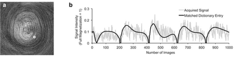
a: An example of the undersampled images from MRF-FISP. b: A representative time course of one pixel as indicated by the white circle in (a) and its matched dictionary entry. The estimated T₁ and T₂ values of this pixel are 750 ms and 65 ms, respectively. The longitudinal axis represents the fraction of the full magnetization that is equal to one.

T₁, T₂ and proton density maps generated from an asymptomatic volunteer are shown in Figure 8a, 8b and 8c. The acquisition was with an unbalanced gradient moment along the slice selection gradient. Supporting Figure S1 shows the results from the same volunteer with the sequence having an unbalanced gradient along the readout direction. The mean values of T₁ and T₂ of the region-of-interest in white matter and gray matter are within the range of previous literature results (28) as listed in Table 1. The noticeable difference between Figure 8 and Supporting Figure S1 are the estimated values from CSF, which is affected by the pulsation in CSF due to the change of unbalanced gradient direction. T₁-weighted images calculated from the maps in Figure 8 with TR = 250 ms and TE = 2.5 ms are shown in Figure 9a; T₂-weighted images in Figure 9b were calculated using TR = 10000 ms and TE = 90 ms; FLAIR (fluid-attenuated inversion recovery) images calculated with TI = 3600 ms, TE = 90 ms are shown in Figure 9c.

Figure 8.

T₁ (a), T₂ (b) and proton density maps (c) generated from an asymptomatic volunteer with the MRF-FISP acquisition. The unbalanced gradient moment along the slice selection gradient achieves 8pi dephasing per voxel.

Table 1.

T₁ and T₂ relaxation times and their standard deviations of MRF-FISP at 3 T, and the corresponding values reported in the literature (28).

			T2 (ms)	T2 (ms)
Tissue	MRF-FISP	Literature (28)	MRF-FISP	Literature (28)
White matter	781±61	788~898	65±6	78~80
Gray matter	1193±65	1286~1393	109±11	99~117

Figure 9.

a: T₁-weighted images calculated from the maps in Figure 8 with TR = 250 ms and TE = 2.5 ms; b: T₂-weighted images using TR = 10000 ms and TE = 90 ms and c: FLAIR images calculated with TI = 3600 ms, TE = 90 ms.

Discussion

Here we describe a FISP-based MRF method that can be used to quantify relaxation parameters. The results from phantom and in vivo human brain data suggest that accurate T₁ and T₂ values can be quantified by the proposed method.

Because of its unbalanced gradient within each repetition time, the simulation of the FISP sequence cannot be treated as a single isochromat in Bloch simulation for calculating the dictionary. While simulation of multiple spins is possible, it requires the simulation of hundreds or thousands of spins to achieve high accuracy, which could be time consuming. These results show that the extended phase graph formalism provides an alternative way to calculate the dictionary of MRF acquisition for sequences with the unbalanced gradient. Without the need to consider off-resonance, the dictionary size of FISP is also smaller compared to that of bSSFP at the same resolution of T₁ and T₂ values. This leads to an accelerated calculation time for the pattern-matching algorithm, or a potential increase in the dictionary resolutions of T₁ and T₂ values. While previous study (29) has illustrated that the variable repetition time causes a change in the signal amplitude of the FISP sequence with different off-resonance, our results show that T₁ and T₂ values can be quantified across a range of inhomogeneous B₀ using the MRF approach built upon pattern recognition. Off-resonance could have more effects on the quantitative results if the sequence employs a set of repetition times with stronger fluctuations, however, any effects such as off-resonance or slice-profile imperfections could be modeled and built into the dictionary used for pattern recognition to improve the final determination of the parameters.

The ability to simulate the gradient dephasing along with the RF pulse and the relaxation parameters gives us flexibility to include different type of sequences into MRF framework. This allows the sequence to employ longer repetition times, which could give more flexibility in sequence design, such as longer readout for higher spatial resolution or more variation in repetition times. It could also extend the MRF application to other organs or higher fields where it is potentially challenging for the bSSFP based sequence due to the banding artifact (30). It also has the potential to extend the method beyond MR relaxometry to quantify other physiological parameters, such as perfusion (31) and diffusion (32).

While the unbalanced gradient moment alleviate the banding artifact from bSSFP, FISP based MRF sequences could be affected by the increasing sensitivity to the motion along the unbalanced gradient direction (33). In brain applications, the most noticeable effect is in the cerebrospinal fluid that flows in and out the imaging slice with its long T₂ value. This results in the potential underestimation of the relaxation parameters in CSF in our proposed method.

Here we have only shown one of many examples in choices of flip angles and repetition times that are possible with a sequence such as MRF-FISP. We used the sinusoidal variation of flip angles and the pseudorandom repetition time to drive the magnetization into a persistent transient state that is sensitive to the relaxation parameters. The signal is driven to change smoothly so that the undersampling artifacts, physiological motion artifacts, and other artifacts from the systematic imperfection that varies in higher frequency can be ‘seen through’ in the pattern recognition algorithm. In the current study, the choice of the acquisition parameters was not fully optimized to generate the most efficient sequence. However, the proposed MRF-FISP method inherits the efficiency of the bSSFP-based MRF method and is able to achieve precisions of T₁ and T₂ values of less than 1% within 13 seconds of scan time. While we observed lower efficiency in MRF-FISP compared to MRF-bSSFP, the efficiency of both acquisitions are higher than the values reported in (13). This increase in efficiency can be attributed to the superior MRI hardware used in this study, including a higher main field magnet (3 T in current study, and 1.5 T in previous study (13)) and an improved multichannel array. We believe that a similar acquisition scheme can be used even in noncoherent steady state pulse sequence, such as FLASH, to quantify T₁, T *₂, or other parameters in the transient state. Optimizing the sequence parameters of MRF sequence will be an on-going effort because the degrees of freedom to design the sequence are nearly unlimited. The consideration of selecting a particular set of parameters for the MRF sequence needs to consider not only the sensitivity to the interesting parameters, but also image quality of parameter maps when the data are undersampled.

The “pseudo multiple replica method” is a robust measurement of noise when a direct measurement experiment is not possible. This approach represents a repeated measurements experiment, as long as the noise is Gaussian distributed. Non-Gaussian noises among the repetitions, such as noise from the instrument drift, physiological motion, and flow artifacts are not represented in this method.

Like all quantitative methods, the estimation of the parameters depends on how accurate the signal model reflects the actual acquired data. Several factors, such as imperfect slice profile, B₁⁺ inhomogeneity, and MT effect could affect the estimation of T₁ and T₂ (11,34). In this study, the dictionary was calculated with the ideal slice profile. The actual flip angle could be smaller than the nominal flip angle due to the imperfection of slice profile. In order to minimize the imperfect slice profile, a SINC RF waveform with the time bandwidth produce (TBP) of 8 was used. While the data are acquired using a RF pulse with a worse slice profile, slice profile correction (11) can be employed to mitigate the effect. A previous study (35) also showed the slice profile calculation can be included into EPG formalism to address this issue. An inhomogeneous transmit B₁ field would also affect the actual flip angle across FOV. While it is not severe in the phantom or brain application presented here, it could affect the results in the applications where larger FOV or more complicated coil setup is necessary. Either including B₁ into the dictionary, which is able to estimate B₁ simultaneously with the relaxation parameters (36) or adding an extra B₁ measurement, which matches the acquired signal to the corresponding dictionary with same B₁(30), would improve the quantification accuracy. The early study (30) has shown that B₁ effect in MRF sequence affects T₂ quantification more than T₁ quantification. Magnetization transfer (MT) effect is also known to affect T₁ quantification, especially in variable multiple flip angle methods (37,38). The transient state that MRF acquires is also sensitive to MT (39). The effect of MT is more apparent when using high power RF pulses with a short repetition time. Previous study (40) showed that reducing RF power by prolonging the RF pulse can be effective in reducing MT-related signal loss. MRF-FISP sequence is more flexible in terms of using longer repetition times and RF pulse duration because of the immunity to banding artifacts. In this study, we used RF pulses with 2 ms duration, and 11.5~14.5 ms repetition times, which has the potential to minimize MT effect in the sequence.

Though quantification of other physiological parameters, such as diffusion coefficients or perfusion, is out of scope of the current work, we believe the introduction of unbalanced gradient moment into MRF sequence opens new opportunities to quantify extra parameters besides T₁, T_2, and proton density.

References

- 1.Cheng H-LM, Stikov N, Ghugre NR, Wright GA. Practical medical applications of quantitative MR relaxometry. J. Magn. Reson. Imaging. 2012;36:805–24. doi: 10.1002/jmri.23718. [DOI] [PubMed] [Google Scholar]
- 2.Look DC. Time Saving in Measurement of NMR and EPR Relaxation Times. Rev. Sci. Instrum. 1970;41:250. [Google Scholar]
- 3.Deoni SCL, Rutt BK, Peters TM. Rapid combined T1 and T2 mapping using gradient recalled acquisition in the steady state. Magn. Reson. Med. 2003;49:515–26. doi: 10.1002/mrm.10407. [DOI] [PubMed] [Google Scholar]
- 4.Messroghli DR, Radjenovic A, Kozerke S, Higgins DM, Sivananthan MU, Ridgway JP. Modified Look-Locker inversion recovery (MOLLI) for high-resolution T1 mapping of the heart. Magn. Reson. Med. 2004;52:141–6. doi: 10.1002/mrm.20110. [DOI] [PubMed] [Google Scholar]
- 5.Zhu DC, Penn RD. Full-brain T1 mapping through inversion recovery fast spin echo imaging with time-efficient slice ordering. Magn. Reson. Med. 2005;54:725–31. doi: 10.1002/mrm.20602. [DOI] [PubMed] [Google Scholar]
- 6.Cheng H-LM, Wright GA. Rapid high-resolution T(1) mapping by variable flip angles: accurate and precise measurements in the presence of radiofrequency field inhomogeneity. Magn. Reson. Med. 2006;55:566–74. doi: 10.1002/mrm.20791. [DOI] [PubMed] [Google Scholar]
- 7.Heule R, Ganter C, Bieri O. Rapid estimation of cartilage T2 with reduced T1 sensitivity using double echo steady state imaging. Magn. Reson. Med. 2013 doi: 10.1002/mrm.24748. DOI: 101002/mrm.24748. [DOI] [PubMed] [Google Scholar]
- 8.Warntjes JBM, Dahlqvist O, Lundberg P. Novel method for rapid, simultaneous T1, T*2, and proton density quantification. Magn. Reson. Med. 2007;57:528–37. doi: 10.1002/mrm.21165. [DOI] [PubMed] [Google Scholar]
- 9.Warntjes JBM, Leinhard OD, West J, Lundberg P. Rapid magnetic resonance quantification on the brain: Optimization for clinical usage. Magn. Reson. Med. 2008;60:320–9. doi: 10.1002/mrm.21635. [DOI] [PubMed] [Google Scholar]
- 10.Schmitt P, Griswold MA, Jakob PM, Kotas M, Gulani V, Flentje M, Haase A. Inversion recovery TrueFISP: quantification of T(1), T(2), and spin density. Magn. Reson. Med. 2004;51:661–7. doi: 10.1002/mrm.20058. [DOI] [PubMed] [Google Scholar]
- 11.Ehses P, Seiberlich N, Ma D, Breuer FA, Jakob PM, Griswold MA, Gulani V. IR TrueFISP with a golden-ratio-based radial readout: fast quantification of T1, T2, and proton density. Magn. Reson. Med. 2013;69:71–81. doi: 10.1002/mrm.24225. [DOI] [PubMed] [Google Scholar]
- 12.Doneva M, Börnert P, Eggers H, Stehning C, Sénégas J, Mertins A. Compressed sensing reconstruction for magnetic resonance parameter mapping. Magn. Reson. Med. 2010;64:1114–20. doi: 10.1002/mrm.22483. [DOI] [PubMed] [Google Scholar]
- 13.Ma D, Gulani V, Seiberlich N, Liu K, Sunshine JL, Duerk JL, Griswold MA. Magnetic resonance fingerprinting. Nature. 2013;495:187–92. doi: 10.1038/nature11971. [DOI] [PMC free article] [PubMed] [Google Scholar]
- 14.Sekihara K. Steady-state magnetizations in rapid NMR imaging using small flip angles and short repetition intervals. IEEE Trans. Med. Imaging. 1987;6:157–64. doi: 10.1109/TMI.1987.4307816. [DOI] [PubMed] [Google Scholar]
- 15.Gyngell ML. The application of steady-state free precession in rapid 2DFT NMR imaging: FAST and CE-FAST sequences. Magn. Reson. Imaging. 1988;6:415–419. doi: 10.1016/0730-725x(88)90478-x. [DOI] [PubMed] [Google Scholar]
- 16.Hennig J, Weigel M, Scheffler K. Multiecho sequences with variable refocusing flip angles: Optimization of signal behavior using smooth transitions between pseudo steady states (TRAPS). Magn. Reson. Med. 2003;49:527–535. doi: 10.1002/mrm.10391. [DOI] [PubMed] [Google Scholar]
- 17.Deshpande VS, Chung Y-C, Zhang Q, Shea SM, Li D. Reduction of transient signal oscillations in true-FISP using a linear flip angle series magnetization preparation. Magn. Reson. Med. 2003;49:151–7. doi: 10.1002/mrm.10337. [DOI] [PubMed] [Google Scholar]
- 18.Wong ML, Wu EZ, Wong EC. Proceeding 22th Annu. Meet. ISMRM; Milan, Italy: 2014. Optimization of Flip angle and TR schedules for MR Fingerprinting. p. 1469. [Google Scholar]
- 19.Lee JH, Hargreaves BA, Hu BS, Nishimura DG. Fast 3D imaging using variable-density spiral trajectories with applications to limb perfusion. Magn. Reson. Med. 2003;50:1276–85. doi: 10.1002/mrm.10644. [DOI] [PubMed] [Google Scholar]
- 20.Hennig J. Multiecho imaging sequences with low refocusing flip angles. J. Magn. Reson. 1988;78:397–407. [Google Scholar]
- 21.Hennig J. Echoes—how to generate, recognize, use or avoid them in MR-imaging sequences. Part I: Fundamental and not so fundamental properties of spin echoes. Concepts Magn. Reson. 1991;3:125–143. [Google Scholar]
- 22.Weigel M. Extended phase graphs: Dephasing, RF pulses, and echoes - pure and simple. J. Magn. Reson. Imaging. 2014 doi: 10.1002/jmri.24619. [DOI] [PubMed] [Google Scholar]
- 23.Fessler JA, Sutton BP. Nonuniform fast fourier transforms using min-max interpolation. IEEE Trans. Signal Process. 2003;51:560–574. [Google Scholar]
- 24.Duyn JH, Yang Y, Frank JA, van der Veen JW. Simple correction method for k-space trajectory deviations in MRI. J. Magn. Reson. 1998;132:150–3. doi: 10.1006/jmre.1998.1396. [DOI] [PubMed] [Google Scholar]
- 25.Walsh DO, Gmitro AF, Marcellin MW. Adaptive reconstruction of phased array MR imagery. Magn. Reson. Med. 2000;43:682–90. doi: 10.1002/(sici)1522-2594(200005)43:5<682::aid-mrm10>3.0.co;2-g. [DOI] [PubMed] [Google Scholar]
- 26.Griswold MA, Walsh D, Heidemann RM, Haase A, Jakob P. The Use of an Adaptive Reconstruction for Array Coil Sensitivity Mapping and Intensity Normalization. Proc. Tenth Sci. Meet. Int. Soc. Magn. Reson. Med. 2002:2410. [Google Scholar]
- 27.Robson PM, Grant AK, Madhuranthakam AJ, Lattanzi R, Sodickson DK, McKenzie CA. Comprehensive quantification of signal-to-noise ratio and g-factor for image-based and k-space-based parallel imaging reconstructions. Magn. Reson. Med. 2008;60:895–907. doi: 10.1002/mrm.21728. [DOI] [PMC free article] [PubMed] [Google Scholar]
- 28.Wansapura JP, Holland SK, Dunn RS, Ball WS. NMR relaxation times in the human brain at 3.0 tesla. J. Magn. Reson. Imaging. 1999;9:531–8. doi: 10.1002/(sici)1522-2586(199904)9:4<531::aid-jmri4>3.0.co;2-l. [DOI] [PubMed] [Google Scholar]
- 29.Scheffler K. A pictorial description of steady-states in rapid magnetic resonance imaging. Concepts Magn. Reson. 1999;11:291–304. [Google Scholar]
- 30.Chen Y, Jiang Y, Ma D, Wright, Katherine L, Seiberlich N, Griswold MA, Gulani V. Proceeding 22th Annu. Meet. ISMRM; Milan, Italy: 2014. Magnetic Resonance Fingerprinting (MRF) for Rapid Quantitative Abdominal Imaging. p. 561. [Google Scholar]
- 31.Wright KL, Ma D, Jiang Y, Gulani V, Griswold MA, Hernandez-Garcia L. n Proceeding 22th Annu. Meet. ISMRM; Milan, Italy: 2014. Theoretical Framework for MR Fingerprinting with ASL: Simultaneous Quantification of CBF, Transit Time, and T1. p. 417. [Google Scholar]
- 32.Jiang Y, Ma D, Wright KL, Seiberlich N, Gulani V, Griswold MA. Proceeding 22th Annu. Meet. ISMRM; Milan, Italy: 2014. Simultaneous T1, T2, Diffusion and Proton Density Quantification with MR Fingerprinting. p. 28. [Google Scholar]
- 33.Santini F, Bieri O, Scheffler K. Proc. 16th Annu. Meet. ISMRM; Toronto, ON, Canada: 2008. Flow compensation in non-balanced SSFP. p. 3124. [Google Scholar]
- 34.Heule R, Bär P, Mirkes C, Scheffler K, Trattnig S, Bieri O. Triple-echo steady-state T2 relaxometry of the human brain at high to ultra-high fields. NMR Biomed. 2014;27:1037–45. doi: 10.1002/nbm.3152. [DOI] [PubMed] [Google Scholar]
- 35.Lebel RM, Wilman AH. Transverse relaxometry with stimulated echo compensation. Magn. Reson. Med. 2010;64:1005–14. doi: 10.1002/mrm.22487. [DOI] [PubMed] [Google Scholar]
- 36.Cloos MA, Wiggins C, Wiggins G, Sodickson DK. Proceeding 22th Annu. Meet. ISMRM; Milan, Italy: 2014. Plug and Play Parallel Transmission at 7 and 9.4 Tesla based on Principles from MR Fingerprinting. p. 542. [Google Scholar]
- 37.Ou X, Gochberg DF. MT effects and T1 quantification in single-slice spoiled gradient echo imaging. Magn. Reson. Med. 2008;59:835–45. doi: 10.1002/mrm.21550. [DOI] [PMC free article] [PubMed] [Google Scholar]
- 38.Mossahebi P, Yarnykh VL, Samsonov A. Analysis and correction of biases in cross-relaxation MRI due to biexponential longitudinal relaxation. Magn. Reson. Med. 2013 doi: 10.1002/mrm.24677. DOI: 10.1002/mrm.24677. [DOI] [PMC free article] [PubMed] [Google Scholar]
- 39.Gloor M, Scheffler K, Bieri O. Nonbalanced SSFP-based quantitative magnetization transfer imaging. Magn. Reson. Med. 2010;64:149–56. doi: 10.1002/mrm.22331. [DOI] [PubMed] [Google Scholar]
- 40.Bieri O, Scheffler K. Optimized balanced steady-state free precession magnetization transfer imaging. Magn. Reson. Med. 2007;58:511–8. doi: 10.1002/mrm.21326. [DOI] [PubMed] [Google Scholar]
Associated Data
This section collects any data citations, data availability statements, or supplementary materials included in this article.