Copula Regression Analysis of Simultaneously Recorded Frontal Eye Field and Inferotemporal Spiking Activity during Object-Based Working Memory

Abstract

Inferotemporal (IT) neurons are known to exhibit persistent, stimulus-selective activity during the delay period of object-based working memory tasks. Frontal eye field (FEF) neurons show robust, spatially selective delay period activity during memory-guided saccade tasks. We present a copula regression paradigm to examine neural interaction of these two types of signals between areas IT and FEF of the monkey during a working memory task. This paradigm is based on copula models that can account for both marginal distribution over spiking activity of individual neurons within each area and joint distribution over ensemble activity of neurons between areas. Considering the popular GLMs as marginal models, we developed a general and flexible likelihood framework that uses the copula to integrate separate GLMs into a joint regression analysis. Such joint analysis essentially leads to a multivariate analog of the marginal GLM theory and hence efficient model estimation. In addition, we show that Granger causality between spike trains can be readily assessed via the likelihood ratio statistic. The performance of this method is validated by extensive simulations, and compared favorably to the widely used GLMs. When applied to spiking activity of simultaneously recorded FEF and IT neurons during working memory task, we observed significant Granger causality influence from FEF to IT, but not in the opposite direction, suggesting the role of the FEF in the selection and retention of visual information during working memory. The copula model has the potential to provide unique neurophysiological insights about network properties of the brain.

Introduction

The frontal eye field (FEF), an area within the prefrontal cortex that is involved in visual spatial selection and attention control (Squire et al., 2013), has long been known to exhibit persistent delay period activity during memory-guided saccade tasks (Bruce and Goldberg, 1985). Recently, it has been shown that this persistent spatial signal may contribute to object-selective memory maintenance (Treisman and Zhang, 2006; Fougnie and Marois, 2009; Wood, 2011; Clark et al., 2012). In contrast, the inferotemporal cortex (IT), an end stage of the ventral “what” visual processing stream (Mishkin et al., 1983), is believed to be directly involved in object recognition (Logothetis and Sheinberg, 1996). IT neurons are known to exhibit persistent, stimulus-selective activity during the delay period of object-based working memory tasks (Chelazzi et al., 1993, 1998). Since neurons in FEF and IT, respectively, exhibit spatial-selective and object-selective delay activity, joint analysis of concurrent activity recorded in FEF and IT is crucial for understanding how the spatial signals in FEF interact with object information in IT during an object-based working memory task.

Standard approach for analyzing spike train interaction is performed either in the time domain or in the frequency domain (for review see Brown et al., 2004). Although these methods have played an important role in the analysis of spike trains, they are generally limited to a pair of neurons, lack of directionality of neural connectivity, and cannot be directly applied to the neural point process itself, i.e., sequences of spike times, but only to the smoothed versions of the spike trains or spike counts within some time bins, which would distort the properties of spike trains and introduce spurious effects. Other approaches include GLMs (Brillinger, 1988; Kass et al., 2014) and their variants where a spike train can be regarded as generated by a model in which the explanatory variables are either observed (the marginal GLM) or unobserved (the latent or state space). However, these methods present difficulties too. For example, the marginal GLM cannot model simultaneous occurrences of spike events, whereas the state-space model provides no principled way of choosing the number of latent dimensions. In addition, common methods for performing inference in state-space models with nonlinear and non-Gaussian observations rely on certain approximations that are not always accurate.

We develop a general and flexible likelihood framework that uses the copula to join marginal GLMs and handle the above challenges. To join marginal GLMs, a copula (Joe, 1997; Nelsen, 2006) is invoked as the link model, which naturally results in the copula GLMs. This paper demonstrates how the copula GLM attends to both sequential dependencies and shared influences on spiking activity. Additionally, this paper offers an approach akin to Granger causality measure for statistically identifying directional influence between spike trains. This method was tested on simulated data, compared favorably to the widely used GLMs, and finally applied to neural spike data collected simultaneously from the FEF and IT of a monkey while performing an object-based short-term memory task.

Materials and Methods

Experimental methods

General and surgical methods

Data were obtained from a male rhesus monkey (Macaca mulatta, 11 kg). The animal was surgically implanted with a titanium head post and a scleral eye coil. Surgery was conducted using aseptic techniques under general anesthesia (isoflurane), and analgesics were provided during postsurgical recovery. Structural magnetic resonance imaging was performed to locate the arcuate sulcus in the monkey for the placement of a recording chamber in a subsequent surgery. A craniotomy was performed on the animal, allowing access to the FEF on the anterior bank of the arcuate sulcus. All experimental procedures were in accordance with the National Institutes of Health Guide for the Care and Use of Laboratory Animals, the Society for Neuroscience Guidelines and Policies, and Stanford University Animal Care and Use Committee. General surgical procedures have been described previously (Armstrong et al., 2006).

Visual stimuli and behavior

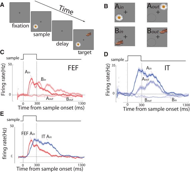
Throughout the experimental session, the monkey was seated in a primate chair and eye position was monitored with a scleral search coil with a spatial resolution of <0.1° (Armstrong et al., 2006) and was digitized at 100–200 Hz. The monkey was trained to fixate within a 1.5–3° diameter error window surrounding a central spot (0.4° diameter). Delayed match-to-sample (DMS) task is depicted in Figure 8A. At 250–750 ms after fixation, a colored photo image (5° diameter) was presented for 300 ms (sample period). A delay period of 1000 ms followed the sample offset (delay period), after which two potential target images appeared on screen (target period), and the monkey had to saccade directly to the repeated image to obtain a juice reward. The monkey was required to maintain fixation throughout the sample presentation and delay; breaks in fixation before the trial was completed were considered aborted trials and were not included in the data analysis. Three images were used in each experimental session, and all three images appeared with equal frequency as samples and nonmatching distractors in the target array. The location of the matching target was randomized with respect to sample location. Target array configuration (aligned with sample locations vs orthogonal to sample locations) was held constant for 250–400 trials, then switched for the remainder of an experimental session; initial target array position for each session was selected at random. All sample location, sample identity, and nonmatch target identity conditions were pseudorandomly interleaved and were controlled by the Cortex system for data acquisition and behavioral control. During each experiment, the two sample positions were selected so that one stimulus was positioned inside the response field (RF) of the FEF neuron being recorded, based on the endpoints of saccades evoked with microstimulation (7–13° visual angle). The monkey was initially trained exclusively on the orthogonal-targets version of the task, and only learned the aligned-targets version after reaching criterion (70%) performance with the orthogonal targets. All visual stimuli were displayed on a liquid crystal display monitor (52 cm vertical × 87 cm horizontal) positioned 57 cm in front of the monkey, with a refresh rate of 60 Hz. Stimulus presentation was controlled and recorded by Cortex.

Figure 8.

Experimental task and the activity of FEF and IT neurons during the object-based delayed match-to-sample task. A, Schematic of the object-based DMS task: the monkey fixates at the small central spot. A sample image appears on either inside of or opposite the FEF RF for 300 ms (sample period). The monkey maintains fixation throughout 1 s (delay period), during which only the fixation spot remained on the screen. The match and nonmatch images appear at positions inside and opposite the RF, and the monkey saccades to the match to receive a reward (target period). The location of the match is randomized with respect to the sample image position. B, The locations of the sample images presented inside (A_in and B_in, left column) or outside (A_out and B_out, right column) the FEF RF. The dashed-line circles indicate hypothetical RFs for FEF site. C, The response of FEF neurons is spatially selective when sample appeared inside the FEF RF (A_in and B_in) versus outside the FEF RF (A_out and B_out), regardless of the sample type. D, The response of IT neurons is object selective for one type of sample (A_in and A_out) versus another type of sample (B_in and B_out), regardless of its location. E, The response of FEF neurons occurs earlier than that of IT neurons when sample object appeared inside the FEF RF and was preferred for the IT neurons.

FEF and IT neuronal recordings

Single-neuron recordings in awake monkey were made through a surgically implanted cylindrical titanium chamber (20 mm diameter) overlaying the arcuate sulcus. Electrodes were lowered into the cortex using a hydraulic microdrive (Narishige). Activity was recorded extracellularly with varnish-coated tungsten microelectrodes (FHC) of 0.2–1.0 MΩ impedance (measured at 1 kHz). Extracellular waveforms were digitized and classified as single neurons off-line using both template-matching and window-discrimination techniques (FHC, Plexon).

During each experiment, a recording site in the FEF was first localized by the ability to evoke fixed-vector, saccadic eye movements with stimulation at currents of <50 μA (Bruce et al., 1985). Electrical microstimulation consisted of a 100 ms train of biphasic current pulses (0.25 ms, 200 Hz) delivered with a Grass stimulator (S88) and two Grass stimulation isolation units (PSIU-6; Grass Instruments). Current amplitude was measured via the voltage drop across a 1 kΩ resistor in series with the return lead of the current source. During each experimental session, we mapped the saccade vector elicited via microstimulation at the cortical site under study with a separate behavioral paradigm (Moore and Fallah, 2001). In this paradigm, the monkey was required to fixate on a visual stimulus (0.48° diameter circle) for 500 ms, after which time a 100 ms stimulation train was delivered on half the trials. Evoked saccades had vectors with lengths ranging from 4 to 15° visual angle and angles of −60 to 270° theta. After mapping the saccade vector, we recorded the response of any neuron that could be isolated by advancing the electrode within 0–250 μm of the stimulation site (average distance from stimulation site was <100 μm) while monkeys performed the DMS task.

Single-neuron recordings in IT were made through the same surgically implanted cylindrical titanium chamber (20 mm diameter) used for FEF recordings. Targeting of IF area TE was based on structural MRI data acquired before well placement, the pattern of gray and white matter encountered when advancing the electrode, and the response properties of neural recordings. A 32 gauge (235 mm outer diameter) guide tube was advanced ∼15 mm through the brain (at a rate of ∼0.75 mm/min) by a custom-modified, electronic motor-driven microdrive, stopping at or just above the upper bank of the superior temporal sulcus. An electrode (75–100 μm diameter) was then advanced another 5–12 mm using a hydraulic microdrive (Narishige). Neural spikes were obtained via off-line sorting (FHC, Plexon), and saved at the sampling rate of 1 kHz.

After isolating a unit within IT, the cell was screened for selective visual responses using Rapid Serial Visual Presentation (RSVP) of a bank of 40 color object images. During the RSVP paradigm the monkey fixated while a series of object images appeared at the fovea behind the fixation point. Each image was displayed for 150 ms, followed by a 100 ms gap before the next image appeared; 10 images appeared in series on each trial, with the order of their appearance randomized from trial to trial. Spikes were collected and counted on-line in Cortex for a 150 ms bin beginning 100 ms after image onset. After a minimum of five presentations of each image, responses were evaluated for selective visual response to one or more of the objects; if no selectivity was apparent after ∼20 trials of each type, the electrode was advanced in search of a new isolation. For selective units, at least one good and one poor stimulus was chosen to serve as stimuli in the DMS task for that day. Depending on isolation quality, the preparation was often allowed to “settle” for 15–30 min following this RSVP assessment of visual selectivity. For this reason, and because separate units were sometimes identified from a single recording with subsequent off-line spike sorting, and because the strength of visual responses sometimes changed when the stimuli were moved to the periphery for the DMS task, selectivity of IT units was reassessed using responses during the DMS task itself. Only cells with significant visual response and selectivity during the DMS task (assigning preference based on a subset of trials excluded from further analysis and assessing significance in the remaining trials) were included in analysis.

Statistical methods

In this section, we introduce the statistical theory underlying our approach. First, we provide a brief review of the copula theory. Second, we present the copula-based joint GLM for multiple spike train data analysis. Third, we derive a simultaneous, maximum likelihood estimation procedure that is implemented by a Gauss–Newton type algorithm. Finally, we describe a Granger causality measure based on the likelihood ratio statistic for the analysis of neural spike trains. The C and MATLAB codes implementing this algorithm can be provided to interested readers upon request.

Copula

Extensive treatment of copula models can be found in the literature (Joe, 1997; Nelsen, 2006). Here we summarize the main elements needed for this work.

In probability theory, a copula is a function that links (couples) the univariate marginal distributions to a multivariate joint distribution. With copula, one can dissociate the marginal distributions from their joint density distribution and, therefore, focus on only statistical dependence between variables. Sklar's Theorem (Sklar, 1973) is central to statistical theory of copula, stating that any multivariate distribution can be expressed as the copula function evaluated at each of the marginal distributions. Formally, let X = (x₁, …, x_N) be a vector random variable with corresponding cumulative probability distribution (CDF) F defined on R^N. The copula associated with F is a distribution function C: [0, 1]^N → [0, 1] that satisfies F(X) = C(F₁(x₁), …, F_N(x_N)), X ∈ R^N. If F is a continuous distribution on R^N with univariate marginals F₁, …, F_N, then C(u) = F(F₁⁻¹(u₁), …, F_N⁻¹(u_N)) is unique. Assuming that F has Nth order partial derivatives, its probability density function (PDF) can be obtained from the distribution function via differentiation: f(X) = $\frac{{\partial }^{N}F\left(X\right)}{\partial x_1\dots \partial x_N}$. The PDF can be rewritten in terms of derivatives of copulas: f(X) = $\frac{{\partial }^{N}F\left(X\right)}{\partial x_1\dots \partial x_N}=\frac{{\partial }^{N}C\left(u\right)}{\partial u_1\dots \partial u_N}{\displaystyle {\prod }_{i=1}^N\frac{\partial u_i}{\partial x_i}=c\left(u\right){\displaystyle {\prod }_{i=1}^N{f}_i\left(x_i\right)}}$, where c(u) = $\frac{{\partial }^{N}C\left(u\right)}{\partial u_1\dots \partial u_N}$ is referred to as copula density function, and f_i(x_i) refers to the individual marginal probability density function.

The main advantage of copulas is that they allow us to model the marginal distributions separately from the multivariate dependence structure (copula) that links them together into the multivariate model of study. Copulas are thus building blocks for multivariate distributions. It is common practice to assume a parametric model for the estimation of the copula functions that allow for different dependence structures and often have quite simple functional forms. As such, we use the Gaussian copula in this work due to its scalability and its flexible dependence structure (Nelsen, 2006). Note that independent copula is the simplest example with constant density of 1, i.e., c(u) = 1.

Copula-based joint GLM for neural spike trains

Model description.

Our approach is built upon the popular marginal GLM and the copula theory to model multivariate point process of spike trains. The marginal GLM (Brillinger, 1988; Chornoboy et al., 1988; Brown et al., 2003; Okatan et al., 2005; Truccolo et al., 2005; Pillow et al., 2008; Stevenson et al., 2008) only assumes that the neuron's spike is influenced by such factors as its own spiking history and the concurrent ensemble history of other neurons, without considering their joint response dependency (i.e., simultaneous occurrences of spikes from multiple neurons). In contrast, the copula-based method that we previously developed (Li et al., 2006; Song et al., 2009; He et al., 2012) only considers the joint dependency of the variables as specified by some copula, without modeling the time-lagged history information of dependent variables. As such, our model is an extension of our previous work by incorporating the temporal dependence information between the variables into the copula models. The proposed approach, to our knowledge for the first time, represents the time-lagged information in the copula models.

To formulate the point process representation of spike trains, we start with conditional intensity function (CIF) of point process (Daley and Vere-Jones, 2003), which is the key to approximating the neuron's spiking probability in the well-developed GLM framework. Let 0 < t₁^m < … < t_Jm^m ≤ T be a set of J_m spike times observed in the time interval (0, T) for m = 1, …, M recorded neurons, and let N_j(t) denote the number of spikes for neuron j in the time interval (0, t) for t ∈ (0,T). A point process model of a spike train for a neuron j can be completely characterized by its conditional intensity function, λ_j(t|H_j(t)), which is defined as follows: λ_j(t|H_j(t)) = $\begin{array}{c}\lim \\ \Delta \to 0\end{array}\frac{P\left[N_j\left(t+\Delta \right)-N_j\left(t\right)=1|H_j\left(t\right)\right]}{\Delta }$, where P[.|.] is a conditional probability, and H_j(t) refers to the ensemble spiking history up to time t. The probability that neuron j fires a single spike at a small interval from t to t + Δ can be approximated as λ_j(t|H_j(t))Δ, which is affected by such covariates as its own spiking history, the concurrent ensemble history of other neurons, and the activity of some external variables. The CIF of a neuron j, λ_j(t|H_j(t)), as defined above, is modeled via GLM by including all covariates of interest:

where g is an appropriate link function, which is the logit for the Bernoulli model or the log for the Poisson model; both are equivalent for small enough Δ when applied to neural spike trains (Truccolo et al., 2005). The first term β_j,0 denotes the baseline firing activity of neuron j. The second term captures the effect of ensemble spiking history on neuron j, with the coefficient β_j,k,l indicating the magnitude of effect of spiking history H_k,l(t) for neuron k at the time lag l. The last term models the effect of some external variables, with β_j,s denoting the dependency of neuron j on the external covariates Z_s. Let Q_j(t) denote the information set for neuron j up to time t, consisting of all ensemble spiking history H_k,l(t) and extrinsic covariates Z_s(t), Q_j(t) = {H_1,1, H_1,2, …, H_K,L, Z₁, Z₂, …, Z_S}. The parameter vector β_j for neuron j is given as follows: β_j = {β_j,0, β_j,1,1, β_j,1,2, … β_j,K,L, β_j,1, β_j,2, …, β_j,S}.

To ease the construction of the model estimation, a discrete time representation of the point process can be obtained via partitioning the observation interval (0, T) into k = 1, …, K subintervals (t_k−1, t_k), each of length Δ = TK⁻¹ such that at most one spike per subinterval is observed. Typically, K is chosen to make Δ as 1 ms due to the refractory period of neurons. In discrete time representation, we use N_j[k] for N_j(t_k), Q_j[k] for Q_j(t_k), and the parametric form of the conditional intensity function becomes λ_j(t_k|β_j, Q_j[k]). Having obtained explicit the parametric model of the conditional intensity function for each neuron, next we show how to use the copula to integrate marginal regression models of spike trains into a joint analysis.

To analyze neural spike trains within a given time period, assume X_j, j = 1, …, M to be M binary random variables with the probability of spike firing p_j. The CDF of X_j can be written as below:

Consider a simple case of two spike trains, X₁ and X₂, with M = 2, the bivariate joint probability mass function follows the two-increasing property (Nelsen, 2006):

where u_j = F_j(x_j) and v_j = F_j(x_j − 1). Here C can be the bivariate Gaussian copula: C(u, v|r) = Φ₂(Φ⁻¹(u), Φ⁻¹(v)|r), where Φ₂ is the CDF of a bivariate Gaussian with marginal variances equal to one and correlation r, and Φ⁻¹ is the normal score or quantile function of the standard Gaussian distribution. The joint distribution function between X₁ and X₂ has four elements:

To obtain the spiking probability of a neuron, p_j, in the above equation, we consider the generalized linear point-process model described in Equation 1 as the marginal distributions, where the logit, or the inverse of logistic function, is used as the link function, resulting in the well known logistic regression model. The conditional intensity function λ_j(t_k|β_j, Q_j[k]) of Equation 1 represents the firing rate of neuron j at time t in the kth bin/subinterval given its covariates Q_j[k], which can then be used to approximate the spiking probability of a neuron, p_j, in Equation 3. When a copula instead of Gaussian copula is used, the joint probability is different. Therefore, based on the joint distribution in Equation 3, we can perform maximum likelihood inference to estimate all the model parameters. This leads to our bivariate copula GLM model.

To generalize the joint probability mass function for two neurons in Equation 2 to multiple neurons, we obtain a multivariate joint probability mass function as follows (Song, 2007):

where u_j,1 = F_j(x_j) and u_j,2 = F_j(x_j − ). Here F_j(x_j − ) is the left-hand limit of F_j at x_j, which is equal to F_j(x_j − 1) when the support of F_j takes integer values as for the Bernoulli or Poisson distributions.

The joint probability of our model depends on the copula correlation parameter r and the regression parameters β (β_j, j = 1, …, M, where M is the number of neurons). For Gaussian copula, a consistent and asymptotically normally distributed estimator of the parameters can be obtained through maximum likelihood. Assuming multiple spike trains of certain observations, the overall likelihood is simply the product of the likelihoods across all the observations. Akaike information criterion (AIC; Akaike, 1974) can be used to determine the model order.

Parameter estimation by maximum likelihood.

In this section, our primary task is to establish a simultaneous maximum likelihood estimation for the model parameters θ = (β, r). Let ℓ(θ) denote the log-likelihood function of the model. Then the maximum likelihood estimation of θ is obtained by θ̂ = arg max (ℓ(θ)). In this case, the popular Newton–Raphson or the Fisher scoring algorithms are not suitable, because in most of situations the second-order derivatives of the log-likelihood are not available. As such, we instead make use of the Gauss–Newton type algorithm (Ruppert, 2005; Li et al., 2006; Song et al., 2009; He et al., 2012), which only requires the first derivatives of the log-likelihood function. The parameters are updated by step-halving to ensure that the likelihood increases progressively over iterations. Specifically, the (k + 1)th iteration updates the parameters θ by the following:

where B_n = $\frac{1}{n}{\displaystyle {\sum }_{i=1}^n\left(\frac{\partial \ell (\theta )}{\partial \theta }\right){\left(\frac{\partial \ell (\theta )}{\partial \theta }\right)}^T}$ and ε is the step-halving term that starts from 1 and halves until ℓ(θ^k+1) > ℓ(θ^k) at iteration k. The algorithm stops when the increase in the likelihood is no longer possible or the difference between two consecutive updates is smaller than a predefined precision level. We initialize the parameters β with Gaussian random numbers and the correlation parameter r with the Pearson correlation between spike trains. We use the unconstrained nonlinear optimization algorithm (the MATLAB function fminunc) to search for the values of β that minimize the negative log-likelihood of the full set of observed spikes. The fminunc can supply numerical Hessian matrix, which can be used to evaluate the variances of the estimated parameters. Following the model fitting, we assess the goodness-of-fit (GOF) of the estimated model with the Kolmogorov–Smirnov (KS) plots (Brown et al., 2002).

Granger causality measure for point process.

Identifying the causal relationship between spike trains is an important, yet challenging, problem in computational neuroscience. Granger causality has proven to be an effective method for the analysis of the directional interactions between continuous-valued time series in many applications (for review, see Kaminski and Liang, 2005 and the references therein). It is, however, not directly applicable to spike train data due to their discrete nature. Although a few attempts have been made to tackle the problems (Nedungadi et al., 2009; Krumin and Shoham, 2010), they all require the spike train data to be second-order stationary. Recently, a point process method incorporating the full conditional intensity function for measuring Granger causality between neurons was proposed (Kim et al., 2011). This method is based on the marginal GLM where Granger causality is assessed via the likelihood ratio statistic, which measures the extent to which the likelihood of one neuron is reduced by excluding one of its covariates compared with the likelihood obtained using all of its covariates. As our copula-based joint GLM method is a multivariate extension of the marginal GLM, it is straightforward to adopt a similar strategy to assess Granger causality for spike trains data while retaining all the desired properties of the marginal GLM, but with better model estimation, as demonstrated by both simulations and actual neural data in Results.

To introduce the key idea, assume we have two spike trains X and Y. We first establish a full model for these spike trains with the copula-based joint GLM, in which the spiking histories of neurons X and Y as the covariates are considered. For instance, the marginal GLMs of X and Y of model order P, with logit link function in Equation 1, can be specified as follows:

where β refers to the unknown parameter vector, and λ refers to the probability of spike firing represented by the CIF. The marginal GLMs of X and Y are joined by a copula model of a copula parameter r, with the joint distribution function given in Equation 4. The model parameters θ = (β, r) can then be estimated by our maximum likelihood procedure as described above, and the likelihood of the full model can be obtained as L_full.

The reduced model representing potential causal influence from neuron Y to neuron X is then separately established by excluding the spiking history of neuron Y in the regression function of X, i.e.,

Following the same estimation procedure as the full model, we obtain the likelihood of the reduced model (L_reduced^Y→X). Granger causality of Y→X can thus be assessed by the log-likelihood ratio of the full model and reduced model:

Granger causality of X→Y can be calculated in a similar way. Since the likelihood of the full model is always greater than or equal to the likelihood of the reduced model, the log-likelihood ratio (and hence Granger causality) is greater than or equal to zero. Granger causality measure given by Equation 5 provides an indication of the extent to which the neuron Y affects the neuron X by considering both the influence of the spike history and the influence of the simultaneous spike occurrences. This procedure leads to the bivariate Granger causality for point processes.

For multivariate point-process time series, bivariate Granger causality is often insufficient to distinguish the direct causality from indirect causality, thus resulting in the misleading inference. Conditional Granger causality can be used to address this issue (Ding et al., 2006). Our approach is readily extended to multivariate time series simply by including the time-lagged history information of other variables into the regression. The statistical significance of the estimated Granger causality can be assessed parametrically with an asymptotic χ² distribution described previously (Kim et al., 2011). We instead use the nonparametric permutation procedure, in which a Granger causality distribution expected by chance can be obtained via independently shuffling trial order for each pair of spike trains.

Results

Copula regression analysis of simulated spike train data

We designed a series of simulations to investigate the performance of our copula GLM for the analysis of spike train data. The first simulation is to evaluate the performance gain of our copula-based joint GLM analysis in improving estimation accuracy and the robustness of our model to simultaneous occurrences of spike events as compared with the marginal GLM. The second simulation is to assess the ability of our copula model in detecting synchrony in the presence of simultaneous occurrence of spike events and compare it with recent methods (Kass et al., 2011; Kelly and Kass, 2012) in addition to the marginal GLM. The third and fourth simulations, respectively, examine the effect of the trial number and spiking rate on the performance of our algorithm. The final simulation illustrates the utility of the Granger causality measure in the analysis of spike train data. To avoid confusion in terminology, we denote our proposed copula-based joint GLM method as the copula GLM, and the popular point-process GLM method as the marginal GLM.

Methodology assessment

We simulated a simple recursive model for a pair of binary-dependent variables (X₁, X₂), in which the probabilities of events (p₁, p₂) are described by logit margins: $\{\begin{array}{cc}{X}_1:& \log it\left(p_1\right)={\beta }_1+{\beta }_2{X}_{1,t-1}+{\beta }_3{X}_{2,t-1}+{\beta }_4{Z}_1+{\beta }_9{X}_{2,t}\\ X_2:& \log it\left(p_2\right)={\beta }_5+{\beta }_6{X}_{1,t-1}+{\beta }_7{X}_{2,t-1}+{\beta }_8{Z}_2\end{array}$, where Z₁ and Z₂ follow a normal distribution N(0, 1), representing the extrinsic covariates such as stimuli or behavior. The contemporaneous dependence due to shared inputs and network interactions for (X₁, X₂) is modeled via the Gaussian copula with a correlation parameter r. We set β₁ = −1, β₂ = −0.5, β₃ = −0.3, β₄ = 0.4, β₅ = −1, β₆ = −1, β₇ = −0.2, β₈ = 0.6, and β₉ = 0, unless otherwise specified. This model is designed to include not only the time-lagged effect, which is reflected by the model coefficients (β₂, β₃, β₆, β₇,), but also the synchronous spiking, i.e., simultaneous occurrences of spike events, which is reflected by the model coefficients (β₉), in addition to the extrinsic covariate effects (β₄, β₈) due to network activity such as the slow-wave activity (Kelly et al., 2010; Kelly and Kass, 2012).

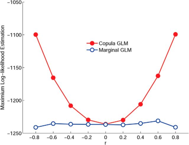
We systematically vary the correlation parameter r from −1 to 1 with the increment of 0.2. For each r, we generate a dataset consisting of 200 trials of randomly synthesized pairs with 1000 sample points. Accordingly, we apply the copula GLM and the marginal GLM models to fit each dataset, respectively. We compared the performances of the two models in terms of the resultant maximum likelihoods and estimated parameters. Figure 1 shows the averages of maximum log-likelihoods of the data with different correlation parameters obtained through the copula GLM (red) and the marginal GLM (blue) models. As expected, the log-likelihood profile exhibits symmetry for positive and negative correlation. Importantly, as reflected in the maximum log-likelihoods, our method is able to capture the different dependence structures of varying correlations between point processes, whereas the marginal GLM only provides comparable log-likelihoods across different datasets, unable to distinguish the different dependence structures contained in the data.

Figure 1.

Maximum log-likelihood estimation by the marginal GLM (blue) and the proposed copula GLM (red) for various simulated datasets that were generated with the same marginal parameters β but different correlation parameter r. Clearly, compared with the marginal GLM, the copula GLM is able to capture the different dependence structures in the data.

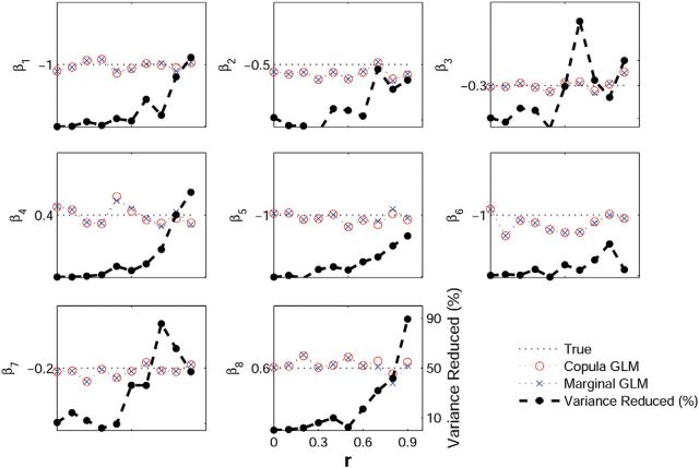
To compare the accuracy of parameter estimation between two models, we show the results in Figure 2 where only positive correlation is presented due to the symmetry in correlation and for the sake of clarity. Based on the average of estimated parameters obtained by the copula GLM and the marginal GLM (Fig. 2, left, y-axis, circles and crosses, respectively), we can see that both methods show general agreement on the parameter estimation. However, as the correlation increases, we find that the copula GLM model in general produces smaller variance in the estimated parameters than the marginal GLM, as shown by the percentage reduction of the variance estimated by the copula GLM relative to the marginal GLM (Fig. 2, right, y-axis). In addition, the marginal GLM model is not able to estimate the correlation parameter r, yet the copula GLM provides accurate estimation. These results indicate that the marginal GLM can only describe the lagged dependence. With the presence of the instantaneous dependence between spike trains the parameters estimated by the marginal GLM become inaccurate, resulting in larger variance. We note that both common inputs and additive noise may give rise to instantaneous dependence that can strongly affect model estimation, but they are fundamentally different: the effect of common inputs via shared sources can be accounted for by explicit modeling (Ba et al., 2014) or by some unobserved hidden states in the state-space GLM (Paninski et al., 2010), whereas additive noise is much difficult to model as it only affects current, but not future, observations. Our copula GLM can account for both effect of common inputs and additive noise, with the additive noise explained by the copula parameter.

Figure 2.

Parameter estimation via the copula GLM (red circles) compared with the marginal GLM (blue crosses) for datasets with the different correlation parameters r. In each part, the left y-axis corresponds to the average of a given parameter estimated over 200 trials by the two methods as a function of the correlation parameter, with its true value labeled on the y-axis (dotted horizontal lines), whereas the right y-axis denotes the percentage of the estimation variance reduced by using the copula GLM as compared with the marginal GLM (black dashed curves with filled circles). We see the general agreement on the average parameter estimated by the two methods, but the copula GLM provides a more accurate estimation of smaller variance than the marginal GLM, particularly for the datasets with increased correlation parameters.

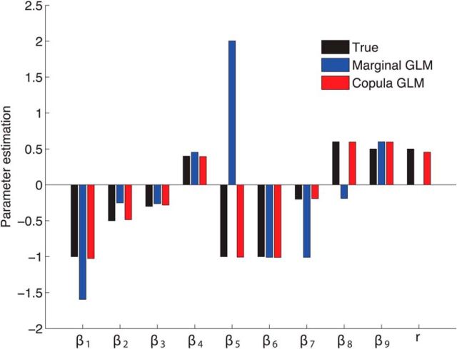
To further validate the above results, we explicitly induce the zero-lag, instantaneous influence into the model by setting β₉ = 0.5 while keeping all other parameters unchanged. Note that an instantaneous covariate X₂ is now included in the regression of X₁ to produce the zero-lag effect. We generate the simulated spike train data based on the model with the copula correlation parameter r = 0.5. We then repeat the same analysis procedure as above, with Figure 3 showing the results of parameter estimation. It is evident from Figure 3 that our copula GLM method still recovers all the model parameters very well, whereas the marginal GLM fails to provide the correct model estimation.

Figure 3.

Comparison of the average parameters estimated by the copula GLM (red) and the marginal GLM (blue) for the analysis of the simulated spike train data. It is clear that the copula GLM provides more accurate parameter estimation than the marginal GLM, as compared with the true values (black). Note that the copula GLM, but not the marginal GLM, is able to estimate the correlation parameter.

Performance comparison for detecting synchrony

Simultaneous occurrence of spikes from multiple neurons is a hallmark of neuronal synchrony. In practice, it is not always known in advance whether there is an instantaneous effect in a given dataset. Therefore, it is important to assess to what extent our copula GLM can still account for such instantaneous influence without explicitly modeling the zero-lag effect, and how our model is compared with the other approaches such as Kass et al. (2011) and Kelly and Kass (2012). As such, we use the same model above to generate spikes with different instantaneous influence by varying copula correlation parameter r from 0 to 1 with a step size of 0.1. In general, we observe a monotonically increasing relationship between the values of copula correlation parameter r and the increase in synchrony rate relative to r = 0. For example, when r = 0.1, 0.5, and 0.9, the relative increased rates are, respectively, 17, 83, and 180%. We note that the copula correlation parameter is different from the commonly used correlation that should be interpreted with caution, particularly for measuring synchrony (Brody, 1999a, b). First, it detects only linear relationship, whereas dependence in copulas is nonlinear in general. Second, and relatedly, it is not invariant to transformation of the marginal distributions.

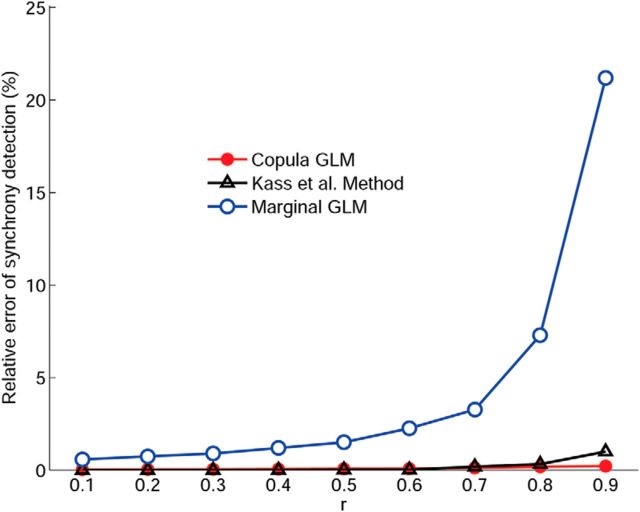
To facilitate the comparison between different models, we quantify the performance of synchrony detection as the relative error, which is the difference between the detected and the true probability of synchronous events relative to the true probability of synchronous events. For the simulated data, we perform both the copula GLM and the marginal GLM without the instantaneous term X₂ included as the predictor in the regression of X₁ and compare with the Kass method (Kass et al., 2011; Kelly and Kass, 2012). Figure 4 shows the comparison of the relative errors among three methods. We can see that, even when the simultaneous term X₂ is not explicitly modeled, our copula GLM still provides better synchrony detection, in fact very close to the actual spiking events, than the marginal GLM. As expected, the marginal GLM does not perform well, particularly when the copula correlation parameter is high. Interestingly, both the copula GLM and Kass method show comparable performance, although the former gives slight edge over the latter when the copula parameter becomes large. The robustness of our method can be attributed to the use of copula to model the joint dependency to account for simultaneous occurrences of spike events. Therefore, although the zero-lag, instantaneous influence is not explicitly modeled in the regression process, such information is still captured by the copula parameter. This is a major advantage over the marginal GLM.

Figure 4.

Comparison of the relative errors of synchrony detection among the copula GLM (red), marginal GLM (blue), and the Kass method (black). The results show that the marginal GLM performs poorly when the simultaneous term is not explicitly modeled, yet the copula GLM still maintains very low relative error, even when the copula correlation parameter becomes large. In addition, our copula GLM has comparable performance with the Kass et al. (2011).

Effect of trial number on model performance

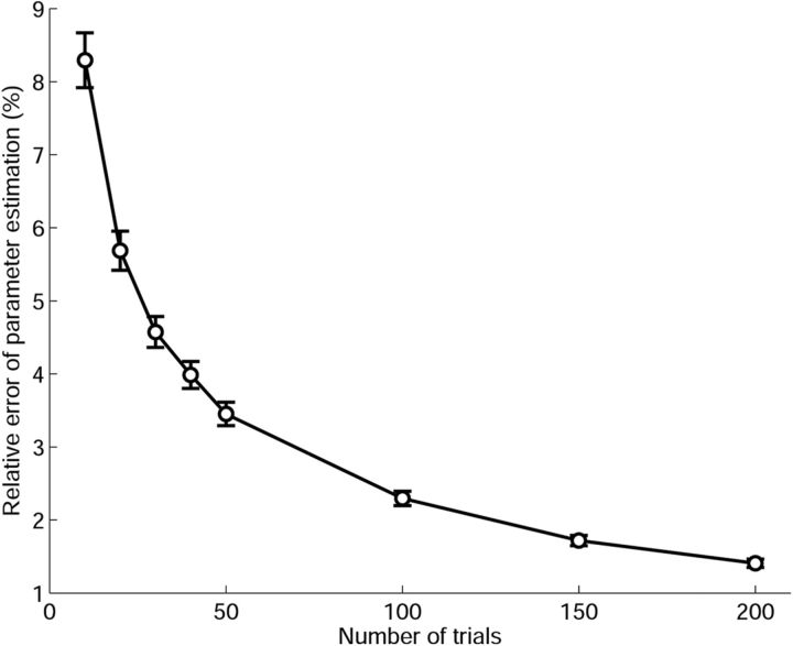
In this simulation, we evaluate the performance of our model in terms of different numbers of trials (10, 20, 30, 40, 50, 100, 150, and 200). We generate the data according to the model in the first simulation with the spiking rates close to real neural data below. The model performance is computed as the relative error of the estimated parameters, which measures the deviation of estimated value from true value of model parameter relative to the true model parameter. For a given trial number, we repeat the same model-fitting procedure for many times (1000 in the simulation) to obtain the error bar. Figure 5 shows the result, where we can see that all relative errors of parameter estimation are <10%, and when the trial number is >30, the relative error is controlled within 5%.

Figure 5.

The effect of trial number on the model performance. We can see that the relative error of parameter estimation decreases as the number of trials increases. With as few as 30 trials, the relative error can be controlled within 5%. Error bars denote SEM.

Effect of spiking rate on model performance

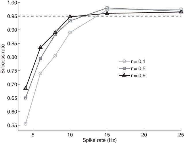
We conduct the performance analysis of our algorithm to different neural firing rates and copula correlation parameters. We choose a simple bivariate point process (X₁, X₂) with the logit marginal descriptions: (X₁, X₂), with the logit marginal descriptions: $\{\begin{array}{cc}{X}_1:& \log it\left(p_1\right)={\beta }_1+{\beta }_2{Z}_1\\ X_2:& \log it\left(p_2\right)={\beta }_3+{\beta }_4{Z}_2\end{array}$. Here, Z₁ and Z₂ follow a normal distribution N(0, 1). The joint dependency of (X₁, X₂) is modeled via a Gaussian copula with the correlation parameter r. For each given parameter r (0.1, 0.5, and 0.9), we generate datasets with the different firing rates ranging from 4 to 25 Hz (i.e., 4, 6, 8, 10, 15, and 25 Hz) by changing the model parameters β. For each combination of r and the firing rate β, we have a dataset consisting of 400 trials, each of 1000 sample points, on which the copula GLM is applied. We estimate the model parameters θ = (β, γ) for each trial. We use the Fisher information I(θ) to construct the approximate confidence intervals of estimated parameters. It has been shown that the bias of an estimated parameter away from its true value follows a normal distribution: $\sqrt{n}$(θ − θ̂) ∼ N (0, I⁻¹(θ)) under regularity conditions, where n is the number of sampling points (Serfling, 1980). If any of the estimated parameters is out of the confidence interval at a certain significant level α (e.g., 0.05), this estimation is rendered unsuccessful. We conduct the performance analysis of our copula framework by examining the rate of success at various parameter settings. Figure 6 shows the results of performance analysis, where the success rates of our copula GLM model change as a function of spiking rate at different correlation parameters, r. We observed from Figure 6 that (1) the larger r facilitates the estimation of model parameters, especially in the low firing rate region (< 15 Hz) and (2) the spike firing rate of ∼15 Hz is required for the model to achieve the parameter estimation at the 95% success rate (the horizontal dashed line in the figure).

Figure 6.

Success rate analysis of our copula GLM model. The horizontal dashed line denotes the 95% success rate for the estimation of model parameters. The results depict the dependence of the success rate of model estimation on different spiking rates and the copula correlation parameters.

Granger causality analysis of simulated spike train data

We use this simulation to illustrate the utility of the Granger causality measure in the analysis of spike train data. Here we consider a four-variable model as follows:

where (δ₁, δ₂, δ₃, δ₄) ∼ N(0, Σ), with Σ of the 4 × 4 identity matrix. In this model, both direct and indirect causal relationships are presented. For the indirect causal relationships, two typical dependencies are manifested in our synthetic data: (1) two signals are commonly driven by another signal, but at the different time lags (e.g., x₂ and x₃ in this simulation) and (2) the indirect causal relationship exists between two signals through another intermediate signal (e.g., x₁ is related to x₄ via x₃ in this simulation).

Based on this continuous model, we simulate the correlated point processes using the technique in Gutnisky and Josiæ (2010). We generate 100 trials of four-variable point processes, to which both the bivariate Granger causality and conditional Granger causality methods are applied. The statistical significance of the estimated Granger causality is assessed at p < 0.05 by the permutation procedure described in Materials and Methods. Figure 7, left, shows the true causal connectivity, where the dark block indicates the existence of causality. Figure 7, middle, shows the result obtained by bivariate Granger causality method, in which indirect causality (from x₁ to x₄ and from x₃ to x₂) were falsely identified (gray block), whereas conditional Granger causality successfully resolved this problem (Fig. 7, right) by correctly recovering the true causal connectivity.

Figure 7.

True causal network structure (left), the causal network estimated by the bivariate Granger causality (middle), and the causal network estimated by conditional Granger causality (right).

Copula regression analysis of spike trains from FEF and IT

To illustrate the application of the proposed copula GLM in the analysis of real spike train data, neural spike trains were simultaneously collected from the FEF area and IT cortex of a monkey while performing an object-based short-term memory task, namely DMS task (Fig. 8A). We analyzed spiking activity recorded simultaneously from the FEF and IT during this task, specifically from neurons with overlapping RFs. Neural spikes were obtained via off-line sorting, and saved at the sampling rate of 1 kHz. In the following analysis, the bin size of 1 ms was used. The sample stimulus could appear either inside or 180 degrees away from the center of the FEF RF, but was usually within the IT RF. Depending on the IT neuron's responses, the sample object was identified as a preferred target or a nonpreferred target. The combination of the RF location (Inside RF vs Outside RF) for FEF neurons and the preference (Preferred vs Nonpreferred) for the IT neurons results in four conditions: (1) the sample inside RF of FEF neurons and preferred for IT neurons, (2) the sample outside RF of FEF neurons and preferred for IT neurons, (3) the sample inside RF of FEF neurons and nonpreferred for IT neurons, and (4) the sample outside RF of FEF neurons and nonpreferred for IT neurons. The analysis described here focuses on the spiking activity during the delay period of object-based working memory task.

We first verified that the FEF neuron maintains the spatially selective and the IT neuron preserves the stimulus-selective persistent activity during the delay. Figure 8, C and D, shows the responses of a pair of simultaneously recorded FEF and IT neurons, respectively, during the DMS task. Consistent with previous findings (Chelazzi et al., 1993, 1998; Clark et al., 2012), the FEF neuron is spatially selective to the stimulus location, whereas the IT neuron is selective to its preferred object appearing in either location.

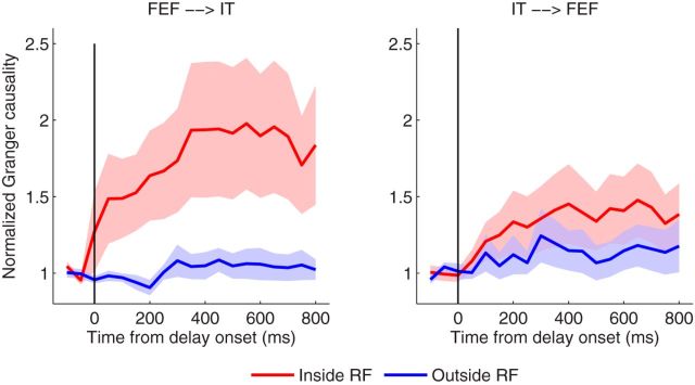
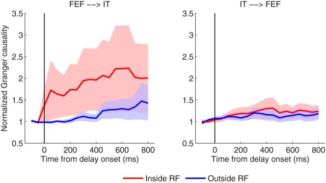
We next examined the causal influence between the FEF and IT, measured by the Granger causality, to assess the functional role of the FEF in the selection and retention of visual information in working memory. When we fitted the model to the spikes with the bin size of 1 ms, the model order of 6, as determined by AIC, was selected for both the copula GLM and marginal GLM. We have analyzed 26 pairs of neurons between FEF and the preferred IT, and 22 pairs of neurons between FEF and the nonpreferred IT. For each pair, we had 30 trials in average, and then performed statistic tests across pairs. In total, we had >1200 trials analyzed. Our first set of analysis was to compare conditions (1) with (2), where the sample object was always preferred for the IT neurons. Granger causality analysis was performed on the spike trains from FEF and IT for each trial. A 400 ms long sliding window with a step of 50 ms was used to monitor the dynamic functional interactions during the memory task. As shown in Figure 9, left, there exists significant Granger causality in FEF→IT direction starting ∼100 ms following the delay (p < 0.05, one-tail t test) when compared with the neurons inside RF to those outside RF. However, the opposite direction in IT→FEF (Fig. 9, right) does not reveal significant Granger causality. Our statistical test can be further strengthened (p = 0.0064) by combining multiple time windows using the test statistic of the maximum mean discrepancy (Gretton et al., 2012). A two-way ANOVA (directionality and RF location) was subsequently performed, which showed the significant difference in directionality (p < 0.05) during the time period from 100 to 400 ms following the delay. We note that, when determining the mode order, there is no clear “elbow” in the AIC curve for the neural data; selecting a model order slightly different from 6 does not change the conclusions. We also note the use of the 400 ms long window during which it assumed that the neuron fires at a constant background rate. Given the low firing rate of baseline in our data (e.g., Fig. 8E), such an assumption seems to be a plausible approximation. However, in the presence of strong nonstationarity in spike trains, methods to account for time-varying trial-to-trial variation should be considered to improve the estimation and inference (Ventura et al., 2005; Kelly and Kass, 2012).

Figure 9.

Comparison of Granger causality obtained via the copula GLM model between conditions (Inside vs Outside) in the direction of FEF→IT (left) and IT→FEF (right), where the sample image is always preferred for IT neurons. Note that data are standardized by the sample period to compare the causal influence in different conditions. Error bars denote the SEM. It is clearly seen that the Granger causality in FEF→IT shows a clear separation between two conditions, but not for the opposite direction in IT→FEF.

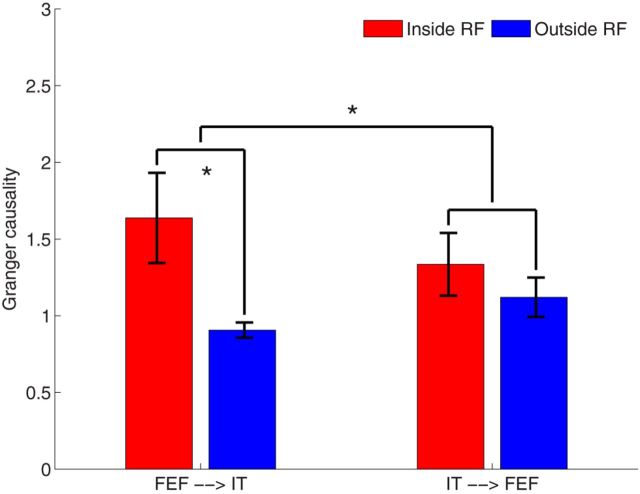
Figure 10 provides an example to show the ANOVA test result at the time of the 200 ms. It is evident that the Granger causality in the direction of FEF→IT has significant difference between two conditions (inside RF vs outside RF), and the effect is significantly larger than that in the opposite direction of IT→FEF. These results indicate that spatial selection in FEF precedes object identification in IT during memory task. The findings are further supported by directly comparing the response of FEF neurons to that of IT neurons when a sample object appears inside the FEF RF and is preferred for the IT neurons (Fig. 8E), where the FEF neurons fire earlier than the IT neurons.

Figure 10.

ANOVA test for the interaction between directionality (FEF→IT vs IT→FEF) and experimental conditions (Inside vs Outside), *p < 0.05. The asterisk on the left denotes significantly different (p = 0.0232) Granger causalities between conditions in the direction of FEF→IT, whereas the asterisk on the right denotes that the experimental effect is significantly different (p = 0.0390) in two directions (FEF→IT vs IT→FEF).

In comparison, we also applied the marginal GLM to the same data. The results are shown in Figure 11, where we observed that the Granger causality derived from the marginal GLM yields a similar trend to our method, but does not reveal significant causal influence in both directions and conditions.

Figure 11.

Comparison of Granger causality obtained via the marginal GLM model. We see that the marginal GLM fails to reveal significant causal influence in the direction of FEF→IT. Data are presented as in Figure 9.

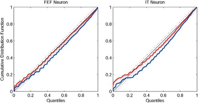
To assess the GOF of the estimated model (Brown et al., 2002), we performed the KS plots. Specifically, we used the time-rescaling theorem to transform neural spike train data to a continuous measure suitable for a GOF assessment (Brown et al., 2002). With the estimated CIF, we can compute the rescaled times. Under the assumption of model correctness (i.e., the estimated CIF provides a good approximation to the true conditional intensity of the spike trains), these rescaled times should follow the uniform distribution on the interval (0, 1]. We can visualize the result with the KS plot by sorting the rescaled times against the quantiles of the cumulative distribution function of the uniform distribution on (0, 1]. A 45 degree line in the KS plot represents exact agreement between the model and spike train data. We can use the distribution of the KS statistic to build the 95% confidence bounds for the degree of agreement between the model and the data. This procedure was done for all the neurons in the study. Most KS plots (23/26) were almost within the confidence intervals, indicating overall a good fit to the data. Fig. 12 shows examples of the KS plots obtained using the proposed copula GLM model (red) and the marginal GLM model (blue) for an FEF neuron (left) and an IT neuron (right). It is clear that our copula-based approach has a better GOF than the marginal GLM model.

Figure 12.

Comparison of the KS plots between the copula GLM model (red) and the marginal GLM model (blue) for an FEF neuron (left) and an IT neuron (right). The 45 degree blue line denotes exact agreement between the model and spike train data, with the 95% confidence bounds indicated by the flanking dashed lines.

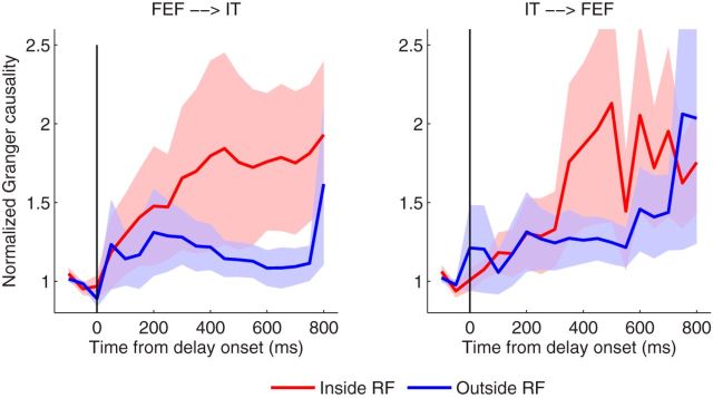
Similar to the above analysis procedure, we conducted our second set of analysis by comparing conditions (3) with (4), where the sample object is always nonpreferred for the IT neurons. The results are shown in Figure 13, where no significant causal influence was observed in either direction. This result is not unexpected because the IT neurons under such experimental conditions become less active due to the nonpreferred object. As such, there is no significant information transfer observed between FEF and IT during the delay period of the memory task.

Figure 13.

Comparison of Granger causality obtained via the copula GLM model between conditions (Inside vs Outside) in the direction of FEF→IT (left) and IT→FEF (right), where the sample image is always not preferred for IT neurons. Note that data are standardized by the sample period to compare the causal influence in different conditions. Error bars denote the SEM. There is no significant causal influence observed in either direction.

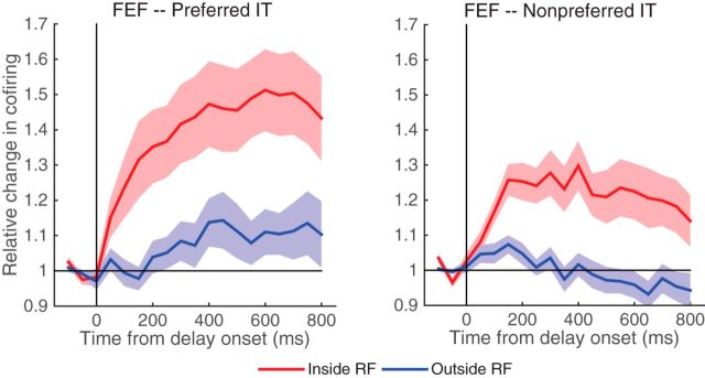
Our copula GLM can attend to both sequential dependence and shared influences on spike activity. Thus far, we have demonstrated that the time-lagged dependence can be measured by Granger causality influence with our model. We show next that the synchronous spiking can be assessed by the Gaussian copula parameter r. This can be achieved via computing the Kendall's tau (Song, 2007), which is a common metrics for measuring the degree of the dependence as it can be related to different parameters in various copulas. To make it interpretable, we normalize the Kendall's tau against the baseline to indicate the deviation of cofiring from independence. Figure 14 shows an example of the relative changes in joint firing between FEF and IT neurons, where the FEF neurons inside RF are compared with those outside RF, but for the IT neurons the sample object is always preferred (Fig. 9, left). We observe from Figure 14, left, that the synchronous spiking for FEF neurons inside RF is significantly larger than neurons outside RF starting 100 ms (p < 0.05) following the delay. In comparison, we also compute the synchronous spiking for the nonpreferred IT neurons (Fig. 13, left). It is intriguing that a similar effect is observed for the nonpreferred IT neurons (Fig. 14, right). While these results clearly indicate that FEF and IT neurons tend to fire more synchronously after the delay onset, the synchronous spiking might not be sensitive to distinguish whether the IT neurons are preferred or not.

Figure 14.

Comparison of synchronous spiking, as measured by the relative change in cofiring to the baseline, between FEF and IT neurons between conditions (Inside vs Outside RF) where the sample object is preferred (left) and nonpreferred (right) for the IT neurons.

Discussion

In this paper, we have introduced a flexible, statistically accurate, and copula-based joint GLM framework to model a multivariate point process capable of capturing not only the lagged dependence of spiking activity from individual neurons but also the contemporaneous dependence among multiple neurons. Utilizing the likelihood method, we developed (1) a maximum likelihood parameter estimation procedure that was implemented by a Gauss–Newton type algorithm and (2) a Granger causality measure for the analysis of neural spike trains. Our method was validated by extensive simulations, and compared favorably to the widely used marginal GLMs. We also demonstrated the effectiveness of our method in the analysis of spike train data simultaneously collected from both FEF and IT neurons of a monkey performing an object-based working memory task.

Compared with the popular marginal GLMs (Truccolo et al., 2005), our joint regression analysis has several advantages. First, it is a general method that can capture both history dependency and joint dependency of neural responses, which is unique for our method to explicitly model simultaneous occurrences of spike events with a copula. Second, it is flexible to handle different dependence structures specified by different copulas, thus allowing better description of neural dependencies. Third, the joint analysis results in more accurate estimation of regression coefficients than the marginal GLMs. Finally, it is straightforward to show that Granger causality between neural spike trains can be readily assessed via the likelihood ratio statistic.

So far, there have been only a few applications of the copula to neural data analysis. In the analysis of spike train data, the distribution of the first-spike latency has been used to estimate the conditional entropy of neural responses (Jenison and Reale, 2004). The neural dependencies have been characterized by copula models based on the distribution of either the spike counts (Berkes et al., 2009) or the interspike intervals (Sacerdote et al., 2012; Hu et al., 2015). A recent study has shown that the synchronous spiking among multiple neurons can be detected using the copula model, whereby the parameters in the model can be estimated within a semiparametric Bayesian framework (Shahbaba et al., 2014). Recently, a copula-based Granger causality measure has been developed for a continuous time series of field potentials to capture nonlinear and high-order moment causality in the neural data (Hu and Liang, 2014). We note that our proposed copula-based joint GLM is directly applied to the neural point process itself, i.e., sequences of spike times, rather than the spike counts, which otherwise would distort the properties of spike trains and introduce spurious effects.

In the process of developing our copula-based joint GLM method, we have mainly used the Gaussian copula due to its scalability and its flexible dependence structure (Song, 2007). In practice, the dependence structures underlying the data are usually unknown and sometimes can be even complicated, and other copulas than the Gaussian copula may be preferred. In this case, the model selection procedure has to be invoked to choose the copula that best fits the data. In general, it is easy to work with bivariate copulas; yet it is rather difficult to estimate copula, particularly in higher dimensions. The Gaussian copula is an exception (Nelsen, 2006) due to its tractability analytically. The ability of estimating the Gaussian copula in higher dimensions renders our copula GLM computationally feasible for multiple neurons, which allows us to examine the potential multi-neuron dependence due to shared inputs and network activity (Kelly et al., 2010; Kelly and Kass, 2012). We note, however, that it is usually not common to observe both the time-lagged effect and synchronous firing among more than three neurons.

In our copula-based joint GLMs, we derive a simultaneous maximum likelihood procedure for parameter estimation. There are a couple of options to evaluate the uncertainty of the maximum likelihood estimator. The classical approach is to approximate the variances of the estimated parameters by the observed Fisher information. Under standard regularity conditions, the maximum likelihood estimator will be consistent and asymptotically normal with the covariance matrix given by the Fisher information, which is the negative of the second derivative (the Hessian matrix, H(θ) = ∇²ℓ(θ)) of the log-likelihood function. A more robust approach that has been spurred by the increasing presence of multidimensional data that potentially exhibit non-normal features such as heavy tails and multimodality is to consider the possible misspecifications of the model, where the asymptotic variance can be estimated by the inverse of the Godambe information (Godambe, 1991), also known as the robust sandwich-type estimate (Song, 2007), I(θ) = H⁻¹(θ)B_n(θ)H⁻¹(θ). Moreover, the widespread BFGS optimization algorithm (or quasi-Newton algorithm) returns an approximation of the Hessian matrix that is obtained via numerical derivatives. In our implementation, we use the unconstrained nonlinear optimization algorithm (the MATLAB function fminunc) for parameter optimization, which also provides a numerical Hessian that is used to evaluate the variances of the estimated parameters. We use multiple random starts to mitigate the problem of local solutions. In addition, we assess the goodness-of-fit of the estimated model with the KS plots to check the agreement between a statistical model and the spike train data.

For continuous random variables, a copula is unique as per Sklar's Theorem. This, however, is no longer valid for discrete random variables, where the copula is only uniquely identified on the ranges of the marginals. Therefore, when the marginals are discrete, extra care is needed in making statistical inference for copula models (Genest and Neslehova, 2007). When marginal models are discrete, we adopt an approach suggested by Song (2007) where a multivariate probability mass function is obtained by taking Radon–Nikodym derivatives. We note the interpretations can be different for continuous and discrete data. For continuous marginals, the off-diagonal elements of the correlation matrix represent their linear correlation. For discrete marginals such as spike timing, it can be interpreted as the tetrachoric correlation (Dorn and Ringach, 2003).

Previous studies (Clark et al., 2012) provided evidence that FEF neurons preserve a spatially tuned persistent activity during the delay period of the DMS task, which requires maintenance of object but not spatial information. In contrast, IT neurons exhibit persistent activity that is selective for the sample identity, but not location, during DMS tasks (Chelazzi et al., 1993, 1998), but the interactions between the spatial signals in FEF and object information in IT during an object-based DMS task are not yet well understood. Our approach offers a more sensitive measure than the marginal GLM to assess directional influence between spike trains. As demonstrated by the analysis of the spiking activity simultaneously collected from FEF and IT areas during the delay period of the object-based DMS task, we found significant Granger causality influence of FEF on IT when comparing the neurons inside RF with those outside RF, and the effect is significantly larger than that in the opposite direction of IT→FEF; this result is consistent with the idea that spatial selection in FEF precedes object identification in IT during memory task. The analysis of the same data by the marginal GLM did not reveal any significant causal influence in both directions and RF conditions. These results demonstrate that our joint regression model offers a more powerful inference than separate, marginal GLM analysis.

Several extensions and improvements of this work are envisioned. First, as the number of neurons grows, efficient algorithms are needed to remain tractable for maximum-likelihood estimation. Second, the model assumes that all the neurons under consideration have the same marginal distribution, i.e., all neurons follow either the Bernoulli or Poisson distribution; thus, the model can be improved to handle different marginal distributions. Third, when analyzing spiking activity of multiple neurons, our current approach is to model each pair of neurons (one to one) by incorporating the time-lagged history information of other variables into the regression. Although this method works well in our examples, a fully high-dimensional copula model is to be developed for one-to-many, many-to-one, and many-to-many neural interactions. Finally, it is encouraging that our copula model is able to separate the dependence of neurons into two distinct parts: a lagged dependence, which measures how neurons are connected to each other, and a contemporaneous dependence, which is shared among all neurons in the network. Our proposed model, as an extension of previous work, is focused on partitioning dependence structures by including the spike-feedback terms in a generalized linear point-process model. We are therefore enthusiastic that our proposed framework will prove itself of general value in the field of neural data analysis.

References

- Akaike H. A new look at the statistical model identification. IEEE Trans Automat Contr. 1974;19:716–723. doi: 10.1109/TAC.1974.1100705. [DOI] [Google Scholar]
- Armstrong KM, Fitzgerald JK, Moore T. Changes in visual receptive fields with microstimulation of frontal cortex. Neuron. 2006;50:791–798. doi: 10.1016/j.neuron.2006.05.010. [DOI] [PubMed] [Google Scholar]
- Ba D, Temereanca S, Brown EN. Algorithms for the analysis of ensemble neural spiking activity using simultaneous-event multivariate point-process models. Front Comput Neurosci. 2014;8:6. doi: 10.3389/fncom.2014.00006. [DOI] [PMC free article] [PubMed] [Google Scholar]
- Berkes P, Wood F, Pillow J. Characterizing neural dependencies with copula models. Adv Neural Inform Process Syst. 2009;21:129–136. [Google Scholar]
- Brillinger DR. Maximum likelihood analysis of spike trains of interacting nerve cells. Biol Cybern. 1988;59:189–200. doi: 10.1007/BF00318010. [DOI] [PubMed] [Google Scholar]
- Brody CD. Correlations without synchrony. Neural Comput. 1999a;11:1537–1551. doi: 10.1162/089976699300016133. [DOI] [PubMed] [Google Scholar]
- Brody CD. Disambiguating different covariation. Neural Comput. 1999b;11:1527–1535. doi: 10.1162/089976699300016124. [DOI] [PubMed] [Google Scholar]
- Brown EN, Barbieri R, Ventura V, Kass RE, Frank LM. The time-rescaling theorem and its application to neural spike train data analysis. Neural Comput. 2002;14:325–346. doi: 10.1162/08997660252741149. [DOI] [PubMed] [Google Scholar]
- Brown EN, Barbieri R, Eden UT, Frank LM. Likelihood methods for neural data analysis. In: Feng J, editor. Computational neuroscience: a comprehensive approach. London: CRC; 2003. pp. 253–286. [Google Scholar]
- Brown EN, Kass RE, Mitra PP. Multiple neural spike train data analysis: state-of-the-art and future challenges. Nat Neurosci. 2004;7:456–461. doi: 10.1038/nn1228. [DOI] [PubMed] [Google Scholar]
- Bruce CJ, Goldberg ME. Primate frontal eye fields. I. Single neurons discharging before saccades. J Neurophysiol. 1985;53:603–635. doi: 10.1152/jn.1985.53.3.603. [DOI] [PubMed] [Google Scholar]
- Chelazzi L, Miller EK, Duncan J, Desimone R. A neural basis for visual search in inferior temporal cortex. Nature. 1993;363:345–347. doi: 10.1038/363345a0. [DOI] [PubMed] [Google Scholar]
- Chelazzi L, Duncan J, Miller EK, Desimone R. Responses of neurons in inferior temporal cortex during memory-guided visual search. J Neurophysiol. 1998;80:2918–2940. doi: 10.1152/jn.1998.80.6.2918. [DOI] [PubMed] [Google Scholar]
- Chornoboy ES, Schramm LP, Karr AF. Maximum likelihood identification of neuronal point process systems. Biol Cybern. 1988;59:265–275. doi: 10.1007/BF00332915. [DOI] [PubMed] [Google Scholar]
- Clark KL, Noudoost B, Moore T. Persistent spatial information in the frontal eye field during object-based short-term memory. J Neurosci. 2012;32:10907–10914. doi: 10.1523/JNEUROSCI.1450-12.2012. [DOI] [PMC free article] [PubMed] [Google Scholar]
- Daley DJ, Vere-Jones D. An introduction to the theory of point process. New York: Springer; 2003. [Google Scholar]
- Ding M, Chen Y, Bressler SL. Granger causality: basic theory and application to neuroscience. In: Schelter B, Winterhalder N, Timmer J, editors. Handbook of time series analysis; recent theoretical developments and applications. Berlin: Wiley; 2006. pp. 437–460. [Google Scholar]
- Dorn JD, Ringach DL. Estimating membrane voltage correlations from extracellular spike trains. J Neurophysiol. 2003;89:2271–2278. doi: 10.1152/jn.000889.2002. [DOI] [PubMed] [Google Scholar]
- Fougnie D, Marois R. Attentive tracking disrupts feature binding in visual working memory. Vis Cogn. 2009;17:48–66. doi: 10.1080/13506280802281337. [DOI] [PMC free article] [PubMed] [Google Scholar]
- Genest C, Neslehova J. A primer on copulas for count data. ASTIN Bull. 2007;37:475–515. doi: 10.2143/AST.37.2.2024077. [DOI] [Google Scholar]
- Godambe PV. Estimating functions: an overview. Oxford UP: Oxford; 1991. [Google Scholar]
- Gretton A, Borgwardt K, Rasch M, Schoelkopf B, Smola A. A kernel two-sample test. J Mach Learn Res. 2012;13:723–773. [Google Scholar]
- Gutnisky DA, Josiæ K. Generation of spatiotemporally correlated spike trains and local field potentials using a multivariate autoregressive process. J Neurophysiol. 2010;103:2912–2930. doi: 10.1152/jn.00518.2009. [DOI] [PubMed] [Google Scholar]
- He J, Li H, Edmondson AC, Rader DJ, Li M. A Gaussian copula approach for the analysis of secondary phenotypes in case-control genetic association studies. Biostatistics. 2012;13:497–508. doi: 10.1093/biostatistics/kxr025. [DOI] [PMC free article] [PubMed] [Google Scholar]
- Hu M, Liang H. A copula approach to assessing Granger causality. Neuroimage. 2014;100:125–134. doi: 10.1016/j.neuroimage.2014.06.013. [DOI] [PubMed] [Google Scholar]
- Hu M, Li W, Liang H. A copula-based Granger causality measure for the analysis of neural spike train data. IEEE/ACM Trans Comput Biol Bioinformatics. 2015 doi: 10.1109/TCBB.2014.2388311. Advance online publication. Retrieved January 1, 2015. [DOI] [PubMed] [Google Scholar]
- Jenison RL, Reale RA. The shape of neural dependence. Neural Comput. 2004;16:665–672. doi: 10.1162/089976604322860659. [DOI] [PubMed] [Google Scholar]
- Joe H. Multivariate models and dependence concepts. London: Chapman and Hall; 1997. [Google Scholar]
- Kaminski M, Liang H. Causal influence: advances in neurosignal analysis. Crit Rev Biomed Eng. 2005;33:347–430. doi: 10.1615/CritRevBiomedEng.v33.i4.20. [DOI] [PubMed] [Google Scholar]
- Kass RE, Kelly RC, Loh WL. Assessment of synchrony in multiple neural spike trains using loglinear point process models. Ann Appl Stat. 2011;5:1262–1292. doi: 10.1214/10-AOAS429. [DOI] [PMC free article] [PubMed] [Google Scholar]
- Kass RE, Eden U, Brown EN. Springer series in statistics. New York: Springer; 2014. Analysis of neural data. [Google Scholar]
- Kelly RC, Kass RE. A framework for evaluating pairwise and multiway synchrony among stimulus-driven neurons. Neural Comput. 2012;24:2007–2032. doi: 10.1162/NECO_a_00307. [DOI] [PMC free article] [PubMed] [Google Scholar]
- Kelly RC, Kass RE, Smith MA, Lee TS. Accounting for network effects in neuronal responses using L1 regularized point process models. Adv Neural Inf Process Syst. 2010;23:1099–1107. [PMC free article] [PubMed] [Google Scholar]
- Kim S, Putrino D, Ghosh S, Brown EN. A Granger causality measure for point process models of ensemble neural spiking activity. PLoS Comput Biol. 2011;7:e1001110. doi: 10.1371/journal.pcbi.1001110. [DOI] [PMC free article] [PubMed] [Google Scholar]
- Krumin M, Shoham S. Multivariate autoregressive modeling and Granger causality analysis of multiple spike trains. Comput Intell Neurosci. 2010;2010:752428. doi: 10.1155/2010/752428. [DOI] [PMC free article] [PubMed] [Google Scholar]
- Li M, Boehnke M, Abecasis GR, Song PX. Quantitative trait linkage analysis using Gaussian copulas. Genetics. 2006;173:2317–2327. doi: 10.1534/genetics.105.054650. [DOI] [PMC free article] [PubMed] [Google Scholar]
- Logothetis NK, Sheinberg DL. Visual object recognition. Annu Rev Neurosci. 1996;19:577–621. doi: 10.1146/annurev.ne.19.030196.003045. [DOI] [PubMed] [Google Scholar]
- Mishkin M, Ungerleider LG, Macko KA. Object vision and spatial vision: two cortical pathways. Trends Neurosci. 1983;6:414–417. doi: 10.1016/0166-2236(83)90190-X. [DOI] [Google Scholar]
- Moore T, Fallah M. Control of eye movements and spatial attention. Proc Natl Acad Sci U S A. 2001;98:1273–1276. doi: 10.1073/pnas.98.3.1273. [DOI] [PMC free article] [PubMed] [Google Scholar]
- Nedungadi AG, Rangarajan G, Jain N, Ding M. Analyzing multiple spike trains with nonparametric Granger causality. J Comput Neurosci. 2009;27:55–64. doi: 10.1007/s10827-008-0126-2. [DOI] [PubMed] [Google Scholar]
- Nelsen RB. An introduction to copulas. New York: Springer; 2006. [Google Scholar]
- Okatan M, Wilson MA, Brown EN. Analyzing functional connectivity using a network likelihood model of ensemble neural spiking activity. Neural Comput. 2005;17:1927–1961. doi: 10.1162/0899766054322973. [DOI] [PubMed] [Google Scholar]
- Paninski L, Ahmadian Y, Ferreira DG, Koyama S, Rahnama Rad K, Vidne M, Vogelstein J, Wu W. A new look at state-space models for neural data. J Comput Neurosci. 2010;29:107–126. doi: 10.1007/s10827-009-0179-x. [DOI] [PMC free article] [PubMed] [Google Scholar]
- Pillow JW, Shlens J, Paninski L, Sher A, Litke AM, Chichilnisky EJ, Simoncelli EP. Spatio-temporal correlations and visual signalling in a complete neuronal population. Nature. 2008;454:995–999. doi: 10.1038/nature07140. [DOI] [PMC free article] [PubMed] [Google Scholar]
- Ruppert D. Discussion of “Maximization by parts in likelihood inference.”. J Am Stat Assoc. 2005;100:1161–1163. doi: 10.1198/016214505000000240. [DOI] [Google Scholar]
- Sacerdote L, Tamborrino M, Zucca C. Detecting dependencies between spike trains of pairs of neurons through copulas. Brain Res. 2012;1434:243–256. doi: 10.1016/j.brainres.2011.08.064. [DOI] [PubMed] [Google Scholar]
- Serfling RJ. Approximation theorems of mathematical statistics. New York: Wiley; 1980. [Google Scholar]
- Shahbaba B, Zhou B, Lan S, Ombao H, Moorman D, Behseta S. A semiparametric Bayesian model for detecting synchrony among multiple neurons. Neural Comput. 2014;26:2025–2051. doi: 10.1162/NECO_a_00631. [DOI] [PMC free article] [PubMed] [Google Scholar]
- Sklar A. Random variables, joint distributions, and copulas. Kybernetica. 1973;9:449–460. [Google Scholar]
- Song PX-K. Correlated data analysis: modeling, analytics, and applications. New York: Springer; 2007. [Google Scholar]
- Song PX, Li M, Yuan Y. Joint regression analysis of correlated data using Gaussian copulas. Biometrics. 2009;65:60–68. doi: 10.1111/j.1541-0420.2008.01058.x. [DOI] [PubMed] [Google Scholar]
- Squire RF, Noudoost B, Schafer RJ, Moore T. Prefrontal contributions to visual selective attention. Annu Rev Neurosci. 2013;36:451–466. doi: 10.1146/annurev-neuro-062111-150439. [DOI] [PubMed] [Google Scholar]
- Stevenson IH, Rebesco JM, Hatsopoulos NG, Haga Z, Miller LE, Körding KP. Inferring functional connections between neurons. Curr Opin Neurobiol. 2008;18:582–588. doi: 10.1109/TNSRE.2008.2010471. [DOI] [PMC free article] [PubMed] [Google Scholar]
- Treisman A, Zhang W. Location and binding in visual working memory. Mem Cognit. 2006;34:1704–1719. doi: 10.3758/BF03195932. [DOI] [PMC free article] [PubMed] [Google Scholar]
- Truccolo W, Eden UT, Fellows MR, Donoghue JP, Brown EN. A point process framework for relating neural spiking activity to spiking history, neural ensemble, and extrinsic covariate effects. J Neurophysiol. 2005;93:1074–1089. doi: 10.1152/jn.00697.2004. [DOI] [PubMed] [Google Scholar]
- Ventura V, Cai C, Kass RE. Trial-to-trial variability and its effect on time-varying dependency between two neurons. J Neurophysiol. 2005;94:2928–2939. doi: 10.1152/jn.00644.2004. [DOI] [PubMed] [Google Scholar]
- Wood JN. When do spatial and visual working memory interact? Atten Percept Psychophys. 2011;73:420–439. doi: 10.3758/s13414-010-0048-8. [DOI] [PubMed] [Google Scholar]