

Short abstract
Methods to quantify ventricle material properties noninvasively using in vivo data are of great important in clinical applications. An ultrasound echo-based computational modeling approach was proposed to quantify left ventricle (LV) material properties, curvature, and stress/strain conditions and find differences between normal LV and LV with infarct. Echo image data were acquired from five patients with myocardial infarction (I-Group) and five healthy volunteers as control (H-Group). Finite element models were constructed to obtain ventricle stress and strain conditions. Material stiffening and softening were used to model ventricle active contraction and relaxation. Systolic and diastolic material parameter values were obtained by adjusting the models to match echo volume data. Young's modulus (YM) value was obtained for each material stress–strain curve for easy comparison. LV wall thickness, circumferential and longitudinal curvatures (C- and L-curvature), material parameter values, and stress/strain values were recorded for analysis. Using the mean value of H-Group as the base value, at end-diastole, I-Group mean YM value for the fiber direction stress–strain curve was 54% stiffer than that of H-Group (136.24 kPa versus 88.68 kPa). At end-systole, the mean YM values from the two groups were similar (175.84 kPa versus 200.2 kPa). More interestingly, H-Group end-systole mean YM was 126% higher that its end-diastole value, while I-Group end-systole mean YM was only 29% higher that its end-diastole value. This indicated that H-Group had much greater systole–diastole material stiffness variations. At beginning-of-ejection (BE), LV ejection fraction (LVEF) showed positive correlation with C-curvature, stress, and strain, and negative correlation with LV volume, respectively. At beginning-of-filling (BF), LVEF showed positive correlation with C-curvature and strain, but negative correlation with stress and LV volume, respectively. Using averaged values of two groups at BE, I-Group stress, strain, and wall thickness were 32%, 29%, and 18% lower (thinner), respectively, compared to those of H-Group. L-curvature from I-Group was 61% higher than that from H-Group. Difference in C-curvature between the two groups was not statistically significant. Our results indicated that our modeling approach has the potential to determine in vivo ventricle material properties, which in turn could lead to methods to infer presence of infarct from LV contractibility and material stiffness variations. Quantitative differences in LV volume, curvatures, stress, strain, and wall thickness between the two groups were provided.
Keywords: heart attack, infarct, ventricle model, ventricle mechanics, left ventricle
1. Introduction
Medical images and computational modeling have been used more and more in cardiovascular research [1]. Accurate evaluation of global and regional LV function is of vital importance for diagnosis, prognosis, and therapeutic options of multiple cardiovascular diseases [2–8]. Echocardiography is the main imaging modality for the assessment of LV structure and function [9–13]. In daily clinical practice, echocardiographic evaluation of regional LV function is mainly performed by visual estimation on two-dimensional echocardiographic images [14,15]. Several techniques were developed to quantify ventricle regional myocardial function, deformation, and strain rate [16–19]. Early 3D models for blood flow in the heart included Peskin's model which introduced fiber-based LV model and the celebrated immersed-boundary method to study blood flow features in an idealized geometry with fluid–structure interactions [20]. McCulloch et al., Guccione et al., and Holmes et al. have developed finite element ventricle models to investigate ventricle functions and various diseases [2–8]. A large amount of effort has been devoted to quantifying heart tissue mechanical properties and fiber orientations mostly using animal models [21–26]. Mojsejenko et al. proposed a method to estimate passive mechanical properties in a myocardial infarction using magnetic resonance imaging (MRI) and finite element simulations [27]. Hassaballah et al. introduced an inverse finite element method for determining the tissue compressibility of human LV wall [28]. Humphrey's book provides a comprehensive review of the literature [29]. Early MRI-based ventricle models were introduced by Axel and Saber et al. for mechanical analysis and investigations [30,31]. In our previous papers, patient-specific cardiac magnetic resonance imaging (CMR)-based computational right ventricle/left ventricle (RV/LV) models with fluid–structure interactions were introduced to assess outcomes of various RV reconstruction techniques with different scar tissue trimming and patch sizes [32–36]. Recent reviews can be found in Refs. [33] and [36].
In this paper, echo-based 3D LV models were introduced to quantify ventricle material properties, and to investigate morphological and mechanical stress/strain differences between ventricle with and without infarct. This will serve as a starting point to use computational models for infarct differentiation and surgical planning.
2. Methods
2.1. 3D Echo Data Acquisition.
Two groups of people were recruited to participate in this study with consent obtained (eight males, mean age 58.3 yr). The infarct group (I-Group) included five patients (P1–P5) with recent infarction. The healthy group (H-Group) included five healthy volunteers (P6–P10). Basic information and patient data are given in Table 1. Echo data acquisitions were performed at the First Affiliated Hospital of Nanjing Medical University, Nanjing, China. Standard echocardiograms were obtained using an ultrasound machine (E9, GE Mechanical Systems, Milwaukee, Wisconsin) with a 3 V probe. Patients were examined in the left lateral decubitus position, and images were acquired at end expiration in order to minimize global cardiac movement. Details of the data acquisition procedures were previously described and are omitted here [36]. Figures 1 and 2 show the echo images and reconstructed 3D LV geometries from the two group patients. The location of infarction was defined as a decrease in or cessation of myocardial contractility, which was determined by two experienced observers through visualization of all LV wall segments, combining with the electrocardiogram and results of coronary angiography. In Vivo LV pressure was recorded for modeling use (Fig. 3).
Table 1.
Patient data and ventricle volume data. I-Group: infarct group; H-Group: healthy group.
|
Pressure (mm Hg) |
Echo vol (ml) |
Model vol (ml) |
|||||||||
|---|---|---|---|---|---|---|---|---|---|---|---|
| Age | Sex | Disease | Min | Max | Min | Max | Echo EF (%) | Min | Max | Model EF (%) | |
| P1 | 60 | M | Inferior and posterior myocardial infarction | 10 | 121 | 103 | 176 | 41.48 | 102.84 | 175.79 | 41.5 |
| P2 | 72 | F | Anterior myocardial infarction | 8 | 96 | 50 | 98 | 48.98 | 50.1 | 97.78 | 48.76 |
| P3 | 73 | M | Inferior and posterior myocardial infarction, smoker | 9 | 105 | 115 | 193 | 40.41 | 114.93 | 192.73 | 40.37 |
| P4 | 71 | M | Anterior myocardial infarction, lower limb atherosclerosis | 10 | 120 | 134 | 228 | 41.23 | 133.75 | 227.84 | 41.30 |
| P5 | 58 | M | Anterior myocardial infarction, mellitus, smoker | 9 | 110 | 70 | 147 | 52.38 | 69.87 | 146.37 | 52.27 |
| I-Group mean | 66.8 | 9.2 | 110.4 | 94.4 | 168 | 44.9 | 94.3 | 168.1 | 44.8 | ||
| P6 | 48 | M | Hypertension, smoker | 9 | 115 | 46 | 116 | 60.34 | 46.01 | 115.69 | 60.23 |
| P7 | 43 | F | none | 10 | 130 | 46 | 120 | 61.67 | 45.73 | 119.58 | 61.77 |
| P8 | 59 | M | Hypertension | 10 | 118 | 33 | 79 | 58.23 | 32.94 | 78.8 | 58.2 |
| P9 | 43 | M | None | 9 | 115 | 51 | 120 | 57.5 | 50.88 | 119.83 | 57.54 |
| P10 | 56 | M | Diabetes mellitus | 10 | 138 | 46 | 121 | 61.98 | 45.92 | 120.58 | 61.92 |
| H-group mean | 49.8 | 9.6 | 123.2 | 44.4 | 111 | 59.9 | 44.3 | 110.9 | 59.9 | ||
| P-value | 0.006 | 0.397 | 0.088 | 0.012 | .040 | .0004 | 0.0120 | 0.0403 | 0.0003 | ||
Fig. 1.
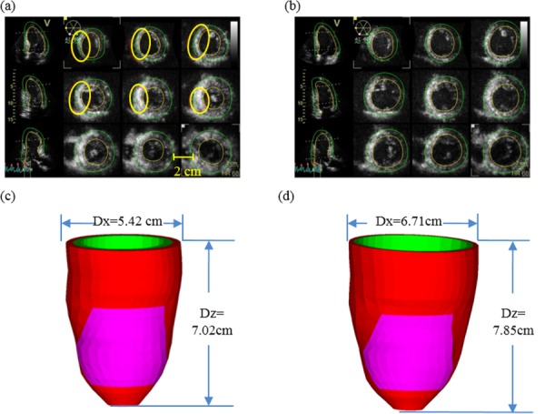
Echo images from a patient (P5) with infarct, and reconstructed geometry. Infarct locations were marked by thick circles on the echo images: (a) end-systolic echo images, (b) end-diastolic echo images, (c) reconstructed end-systolic LV geometry, and (d) reconstructed end-diastolic LV geometry
Fig. 2.
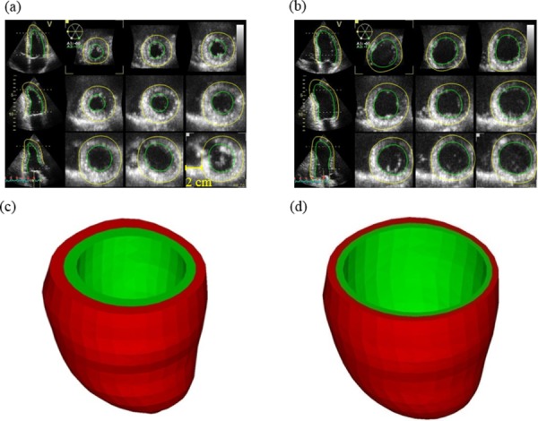
Echo images of a healthy volunteer (P6), contours and reconstructed geometries: (a) end-systolic echo, healthy volunteer, (b) end-diastolic echo, healthy volunteer, (c) reconstructed end-systolic LV geometry, and (d) reconstructed end-diastolic LV geometry
Fig. 3.
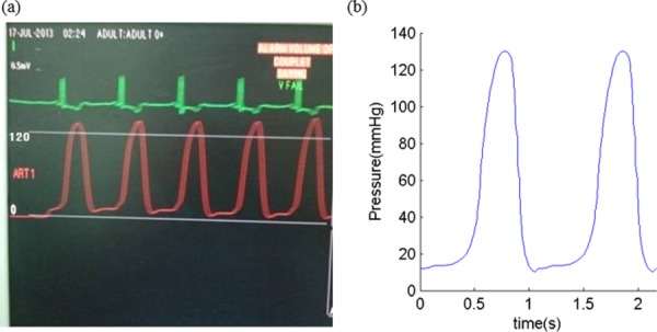
A sample of recorded and imposed LV blood pressure profile: (a) recorded LV blood pressure profile and (b) imposed LV blood pressure profile
2.2. Two-Layer Anisotropic LV Model Construction With Fiber Orientations.
The ventricle material was assumed to be hyperelastic, anisotropic, nearly incompressible and homogeneous. Infarct tissue was assumed to be hyperelastic, isotropic, nearly incompressible and homogeneous. The standard governing equations and boundary conditions for the LV model were the same as those given in Refs. [33] and [34] and are given here for easy reading
| (1) |
| (2) |
where σ is the stress tensor, ε is the strain tensor, v is displacement, and ρ is material density. Structure-only LV model was used to save model construction effort and computing time. This was adequate for our purpose in this paper to obtain LV stress/strain values for analysis.
The nonlinear Mooney–Rivlin model was available in the finite element package adina (ADINA R&D, Watertown, MA) which is the software we use to solve our models. So the Mooney–Rivlin model was used to describe the nonlinear anisotropic and isotropic material properties. The strain energy function for the isotropic Mooney–Rivlin model is given by [32–34]
| (3) |
where I 1 and I 2 are the first and second strain invariants, ci and Di are material parameters chosen to match experimental measurements [26,29,34]. The strain energy function for the anisotropic modified Mooney–Rivlin model anisotropic model was obtained by adding an additional anisotropic term in Eq. (3) [32,35]
| (4) |
where = Cij (n f)i (n f)j, Cij is the Cauchy–Green deformation tensor, n f is the fiber direction, and K 1 and K 2 are material constants [35]. Choosing c 1 = 0.351 kPa, c 2 = 0, D 1 = 0.0633 kPa, D 2 = 5.3, K 1 = 1.913 kPa, K 2 = 6.00, it was shown in Ref. [35] that stress–strain curves derived from Eq. (4) agreed well with the stress–strain curves from the dog model given in Ref. [2]
| (5) |
| (6) |
where E ff is fiber strain, E cc is cross-fiber in-plane strain, E rr is radial strain, and E cr, E fr, and E fc are the shear components in their respective coordinate planes, C, b 1, b 2, and b 3 are parameters to be chosen to fit experimental data. For simplicity, b 1, b 2, and b 3 in Eq. (6) were kept as constants, time-dependent parameter values C(t) in Eq. (5) were chosen to fit echo-measured LV volume data. Active contraction and expansion of myocardium were modeled by material stiffening and softening in our model. The stress–stretch curves and parameter values of the LV and infarct tissues are reported in Sec. 2.3.
As patient-specific fiber orientation data were not available from these patients, we chose to construct a two-layer LV model and set fiber orientation angles using fiber angles given in Ref. [29]. Fiber orientation can be adjusted when patient-specific data becomes available [37]. Figure 4 shows ventricular fiber orientations on epicardium and endocardium layers from human and a pig hearts and fiber orientations marked on the two-layer LV model corresponding to end-systole and end-diastole conditions [32–35].
Fig. 4.
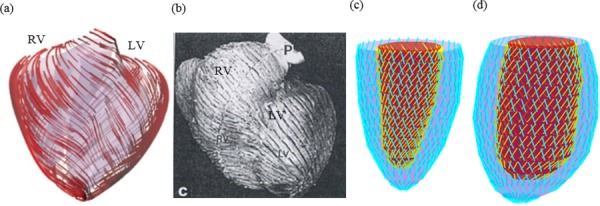
Modeling fiber orientation: (a) fiber orientation from a pig model; (b) fiber orientation from a human heart; (c) fiber orientation from our two-layer LV model, end-systolic; and (d) end-diastolic condition
2.3. A Preshrink Process and Geometry-Fitting Technique for Mesh Generation.
Under in vivo condition, ventricles were pressurized and the no-load (under zero pressure) ventricular geometries were not known. In our model construction process, a preshrink process was applied to in vivo end-systolic ventricular geometries to generate the no-load starting geometry for the computational simulation. We start with initial guesses of shrinkage rates and material parameter values, construct the model, and apply the LV minimum pressure to see if the pressurized LV volume matches in vivo LV volume data. If not, we adjust the material parameter values, pressurize it, and check again. The process is repeated until LV volume matches in vivo data with error < 0.01 cm3. Initial shrinkage was needed so that when the end-systolic pressure was applied, the ventricles would regain its in vivo morphology. The short-axis shrinkage was larger because the ventricle expanded mostly in the short-axis direction. Without this shrinking process, if we started from the in vivo end-systolic LV geometry, the ventricle would expand under pressure and its volume would be greater than the acquired in vivo end-systolic ventricle volume leading to large computational errors. The effect of the preshrink process was demonstrated by Fig. 5 [36].
Fig. 5.
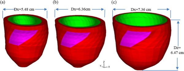
LV geometries corresponding to no-load, end-systolic, and end-diastolic conditions: (a) no-load geometry, (b) end-systolic geometry, and (c) end-diastolic geometry
A geometry-fitting mesh generation technique we developed in our previous studies was used to generate mesh for our models [24]. Using this technique, the 3D LV domain was divided into many small “volumes” to curve-fit the irregular ventricle geometry with the infarct tissue as an inclusion. Mesh analysis was performed by decreasing mesh size by 10% (in each dimension), until solution differences were less than 2%. The mesh was then chosen for our simulations.
2.4. Modeling Active Contraction and Expansion by Material Stiffening and Softening.
Modeling active LV contraction and relaxation is very difficult, and some simplifications are needed to obtain proper models to serve our purposes: (a) quantify material properties under maximum and minimum pressure conditions; (b) compare morphological and mechanical stress/strain parameter values under maximum and minimum pressure conditions. Actual LV contraction and expansion involve two different RV zero-stress geometries (diastole and systole) and interconnected changes of LV volume, pressure, stress/strain, and imposed active stress or active material properties. A cardiac cycle consists of four phases (phases 1 and 2 = systole; phases 3 and 4 = diastole):
Phase 1. Isovolumic contraction: Both mitral (inlet) and aortic (outlet) valves are closed; LV volume has no change; zero-stress sarcomere length (SL) shortens (changing from diastole zero-stress length to systole zero-stress length); however, this sarcomere shortening is not physically observable, i.e., apparent (observable) SL does not change; active stress kicks in and LV stress/strain to peak; increased stress pushes pressure to maximum.
Phase 2. Ejection: Aortic valve opens up and ejection starts; LV volume drops; strain decreases and apparent SL shortens; pressure drops; stress drops; at end of systole, LV volume reaches its minimum.
Phase 3. Isovolumic relaxation: Aortic valve closes (both valves closed); zero-stress SL relaxes from systole zero-stress length to diastole zero-stress length (noncontracted length); apparent SL does not change since LV volume does not change; strain and stress decrease to minima; pressure drops to minimum.
Phase 4. Filling: Mitral valve opens; LV volume increases to its maximum (end of diastole); pressure increases; apparent SL expands; strain and stress increases. Phase 1 will follow when filling ends.
It is very difficult to model the two isovolumic phases when the ventricle zero-stress geometry, pressure, stress, and strain are changing without volume change. For simplicity, we combined the four phases into two simplified phases [33]: (a) the filling phase when LV volume and pressure increase from their minima to their maxima. This is the combination of phases 4 and 1 given above; (b) the ejection phase when LV volume and pressure decrease from their maxima to their minima. This is the combination of phases 2 and 3 given above. Active contraction and expansion were modeled by material stiffening during contraction and material softening during expansion. Stiffening the material leads to increased stress in the strain energy function. This is actually similar to adding an active stress in other active contraction models.
Since the two isovolumic phases were omitted in our two-phase filling–ejection model, RV volume, pressure, stress, and strain achieve their minima and maxima at BF and BE, respectively. This simplified our modeling effort considerably. By omitting the two isovolumic phases, end-systolic and end-diastolic were made equivalent to BF and BE and used equally in this paper. They should be understood with our model assumptions.
Material stiffening and softening were achieved by adjusting parameter values at each echo-time step (28 echo frames per cycle) to simulate active contraction and expansion and match LV volume data. For simplicity, we set b 1 = 0.8552, b 2 = 1.7005, and b 3 = 0.7742 in Eq. (6) so that we can have a single parameter C for comparison. The least-squares method was used to find the equivalent YM for the material curves for easy comparison.
2.5. Solution Methods and Simulation Procedures.
The anisotropic LV computational models were constructed for the two groups, and the models were solved by adina (ADINA R&D, Watertown, MA) using unstructured finite elements and the Newton–Raphson iteration method. Stress/strain distributions were obtained for analysis.
2.6. Ventricle Wall Thickness and Curvature Calculation, Data for Statistical Analysis.
For each LV data set (11 slices, slices are short-axis cross sections), we divided each slice into four quarters, each quarter with equal inner wall circumferential length. Ventricle wall thickness, circumferential curvature (C-curvature), longitudinal curvature (L-curvature), and stress/strain were calculated at all nodal points (100 points/slice, 25 points/quarter). Since stress and strain are tensors, the maximum principal stress and strain were used as the representative scalar values for stress and strain at each node, respectively. The “quarter” values of those parameters were obtained by taking averages of those quantities over the 25 points for each quarter and saved for analysis. The quarter values of those from the two patients were compared to see if there are any statistically significant differences.
C-curvature (κ c) at each point on a LV inner surface slice contour was calculated using
| (7) |
where each contour is a planar curve, (x,y) are coordinates of points on the contour, and the derivatives were evaluated using neighboring points on the contour. L-curvature (κ) at each point on a LV inner contour was calculated using
| (8) |
where the longitudinal curve is given by X = (x(t), y(t), z(t)), the derivatives were evaluated using points from neighboring slices vertically below and above the point being considered.
2.7. Statistical Analysis.
All LV wall thickness, volume, ejection fraction (EF), C- and L-curvature, and stress and strain data were collected, and standard correlation analyses and Student t-test were performed for possible correlations and group differences.
3. Results
3.1. Echo-Based Models Were Able to Estimate In Vivo LV Material Parameter Values.
Human ventricle tissue material properties are extremely hard to get noninvasively under in vivo conditions. With patient-specific echo ventricle morphological data and the corresponding recorded pressure conditions, we were able to determine parameter values in the Mooney–Rivlin models in Eqs. (3), (5), and (6). Using the fiber coordinates and Eq. (6), end-systole and end-diastole LV material parameter values for the two groups are given in Table 2. Figure 6 gives the stress–stretch plots for two patients, one from each group for illustration. Using the mean value of healthy group (H-Group) as the base value, at end-diastole, the mean infarct group (I-Group) YM value for the fiber direction (YMf) was 54% stiffer than that of the healthy group (136.24 kPa versus 88.68 kPa). At end-systole, the mean YM values from the two groups were similar (175.84 kPa versus 200.2 kPa). More interestingly, while H-Group end-systole YMf was 126% higher that its end-diastole value, I-Group end-systole YMf was only 29% higher that its end-diastole value. This indicated that H-Group ventricles had much better contractibility reflected by greater material stiffness variations.
Table 2.
LV material parameter values. YMc:YM in circumferential direction.
| C (kPa) | YMf (kPa) | YMc (kPa) | C (kPa) | YMf (kPa) | YMc (kPa) | |
|---|---|---|---|---|---|---|
| End of diastole | End of systole | |||||
| P1 | 6.6748 | 191.1 | 66.4 | 7.7572 | 223 | 77.1 |
| P2 | 5.9532 | 171.2 | 59.2 | 7.216 | 207.5 | 71.7 |
| P3 | 3.6982 | 106.3 | 36.8 | 4.3296 | 124.5 | 43.1 |
| P4 | 2.5256 | 72.6 | 25.1 | 2.7962 | 80.4 | 27.8 |
| P5 | 4.8708 | 140 | 48.4 | 8.4788 | 243.8 | 84.3 |
| I-Group mean | 136.24 | 47.18 | Mean | 175.84 | 60.8 | |
| P6 | 2.5256 | 72.6 | 25.1 | 6.6748 | 191.9 | 66.4 |
| P7 | 2.5256 | 72.6 | 25.1 | 7.5768 | 217.8 | 75.3 |
| P8 | 3.7884 | 108.9 | 37.7 | 6.8552 | 197.1 | 68.2 |
| P9 | 4.059 | 116.7 | 40.4 | 6.8552 | 197.1 | 68.2 |
| P10 | 2.5256 | 72.6 | 25.1 | 6.8552 | 197.1 | 68.2 |
| H-Group mean | 88.68 | 30.68 | Mean | 200.2 | 69.26 | |
| P (t-test) | 0.07889 | 0.07929 | 0.46321 | 0.46098 | ||
Fig. 6.
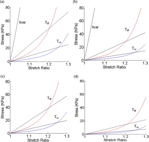
Material stress–stretch curves (in fiber coordinate) for P5 (infarct group) and P6 (healthy group). T ff: stress in fiber direction and T cc: stress in circumferential direction of the fiber: (a) P5, end-systole, (b) P5, end-diastole, (c) P6, end-systole, and (d) P6, end-diastole.
3.2. Correlations Between EF With Ventricle Morphological and Stress/Strain Conditions.
Correlations between LVEF and wall thickness, circumferential and longitudinal curvature, stress and strain values for each patient are given in Table 3. Because stress and strain are tensors, maximum principal stress and strain were used as their scalar representatives in this paper. At BE (LV pressure and volume at maximum), LVEF showed positive correlation with circumferential curvature (C-curvature), stress and strain (r = 0.7000, 0.8517, and 0.9763), and negative correlation with LV volume (r = −0.7848), respectively. At BF (LV pressure and volume at minimum), LVEF showed positive correlation with C-curvature, strain (r = 0.8097, 0.6505), but negative correlation with stress and LV volume (r = −0.9201, −0.8961), respectively. LVEF showed no significant correlation with wall thickness and L-curvature.
Table 3.
Correlations between EF and mean values of morphological and stress/strain parameters. WT: wall thickness; C-cur: C-curvature; L-cur: L-curvature; and Vol: volume. Boldfaced values indicated significant correlations.
| EF (%) | WT (cm) | C-cur (1/cm) | L-cur (1/cm) | Stress (kPa) | Strain | Vol (ml) | |
|---|---|---|---|---|---|---|---|
| BE | |||||||
| I-Group | 41.5 | 0.5488 | 0.4408 | 0.3449 | 247.6 | 0.6478 | 175.79 |
| 48.76 | 0.5651 | 0.6550 | 0.6324 | 194.1 | 0.7861 | 97.78 | |
| 40.37 | 0.6052 | 0.4278 | 0.3175 | 174.7 | 0.6425 | 192.73 | |
| 41.30 | 0.7628 | 0.4160 | 0.3642 | 176.6 | 0.5329 | 227.84 | |
| 52.27 | 0.5649 | 0.4942 | 0.5435 | 239.7 | 0.7740 | 146.37 | |
| H-Group | 60.23 | 0.7562 | 0.5642 | 0.2548 | 337.3 | 1.0323 | 115.69 |
| 61.77 | 0.6110 | 0.6030 | 0.2570 | 413.0 | 1.0483 | 119.58 | |
| 58.2 | 0.7134 | 0.7904 | 0.3483 | 280.6 | 0.9985 | 78.8 | |
| 57.54 | 0.7495 | 0.6196 | 0.2470 | 275.3 | 0.9755 | 119.83 | |
| 61.92 | 0.6853 | 0.5949 | 0.2348 | 432.7 | 1.0820 | 120.58 | |
| r | 0.3495 | 0.7002 | −0.3797 | 0.8517 | 0.9763 | −0.7848 | |
| p | 0.3223 | 0.0241 | 0.2792 | 0.0018 | 1.17E−06 | 0.0072 | |
| BF | |||||||
| I-Group | 41.5 | 0.6331 | 0.5588 | 0.3870 | 8.852 | 0.1738 | 102.84 |
| 48.76 | 0.6914 | 0.8516 | 0.5968 | 4.848 | 0.2081 | 50.10 | |
| 40.37 | 0.7129 | 0.5427 | 0.3215 | 6.715 | 0.1969 | 114.93 | |
| 41.30 | 0.9126 | 0.4985 | 0.4016 | 7.645 | 0.1670 | 133.75 | |
| 52.27 | 0.6895 | 0.7146 | 0.5410 | 5.488 | 0.1608 | 69.87 | |
| H-Group | 60.23 | 0.9816 | 0.8062 | 0.3597 | 3.494 | 0.2158 | 46.01 |
| 61.77 | 0.8040 | 0.8759 | 0.2889 | 3.803 | 0.2078 | 45.73 | |
| 58.2 | 0.9003 | 1.1392 | 0.3642 | 3.193 | 0.2080 | 32.94 | |
| 57.54 | 0.9709 | 0.8781 | 0.2743 | 3.249 | 0.2076 | 50.88 | |
| 61.92 | 0.9166 | 0.8682 | 0.3103 | 3.394 | 0.2115 | 45.92 | |
| r | 0.5847 | 0.8097 | −0.3240 | −0.9201 | 0.6505 | −0.8961 | |
| p | 0.0759 | 0.0045 | 0.3610 | 0.0002 | 0.0417 | 0.0005 | |
3.3. Infarcted LV Had Lower Stress/Strain and Thinner Wall at BE.
Comparison of LV quarterly averaged wall thickness, circumferential and longitudinal curvature, stress and strain values are given in Table 4. Figure 7 shows stress and strain plots from two patients, one from each group, to illustrate stress/strain distribution patterns.
Table 4.
Comparison of quarter mean values of ventricle wall thickness, circumferential curvature, longitudinal curvature, and mechanical stress/strain between I-Group and H-Group. Qts, quarters; WT, wall thickness; C-Cur, circumferential curvature; L-Cur, longitudinal curvature; and Stdev, standard deviation.
| Qts | WT (cm) | C-Cur (1/cm) | L-Cur (1/cm) | Stress (kPa) | Strain | |
|---|---|---|---|---|---|---|
| BE | ||||||
| I-Group (220Qts) | Mean | 0.5745 | 0.4934 | 0.4325 | 237.42 | 0.7331 |
| Stdev | 0.1209 | 0.3085 | 0.3051 | 72.36 | 0.2158 | |
| H-Group (220Qts) | Mean | 0.7031 | 0.6344 | 0.2684 | 347.77 | 1.0273 |
| Stdev | 0.1630 | 0.4720 | 0.1933 | 87.90 | 0.1285 | |
| P-value | 2.33E−06 | 0.0667 | 0.00091 | 5.55E−11 | 3.66E−14 | |
| BF | ||||||
| I-Group (220Qts) | Mean | 0.6867 | 0.6406 | 0.4461 | 7.47 | 0.2276 |
| Stdev | 0.0974 | 0.3812 | 0.2661 | 3.05 | 0.1175 | |
| H-Group (220Qts) | Mean | 0.9147 | 0.9135 | 0.3195 | 3.43 | 0.2101 |
| Stdev | 0.1393 | 0.6401 | 0.3027 | 0.70 | 0.0375 | |
| P-value | 9.526E−20 | 0.00778 | 0.0174 | 3.427E−16 | 0.29328 | |
Fig. 7.
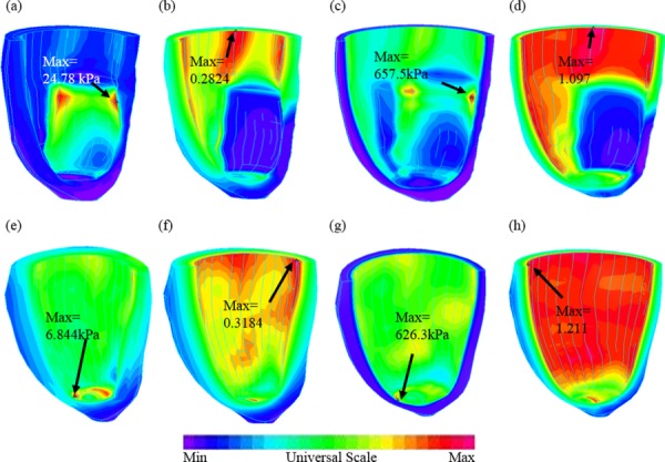
Stress-P1 (maximum principal stress) and strain-P1 (maximum principal strain) plots from P5 (with infarct) and P6 (healthy) showing stress/strain distribution patterns corresponding to maximum and minimum pressure conditions: (a) P5, stress-P1, BF; (b) P5, strain-P1, BF; (c) P5, stress-P1, BE; (d) P5, strain-P1, BE; (e) P6, stress-P1, BF; (f) P6, strain-P1, BF; (g) P6, stress-P1, BE; and (h) P6, strain-P1, BE
Among the five parameters, longitudinal curvature (L-curvature) and LV stress showed largest differences. At BE when LV volume, pressure, stress and strain were at their maxima, I-Group stress, strain, and wall thickness were 32%, 29%, and 18% lower (thinner), respectively, compared to those of H-Group. L-curvature from I-Group was 61% higher than that from H-Group. Difference in C-curvature between the two groups was not statistically significant.
At BF when LV volume, pressure, stress, and strain are at their minima, I-Group stress and L-curvature were 118% and 39.6% higher, respectively, than those of H-Group. Wall thickness and C-curvature from I-Group were 25% and 30% thinner (lower) than those from H-Group. Difference in strain between the two groups was not statistically significant.
3.4. Sensitivity Analysis and Impact of the Model Assumptions.
Sensitivity analysis was performed to study impact of model assumptions. P5 was used to make four models to demonstrate differences caused by changing one model conditions. For simplicity, the base model of patient P5 is referred to as P5. Model P5-1 is the same as P5 except that we dropped the preshrinking process, i.e., the in vivo LV geometry corresponding to minimum pressure was used as the no-load geometry to construct the model. Model P5-2 is the same as P5 except that we treated the infarct part as normal tissue. Model P5-3 was made by changing maximum pressure in P5 from 110 mm Hg to 140 mm Hg, keeping other conditions the same. In Model P5-4, parameter C value was increased by 50% to find the impact of material stiffness on model outcome. Model comparisons are given by Table 5 showing impact of model assumptions on calculated model LVEF and stress/strain outcome. Without preshrink, P5-1 led to a 42% over-estimate of LV volume at BE. Treating infarct as normal tissue also led to increased LV volume (18%) and stress/strain level (25%/17%). A 30 mm Hg pressure increase led to only a small LV volume increase (2.5%), but a considerable increase in stress (37.3%). Strain increase was only 5.2%. A 50% increase in stiffness coefficient C led to decrease of LV volume (−6.6%), decrease of stress (−14.4%), and strain (−8.3%).
Table 5.
Model comparisons showing impact of model assumptions on stress/strain outcome. Remark: BE corresponds to maximum LV pressure and volume.
|
Pressure (mm Hg) |
Echo vol (ml) |
Model vol (ml) |
|||||||
|---|---|---|---|---|---|---|---|---|---|
| Min | Max | Min | Max | Min | Max | Model EF (%) | BE mean stress (kPa) | BE mean strain | |
| P5 | 9 | 110 | 70 | 147 | 69.87 | 146.37 | 52.27 | 239.7 | 0.7740 |
| P5-1 | 9 | 110 | 70 | 147 | 99.34 | 208.31 | 52.31 | 236.7 | 0.7647 |
| P5-2 | 9 | 110 | 70 | 147 | 76.70 | 173.30 | 55.74 | 301.3 | 0.9092 |
| P5-3 | 9 | 140 | 70 | 147 | 69.87 | 153.17 | 54.38 | 329.2 | 0.8147 |
| P5-4 | 9 | 110 | 70 | 147 | 63.85 | 136.73 | 53.30 | 205.1 | 0.7102 |
4. Discussion
4.1. In Vivo Image-Based Models: What Do We Know and What Do We Want to Know.
Since it is highly risky, and often impossible, to use direct surgical approach to investigate ventricle cardiac functions and evaluate impact of different therapies, computational models have been used to perform simulations to test out feasibilities of surgical options, features of assist devices, and impact of various factors on cardiac functions [2,6,8,32]. In general, computational ventricle models require “input” information to provide accurate and reliable “output” predictions. Those input information normally include ventricle morphology, tissue material properties, fiber orientation, blood pressure, valve mechanics, active contraction information, and electric coupling. Unfortunately, when making patient-specific models using in vivo data, it is difficult to get the complete data set with desirable accuracy for the model. Patient-specific myocardium material properties are often missing in most published ventricle models. An inverse method was presented in this paper for calculating ventricle material properties based on echo image and pressure data. It should be noted that active contraction was modeled by material stiffening. No-load ventricle geometry was also determined in the process. Those made our approach unique.
4.2. Material Stiffness Parameters as Predictors of Presence of Infarct.
Identification of infarct area is of great important in clinical applications. Now that we demonstrated that ventricles with and without infarct have considerably large differences in contractibility and material stiffness variations, proper inverse methods could be introduced to determine if a ventricle had infarct based on its contractibility and material parameter values predicted by our models. This could serve as the basis for people to develop accurate and automatic methods to identify infarct area based on image data, which is of great clinical relevance.
It should be noted that our method is a “global” method in a sense that our material parameters were for the entire ventricle. Indeed, we did not have any local ventricle “tagging” information. It is beyond our method to have local property predictions.
4.3. Search for the Best Predictor for Presence of Infarct.
How to determine if a patient had infarction is of great clinical importance. Among those morphological (size, volume, wall thickness, curvature), mechanical (stiffness, stiffness variation, stress, strain), and biological (pressure, clinical symptoms) indicators, what is the best predictor for presence of infarction? Our limited study of these ten patients may provide some hint, but we could not draw any conclusion, partially because of the small size, and partially because the two groups are distinctively different. We have a long way to go to find out if the modeling approach could provide better tools to aid diagnosis or inform treatment. Basically, it is an inverse problem. First, we study enough patients to find if the two groups differ in those morphological and mechanical parameters. After we gather enough data, we ask the “reversed” questions: can we use those parameters to differentiate patients with infarct from those without? Or, can we show that some parameters have better predicting power? Large scale predictive studies are needed to get better conclusions.
We should clarify that our method would not be able to determine infarct size accurately. It would only give indication that infarct may be present. That is a hope for future application. This is to detect presence of infarct (without specific size or location information) without using more expensive imaging tools.
Several imaging techniques, such as echocardiography, MRI, and myocardial perfusion tomography are being used clinically to assess myocardial infarction. Evaluation of regional myocardial motion by echocardiography is mainly performed by visual estimation on two dimension images, which is subjective and not very reliable. Myocardial perfusion tomography is a nuclear medicine procedure that illustrates the function of myocardium. It can be used to identify location and degree of myocardial infarction. However, this technique cannot determine infarct size precisely, especially in patients with nontransmural myocardial infarction. MRI is a precise technique to quantify infarct size. But it is expensive, and the side effects of MRI contrast agent (magnetism) cannot be ignored. Besides, none of the above techniques could assess the material properties of myocardium, which is the main purpose of this paper.
4.4. Our Two-Phase Model Assumption and End-Systole/End-Diastole Terminologies.
There is a general misconception that heart contraction is kind of equal to high stress and high pressure, which is not true. Heart contraction is caused by shortening of myocardium fibers (sarcomere), which is directly related to zero-stress length of sarcomere. Heart contraction leads to high stress/high pressure during the isovolumic pre-ejection phase. When heart contract is fully realized, i.e., the heart is at its end-systole, sarcomere is at its shortest length, ventricle has its minimum volume, and stress is low, even though not at its minimum yet. Ventricle pressure and stress will continue to drop as sarcomere “relaxes,” and reach their respective minimum before mitral valve opens (prefilling). That is why we used BE and BF in this paper when end-systole and end-diastole might be misleading.
4.5. Stiffness Parameter Choices.
When adjusting material parameters in Eqs. (5) and (6) during a cardiac cycle for a given patient, we kept b 1, b 2, and b 3 as constants, and were adjusting only C value to match LV volume data. The main reason for that is we do not have data to be more specific. For most modeling research based on in vivo data, we normally work with very limited data. Theoretically, those problems are under-determined and solutions are not unique. For our paper here, the only data we have is ventricle volume. With that, we can only determine one parameter value. That is why we fixed b 1, b 2, b 3, and used volume data to determine C value. Different sets of parameter values could be used to match LV volume and they would be equally good. Still, b 1, b 2, b 3 are three numbers, it is more natural to choose C as the working parameter as our first-order approximation.
4.6. Model Limitations.
Model limitations include the following: (a) ventricle valve mechanics was not included. Valve mechanics plays an important role. However, including it will require considerable more data and modeling effort; (b) fluid–structure interaction was not included; (c) local ventricle deformation imaging data (by particle tracking) was not included; such data will be very useful for determining tissue material properties and infarct area; (d) active contraction and expansion were modeled by our two-phase model with material stiffening and softening without adjusting zero-stress ventricle geometries. Accurate zero-stress ventricle geometries are needed to further improve our models.
5. Conclusion
An echo-based computational modeling approach was proposed to investigate LV material properties and stress/strain conditions. With ten patients studied, our results indicated that our modeling approach has the potential to be used determine in vivo ventricle material properties, which in turn could lead to inverse methods to infer presence of infarct from LV contractibility and material stiffness variations. Quantitative differences in LV volume, curvatures, stress, strain, and wall thickness between the two groups were provided.
Acknowledgment
This research was supported in part by NIH-1R01-HL 089269. Chun Yang's research was supported in part by National Sciences Foundation of China No. 11171030.
Contributor Information
Longling Fan, Department of Mathematics, Southeast University, Nanjing 210096, China .
Jing Yao, Department of Cardiology, First Affiliated Hospital, of Nanjing Medical University, Nanjing 210029, China .
Chun Yang, Network Technology Research Institute, China United Network, Communications Co., Ltd., Beijing 100048, China .
Dalin Tang, School of Biological Science & Medical, Engineering, Southeast University, Nanjing 210096, China; Mathematical Sciences Department, Worcester Polytechnic Institute, Worcester, MA 01609.
Di Xu, Department of Cardiology, First Affiliated Hospital, of Nanjing Medical University, Nanjing 210029, China.
References
- [1]. Desmond-Hellmann, S. , Sawyers, C. L. , Cox, D. R. , Fraser-Liggett, C. , Galli, S. J. , Goldstein, D. B. , Hunter, D. , Kohane, I. S. , Lo, B. , Misteli, T. , Morrison, S. J. , Nichols, D. G. , Olson, M. V. , Royal, C. D. , and Yamamoto, K. R. , 2011, “Toward Precision Medicine: Building a Knowledge Network for Biomedical Research and a New Taxonomy of Disease,” Committee on a Framework for Development a New Taxonomy of Disease, National Research Council, The National Academies Press.http://www.nap.edu/catalog.php?record_id=13284 [PubMed]
- [2]. McCulloch, A. , Waldman, L. , Rogers, J. , and Guccione, J. , 1992, “Large-Scale Finite Element Analysis of the Beating Heart,” Crit. Rev. Biomed. Eng., 20(5–6), pp. 427–449. [PubMed] [Google Scholar]
- [3]. Guccione, J. M. , McCulloch, A. D. , and Waldman, L. K. , 1991, “Passive Material Properties of Intact Ventricular Myocardium Determined From a Cylindrical Model,” ASME J. Biomech. Eng., 113(1), pp. 42–55. 10.1115/1.2894084 [DOI] [PubMed] [Google Scholar]
- [4]. Guccione, J. M. , Waldman, L. K. , and McCulloch, A. D. , 1993, “Mechanics of Active Contraction in Cardiac Muscle: Part II—Cylindrical Models of the Systolic Left Ventricle,” ASME J. Biomech. Eng., 115(1), pp. 82–90. 10.1115/1.2895474 [DOI] [PubMed] [Google Scholar]
- [5]. Krishnamurthy, A. , Villongco, C. T. , Chuang, J. , Frank, L. R. , Nigam, V. , Belezzuoli, E. , Stark, P. , Krummen, D. E. , Narayan, S. , Omens, J. H. , McCulloch, A. D. , and Kerckhoffs, R. C. , 2013, “Patient-Specific Models of Cardiac Biomechanics,” J. Comput. Phys., 244, pp. 4–21. 10.1016/j.jcp.2012.09.015 [DOI] [PMC free article] [PubMed] [Google Scholar]
- [6]. Holmes, J. W. , and Costa, K. D. , 2006, “Imaging Cardiac Mechanics: What Information Do We Need to Extract From Cardiac Images?,” Conf. Proc. IEEE Eng. Med. Biol. Soc., 1, pp. 1545–1547. 10.1109/IEMBS.2006.259642 [DOI] [PubMed] [Google Scholar]
- [7]. Moyer, C. B. , Norton, P. T. , Ferguson, J. D. , and Holmes, J. W. , “Changes in Global and Regional Mechanics Due to Atrial Fibrillation: Insights From a Coupled Finite-Element and Circulation Model,” Ann. Biomed. Eng. (in press). 10.1007/s10439-015-1256-0 [DOI] [PMC free article] [PubMed] [Google Scholar]
- [8]. Fomovsky, G. M. , Macadangdang, J. R. , Ailawadi, G. , and Holmes, J. W. , 2011, “Model-Based Design of Mechanical Therapies for Myocardial Infarction,” J. Cardiovasc. Trans. Res., 4(1), pp. 82–91. 10.1007/s12265-010-9241-3 [DOI] [PMC free article] [PubMed] [Google Scholar]
- [9]. Emond, M. , Mock, M. B. , Davis, K. B. , Fisher, L. D. , Holmes, D. R., Jr. , Chaitman, B. R. , Kaiser, G. C. , Alderman, E. , and Killip, T., III , 1994, “Long-Term Survival of Medically Treated Patients in the Coronary Artery Surgery Study (CASS) Registry,” Circulation, 90(6), pp. 2645–2657. 10.1161/01.CIR.90.6.2645 [DOI] [PubMed] [Google Scholar]
- [10]. Møller, J. E. , Hillis, G. S. , Oh, J. K. , Reeder, G. S. , Gersh, B. J. , and Pellikka, P. A. , 2006, “Wall Motion Score Index and Ejection Fraction for Risk Stratification After Acute Myocardial Infarction,” Am. Heart J., 151(2), pp. 419–425. 10.1016/j.ahj.2005.03.042 [DOI] [PubMed] [Google Scholar]
- [11]. Quinones, M. A. , Greenberg, B. H. , Kopelen, H. A. , Koilpillai, C. , Limacher, M. C. , Shindler, D. M. , Shelton, B. J. , and Weiner, D. H. , 2000, “Echocardiographic Predictors of Clinical Outcome in Patients With Left Ventricular Dysfunction Enrolled in the SOLVD Registry and Trials: Significance of Left Ventricular Hypertrophy,” J. Am. Coll. Cardiol., 35(5), pp. 1237–1244. 10.1016/S0735-1097(00)00511-8 [DOI] [PubMed] [Google Scholar]
- [12]. Sabia, P. , Afrookteh, A. , Touchstone, D. A. , Keller, M. W. , Esquivel, L. , and Kaul, S. , 1991, “Value of Regional Wall Motion Abnormality in the Emergency Room Diagnosis of Acute Myocardial Infarction: A Prospective Study Using Two Dimensional Echocardiography,” Circulation, 84(3 Suppl.), pp. I85–I92. [PubMed] [Google Scholar]
- [13]. Thune, J. J. , Kober, L. , Pfeffer, M. A. , Skali, H. , Anavekar, N. S. , Bourgoun, M. , Ghali, J. K. , Arnold, J. M. , Velazquez, E. J. , and Solomon, S. D. , 2006, “Comparison of Regional Versus Global Assessment of Left Ventricular Function in Patients With Left Ventricular Dysfunction, Heart Failure, or Both After Myocardial Infarction: The Valsartan in Acute Myocardial Infarction Echocardiographic Study,” J. Am. Soc. Echocardiogr., 19(12), pp. 1462–1465. 10.1016/j.echo.2006.05.028 [DOI] [PubMed] [Google Scholar]
- [14]. Gopal, A. S. , Shen, Z. , Sapin, P. M. , Keller, A. M. , Schnellbaecher, M. J. , Leibowitz, D. W. , Akinboboye, O. O. , Rodney, R. A. , Blood, D. K. , and King, D. L. , 1995, “Assessment of Cardiac Function by Three-Dimensional Echocardiography Compared With Conventional Noninvasive Methods,” Circulation, 92(4), pp. 842–853. 10.1161/01.CIR.92.4.842 [DOI] [PubMed] [Google Scholar]
- [15]. Mondelli, J. A. , Di Luzio, S. , Nagaraj, A. , Kane, B. J. , Smulevitz, B. , Nagaraj, A. V. , Greene, R. , McPherson, D. D. , and Rigolin, V. H. , 2001, “The Validation of Volumetric Real-Time 3-Dimensional Echocardiography for the Determination of Left Ventricular Function,” J. Am. Soc. Echocardiogr., 14(10), pp. 994–1000. 10.1067/mje.2001.115770 [DOI] [PubMed] [Google Scholar]
- [16]. Edvardsen, T. , Gerber, B. L. , Garot, J. , Bluemke, D. A. , Lima, J. A. , and Smiseth, O. A. , 2002, “Quantitative Assessment of Intrinsic Regional Myocardial Deformation by Doppler Strain Rate Echocardiography in Humans: Validation Against Three Dimensional Tagged Magnetic Resonance Imaging,” Circulation, 106(1), pp. 50–56. 10.1161/01.CIR.0000019907.77526.75 [DOI] [PubMed] [Google Scholar]
- [17]. Urheim, S. , Edvardsen, T. , Torp, H. , Angelsen, B. , and Smiseth, O. A. , 2000, “Myocardial Strain by Doppler Echocardiography: Validation of a New Method to Quantify Regional Myocardial Function,” Circulation, 102(1), pp. 1158–1164. 10.1161/01.CIR.102.10.1158 [DOI] [PubMed] [Google Scholar]
- [18]. Sutherland, G. R. , Di Salvo, G. , Claus, P. , D'hooge, J. , and Bijnens, B. , 2004, “Strain and Strain Rate Imaging: A New Clinical Approach to Quantifying Regional Myocardial Function,” J. Am. Soc. Echocardiogr., 17(7), pp. 788–802. 10.1016/j.echo.2004.03.027 [DOI] [PubMed] [Google Scholar]
- [19]. Amundsen, B. H. , Helle-Valle, T. , Edvardsen, T. , Torp, H. , Crosby, J. , Lyseggen, E. , Støylen, A. , Ihlen, H. , Lima, J. A. , Smiseth, O. A. , and Slørdahl, S. A. , 2006, “Noninvasive Myocardial Strain Measurement by Speckle Tracking Echocardiography: Validation Against Sonomicrometry and Tagged Magnetic Resonance Imaging,” J. Am. Coll. Cardiol., 47(4), pp. 789–793. 10.1016/j.jacc.2005.10.040 [DOI] [PubMed] [Google Scholar]
- [20]. Peskin, C. S. , 1975, Mathematical Aspects of Heart Physiology (Lecture Notes of Courant Institute of Mathematical Sciences), New York University, New York. [Google Scholar]
- [21]. Costa, K. D. , Takayama, Y. , McCulloch, A. D. , and Covell, J. W. , 1999, “Laminar Fiber Architecture and Three-Dimensional Systolic Mechanics in Canine Ventricular Myocardium,” Am. J. Physiol., 276(2 Pt. 2), pp. H595–H607. [DOI] [PubMed] [Google Scholar]
- [22]. Nash, M. P. , and Hunter, P. J. , 2000, “Computational Mechanics of the Heart, From Tissue Structure to Ventricular Function,” J. Elasticity, 61(1–3), pp. 113–141. 10.1023/A:1011084330767 [DOI] [Google Scholar]
- [23]. Rogers, J. M. , and McCulloch, A. D. , 1994, “Nonuniform Muscle Fiber Orientation Causes Spiral Wave Drift in a Finite Element Model of Cardiac Action Potential Propagation,” J. Cardiovasc. Electrophysiol., 5(6), pp. 496–509. 10.1111/j.1540-8167.1994.tb01290.x [DOI] [PubMed] [Google Scholar]
- [24]. Sacks, M. S. , and Chuong, C. J. , 1993, “Biaxial Mechanical Properties of Passive Right Ventricular Free Wall Myocardium,” ASME J. Biomech. Eng., 115(2), pp. 202–205. 10.1115/1.2894122 [DOI] [PubMed] [Google Scholar]
- [25]. Takayama, Y. , Costa, K. D. , and Covell, J. W. , 2002, “Contribution of Laminar Myofiber Architecture to Load-Dependent Changes in Mechanics of LV Myocardium,” Am. J. Physiol. Heart Circ. Physiol., 282(4), pp. H1510–H1520. 10.1152/ajpheart.00261.2001 [DOI] [PubMed] [Google Scholar]
- [26]. Humphrey, J. D. , Strumpf, R. K. , and Yin, F. C. , 1999, “Biaxial Mechanical Behavior of Excised Ventricular Epicardium,” Am. J. Physiol., 259(1 Pt. 2), pp. H101–H108. [DOI] [PubMed] [Google Scholar]
- [27]. Mojsejenko, D. , McGarvey, J. R. , Dorsey, S. M. , Gorman, J. H., III , Burdick, J. A. , Pilla, J. J. , Gorman, R. C. , and Wenk, J. F. , 2015, “Estimating Passive Mechanical Properties in a Myocardial Infarction Using MRI and Finite Element Simulations,” Biomech. Model. Mechanobiol., 14(3), pp. 633–647. 10.1007/s10237-014-0627-z [DOI] [PMC free article] [PubMed] [Google Scholar]
- [28]. Hassaballah, A. I. , Hassan, M. A. , Mardi, A. N. , and Hamdi, M. , 2013, “An Inverse Finite Element Method for Determining the Tissue Compressibility of Human Left Ventricular Wall During the Cardiac Cycle,” PLoS One, 8(12), p. e82703. 10.1371/journal.pone.0082703 [DOI] [PMC free article] [PubMed] [Google Scholar]
- [29]. Humphrey, J. D. , 2002, Cardiovascular Solid Mechanics, Springer-Verlag, New York: 10.1007/978-0-387-21576-1 [DOI] [Google Scholar]
- [30]. Axel, L. , 2002, “Biomechanical Dynamics of the Heart With MRI,” Annu. Rev. Biomed. Eng., 4, pp. 321–347. 10.1146/annurev.bioeng.4.020702.153434 [DOI] [PubMed] [Google Scholar]
- [31]. Saber, N. R. , Gosman, A. D. , Wood, N. B. , Kilner, P. J. , Charrier, C. L. , and Firman, D. N. , 2001, “Computational Flow Modeling of the Left Ventricle Based on In Vivo MRI Data: Initial Experience,” Ann. Biomech. Eng., 29(4), pp. 275–283. 10.1114/1.1359452 [DOI] [PubMed] [Google Scholar]
- [32]. Tang, D. , Yang, C. , Geva, T. , and del Nido, P. J. , 2008, “Patient-Specific MRI-Based 3D FSI RV/LV/Patch Models for Pulmonary Valve Replacement Surgery and Patch Optimization,” ASME J. Biomech. Eng., 130(4), p. 041010. 10.1115/1.2913339 [DOI] [PMC free article] [PubMed] [Google Scholar]
- [33]. Tang, D. , Yang, C. , Geva, T. , and del Nido, P. J. , 2010, “Image-Based Patient-Specific Ventricle Models With Fluid–Structure Interaction for Cardiac Function Assessment and Surgical Design Optimization,” Prog. Pediatr. Cardiol., 30(1–2), pp. 51–62. 10.1016/j.ppedcard.2010.09.007 [DOI] [PMC free article] [PubMed] [Google Scholar]
- [34]. Tang, D. , Yang, C. , Geva, T. , Gaudette, G. , and del Nido, P. J. , 2010, “Effect of Patch Mechanical Properties on Right Ventricle Function Using MRI-Based Two-Layer Anisotropic Models of Human Right and Left Ventricles,” Comput. Model. Eng. Sci., 56(2), pp. 113–130. 10.3970/cmes.2010.056.113 [DOI] [PMC free article] [PubMed] [Google Scholar]
- [35]. Tang, D. , Yang, C. , Geva, T. , Gaudette, G. , and del Nido, P. J. , 2011, “Multi-Physics MRI-Based Two-Layer Fluid–Structure Interaction Anisotropic Models of Human Right and Left Ventricles With Different Patch Materials: Cardiac Function Assessment and Mechanical Stress Analysis,” Comput. Struct., 89(11–12), pp. 1059–1068. 10.1016/j.compstruc.2010.12.012 [DOI] [PMC free article] [PubMed] [Google Scholar]
- [36]. Fan, R. , Tang, D. , Yao, J. , Yang, C. , and Xu, D. , 2014, “3D Echo-Based Patient-Specific Computational Left Ventricle Models to Quantify Material Properties and Stress/Strain Differences Between Ventricles With and Without Infarct,” Comput. Model. Eng. Sci., 99(6), pp. 491–508. 10.3970/cmes.2014.099.491 [DOI] [PMC free article] [PubMed] [Google Scholar]
- [37]. Sanchez-Quintana, D. , Anderson, R. , and Ho, S. Y. , 1996, “Ventricular Myoarchitecture in Tetralogy of Fallot,” Heart, 76(3), pp. 280–286. 10.1136/hrt.76.3.280 [DOI] [PMC free article] [PubMed] [Google Scholar]