Enhanced Conformational Sampling Using Replica Exchange with Concurrent Solute Scaling and Hamiltonian Biasing Realized in One Dimension

Abstract

Replica exchange (REX) is a powerful computational tool for overcoming the quasi-ergodic sampling problem of complex molecular systems. Recently, several multidimensional extensions of this method have been developed to realize exchanges in both temperature and biasing potential space or the use of multiple biasing potentials to improve sampling efficiency. However, increased computational cost due to the multidimensionality of exchanges becomes challenging for use on complex systems under explicit solvent conditions. In this study, we develop a one-dimensional (1D) REX algorithm to concurrently combine the advantages of overall enhanced sampling from Hamiltonian solute scaling and the specific enhancement of collective variables using Hamiltonian biasing potentials. In the present Hamiltonian replica exchange method, termed HREST-BP, Hamiltonian solute scaling is applied to the solute subsystem, and its interactions with the environment to enhance overall conformational transitions and biasing potentials are added along selected collective variables associated with specific conformational transitions, thereby balancing the sampling of different hierarchical degrees of freedom. The two enhanced sampling approaches are implemented concurrently allowing for the use of a small number of replicas (e.g., 6 to 8) in 1D, thus greatly reducing the computational cost in complex system simulations. The present method is applied to conformational sampling of two nitrogen-linked glycans (N-glycans) found on the HIV gp120 envelope protein. Considering the general importance of the conformational sampling problem, HREST-BP represents an efficient procedure for the study of complex saccharides, and, more generally, the method is anticipated to be of general utility for the conformational sampling in a wide range of macromolecular systems.

Introduction

The nitrogen-linked glycans (N-glycans) consist of an oligo- or polysaccharide that is linked through a glycosidic bond to the side chain of protein Asn residues. These molecules are ubiquitous as posttranslational modification of proteins and serve both structural and functional roles in a broad range of biological processes as well as being developed for biopharmaceutical applications.¹⁻⁴ In N-glycans, the intersaccharide O-glycosidic linkages are usually formed between the hemiacetal or hemiketal group and one hydroxyl group of two contiguous sugar units. The structural diversity of saccharide molecules associated with various functional groups, stereoisomers, glycosidic linkage types, branching patterns, sugar composition, and sequence makes studies of their conformational properties challenging. The conformational sampling of N-glycans includes localized motions around the glycosidic linkages and long-distance interactions between monosaccharides that are remote with respect to primary sequence, for example the distance between terminal monosaccharides in different branches of a polysaccharide. As both types of conformational properties play key roles in biological functions,^5,6 understanding these properties is motivating both experimental and computational studies.⁷⁻¹⁶

Computer simulations have become a powerful tool to investigate the conformational preference of N-glycans, as well as other classes of macromolecules, allowing 3-dimensional (3D) conformational properties to be investigated at an atomic level.¹⁷⁻²⁴ To gain accurate insights into the conformational properties, sufficient sampling of the system is required to get the relative populations of both localized linkages and long-distance degrees of freedom (DOFs). However, standard MD simulations are often inefficient in the sampling of the coupled multilevel motions because of the rugged energy landscape that is comprised of a variety of structural transitions with different energy barrier heights. To overcome this, enhanced sampling methods have been introduced to deal with the quasi-ergodic sampling problem present in standard MD simulations, among which replica exchange (REX) is one of the most widely adopted approaches.²⁵⁻³⁶

Building upon the initial development of the REX method, several extensions have been developed to treat specific problems, including REX in temperature space (T-REX) or in Hamiltonian space (H-REX).³⁶⁻³⁹ In T-REX, the entire simulation system is propagated at a different temperature in each replica, and exchange attempts between neighboring replicas are carried out at a given frequency and accepted according to the Metropolis criteria. In systems with large energy barriers involved in the conformational transitions being targeted, a wide temperature range needs to be used to efficiently overcome the barriers since the enhanced sampling is dispersed into all available DOFs in the system no matter whether they are related to the targeted conformational transition or not, resulting in an increased number of replicas. Moreover, the number of replicas increases proportional to the square root of the system size, and, thus, the sampling efficiency is reduced for solvated systems where the solvent motion is often not of direct interest. To date, the largest N-glycan system studied with T-REX is a solvated biantennary carbohydrate with 11 sugar units.^40,41

To improve the sampling efficiency in solvated systems, REX with solute tempering (REST⁴² and subsequently REST2⁴³) was proposed to mainly enhance the sampling of the solute subsystem with only minimal perturbation of the solvent. The REST2 method is a Hamiltonian REX (H-REX) method in that the potential energy function (i.e. the Hamiltonian) of the solute and of the solute–solvent interactions is scaled as specified by a temperature-scaling factor such that the potential energy barriers are lowered at higher replicas by a factor proportional to the temperature-scaling factors, such that the approach may be described as solute scaling. This REST2 method overcomes the need for the large number of replicas in T-REX by omitting the solvent–solvent energies in the Metropolis criteria. In another H-REX implementation, certain selected interactions were scaled in different replicas, and thus the replica number is decreased in comparison to T-REX.³⁹ Although the number of replicas is decreased in REST2 and the above-described H-REX, for systems in which specific DOFs (or collective variables) with high energy barriers are targeted, they do not sample efficiently since the sampling enhancement is dispersed into all the available DOFs of the subsystem whether or not they are relevant to the targeted DOFs. To overcome this the H-REX method was implemented to enhance sampling of selected collective variables by the addition of biasing potentials to specifically enhance the sampling and further reduce the required number of replicas.³⁷ In this way, the sampling enhancement can be concentrated on a small subset of DOFs with higher energy barriers.⁴⁴ The problem with biasing potential H-REX methods is that the sampling of DOFs other than the defined collective variables along which the biasing potentials are applied is rarely enhanced. This is especially problematic in systems for which the additional DOFs significantly impact sampling of the targeted collective variable as well as in systems where collective variables are hard to identify or define.^25,45,46 In summary, both T-REX and H-REX methods show respective advantages and drawbacks in studies of specific systems. Below we refer to Hamiltonian replica exchange with biasing potentials about a set of specific collective variables as H-REX.

Multidimensional replica exchange methods have been developed to improve sampling efficiency by using more than one system perturbation in the exchanges. Examples include constant pH MD with replica exchange in both temperature and pH space,⁴⁷ combined Hamiltonian and temperature replica exchange (HT-REX),⁴⁸⁻⁵⁰ two-dimensional (2D) replica exchange with solute tempering and umbrella sampling,⁵¹ and 2D window exchange umbrella sampling MD (2D WEUSMD) methods.⁵² These methods show improved sampling efficiency compared to REX in only 1D. However, the number of replicas increases greatly in these simulations from N1 or N2 to N1 × N2 where N1 and N2 are the number of replicas using in the individual 1D REX methods combined to yield the 2D method. This increase in the number of replicas limits the application of 2D REX methods to smaller systems with explicit solvent. In addition to these multidimensional extensions, one HT-REX method is realized in N1+N2 replicas to reduce the computational demands, where the first N1 replicas are simulated in normal T-REX within a temperature range, T₁ to T_N1, together with the additional N2 replicas performed at temperature T_N1 with different scaled Hamiltonians.⁵³ In another multiscale enhanced sampling (MSES) method, an extended Hamiltonian is adopted to couple the atomistic model with a topology-based coarse-grained model to accelerate sampling, for which the replica exchange was performed in both temperature and coupling factor space in a 1D fashion.⁵⁴ However, the sampling efficiency of this method depends on how accurate the coarse-grained model can describe different substates of the system. Recently, a method was presented that combines sampling from well-tempered metadynamics and REX. In this combined REX with the collective variable tempering (RECT) method, multiple biasing potentials are constructed for all nonground-state replicas, each with a different temperature scaling factor as defined in the context of the well-tempered Hamiltonian, allowing the number of replicas to be much smaller than in multidimensional approaches.⁵⁵

In our previous study, H-REX was applied to solvated carbohydrate systems in which 2D grid-based correction maps as biasing potentials (bpCMAPs) were used, for example, to enhance sampling of the φ/ψ dihedrals of 1→4 glycosidic linkages. The method was shown to significantly improve the conformational sampling about the local linkages^7,9,11 and minimize the required number of replicas since only a small subset of collective variables is included in the calculation of the Metropolis ratio. However, for complex N-glycans under explicit solvent condition this H-REX becomes inefficient in sampling the long-distance DOFs for which the collective variables are difficult to identify or define. Inspired by the above-described novel H-REX extensions, we propose a new method that combines the complementary sampling capabilities of Hamiltonian solute scaling REST2 and biasing potential (BP) methods. In this approach, the DOFs that are hard to identify or define are biased with REST2 applied on the whole solute subsystem and to the solute–solvent interactions; while the DOFs being specifically targeted, such as glycosidic linkages, which often have high energy barriers and are usually easier to identify from chemical intuition, are treated using the biasing potentials. By integrating REST2 and H-REX, the combined method, termed HREST-BP, can specifically enhance the sampling about the predefined collective variables and simultaneously improve the sampling in the remaining DOFs with hidden energy barriers. This combined merit is important for the conformational sampling of carbohydrates, which have coupled localized motions along the sugar linkages and long-distance motions between remote monosaccharides in different branches. More importantly, HREST-BP is implemented in a 1D fashion, such that it can greatly improve the sampling efficiency while minimizing the overall computational cost.

The remaining paper is organized as follows. The HREST-BP theory is first presented followed by computational details for its application to two solvated N-glycans found on the HIV gp120 envelope protein.^56,57 The sampling efficiency is analyzed in the Results and Discussion section, following which a conclusion is presented that summarize the main findings and potential applications of this method. We anticipate the general utility of this HREST-BP for improving conformational sampling in a wide range of macromolecular systems as well as carbohydrates.

Theoretical Calculations

Hamiltonian Replica Exchange with Concurrent Solute Scaling and Biasing Potentials (HREST-BP)

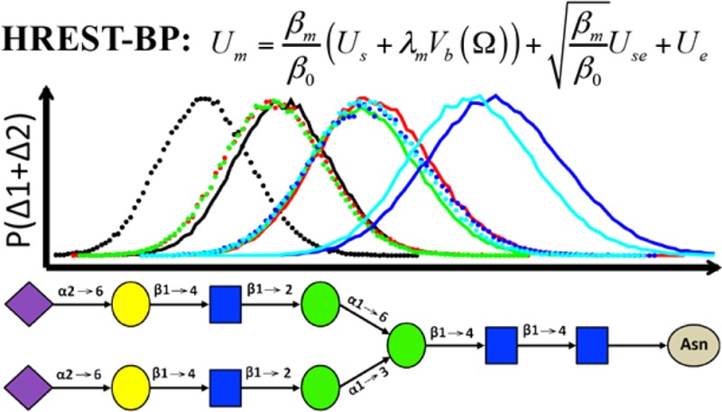
To follow the terminology in the original REST2 paper,⁴³ the new Hamiltonian replica exchange with concurrent solute scaling and biasing potential method is named HREST-BP, using “REST” as the abbreviation for replica exchange with solute scaling. In HREST-BP, the conformational space of the system R is decomposed into two subspaces represented by the central subsystem R_s and environment R_e, which results in three interaction components of the potential energy function, the internal energy of the central subsystem U_s(R_s), the self-energy of the environment U_e(R_e), and the interaction energy between the central subsystem and environment U_se(R_s,R_e). We note that for a rigid water model, such as the TIP3P model used in the present study, U_e(R_e) is equivalent to the water–water interaction energy. In the implementation of the method, the m-th simulation replica is conducted with the following scaled and biased potential function U_m(R)

1

where V_b(Ω(R_s)) is the biasing potential applied to a set of collective variables, Ω(R_s), in the central subsystem, and λ_m is the scaling factor for the biasing potential with positive values for nonground-state (or excited-state) replicas. β₀ is the inverse temperature (β₀ = 1/k_BT₀) at which the simulation is going to be performed, and β_m is the inverse temperature (β_m = 1/k_BT_m) used to scale the potential energy of the central subsystem and interaction energy between the two subsystems at replica m. The biasing potential V_b(Ω(R_s)) is used to reduce the intrinsic potential energy barriers along the respective collective variables. It is usually constructed as the negative of an approximated free energy map along the collective variables Ω(R_s) and thus always has a negative value in the simulations.⁷ At the ground-state replica where β_m = β₀ and λ_m = 0, the potential in eq 1 recovers to the unbiased potential of the system. In HREST-BP simulations all replicas are simulated at the inverse temperature β₀ and a configurational distribution proportional to exp[−β_m(U_s(R_s) + λ_mV_b(Ω(R_s))) – (β_mβ₀)^1/2U_se(R_s,R_e) – β₀U_e(R_e)] is generated for each replica m. It is obvious that an ensemble corresponding to the higher temperature is produced at β_m < β₀ (i.e. T_m > T₀), which facilitates the transitions over energy barriers in the excited-state replicas. This scaling scheme was previously adopted by a new version of replica exchange with solute tempering (REST2), which shows significantly improved sampling efficiency over the original REST implementation.^42,43 We thus employ the REST2 solute-scaling scheme to realize our HREST-BP method. However, other schemes can be straightforwardly incorporated into the HREST-BP framework.

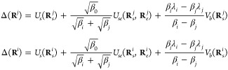
According to the Metropolis criterion, the exchange attempt between two neighboring replicas i and j (j=i+1) are accepted with the ratio

2

where Δ(Rⁱ) and Δ(R^j) are expressed as

3

Here we use the same subscript for both β and λ at a given replica, indicating that the replica exchange in β–λ space is in fact a 1D problem. This is one of the most important points in our realization of the HREST-BP method as the reduced dimensionality from 2 to 1 can greatly enhance the sampling efficiency and decrease the computational resource demands. To fully take advantage of this capability it is necessary to effectively determine the parameter distribution for both β and λ in the current 1D HREST-BP implementation. Following a similar procedure used to derive the scaling factors in H-REX with bpCMAP simulations,⁷ the equation for parameter determination can be derived under the condition of equal acceptance ratio (AR) between neighboring replicas⁵⁸⁻⁶² and the assumption of a δ-function distribution of the Δ energy term

4

where a_i and a_j are the average values of the Δ terms in neighboring replicas i and j, respectively; k and l (l=k+1) are another two neighboring replicas. The mean value of the Δ potential is composed of two terms, the temperature scaled potential term Δ₁ = U_s + (√β₀/(√β_i + √β_j))U_se and the biasing potential term Δ₂ = ((β_iλ_i – β_jλ_j)/(β_i – β_j))V_b. In order to conveniently obtain the β and λ parameters for each excited-state replica, a two-step scheme is suggested to first determine the distribution of β and then λ. For the β determination, we assume that Δ₁ has a linear dependence with respect to temperature, resulting in an exponential distribution of the temperatures

5

Use of such a temperature distribution has been shown to be reasonable in a number of replica exchange simulation studies.^{42,43,63−65} Once the temperature distribution is known, the λ factor can be determined according to the following equation

6

where V_bⁱ, V_b, V_b^k, and V_b are the average values of the biasing potential V_b(Ω(R_s)) in replicas i, j, k, and l, respectively. To get λ values from eq 6, trial simulations are required to get the λ dependence of V_b at each temperature. In the above equations, the values of const, const1, and const2 are used to tune the acceptance ratio in the parameter determination procedure.

From the definition of the scaled and biased potential in eq 1, HREST-BP recovers to H-REX when β_m is set to β₀ for all replicas. On the other hand, if λ_m = 0 or V_b(Ω(R_s)) = 0 for all replicas, the REST2 Hamiltonian is recovered from the HREST-BP. Therefore, HREST-BP is a combination of the Hamiltonian solute scaling of the central subsystem in REST2 and Hamiltonian biasing along a number of targeted collective variables in H-REX. With increasing size of the central subsystem, the sampling enhancement of REST2 is dispersed into all available solute DOFs and is thus inefficient in high energy barrier transitions that usually only exist in a small number of collective DOFs. In contrast to REST2, H-REX can specifically enhance the sampling within a set of predefined DOFs by the addition of biasing potentials along them. However, the DOFs other than the targeted ones included into the biasing potentials are not significantly enhanced in H-REX, which leads to insufficient sampling along those variables with hidden barriers. By combining REST2 and H-REX, HREST-BP can specifically enhance the sampling about the targeted collective variables, which usually have higher energy barriers, and simultaneously improve the sampling in the remaining DOFs that may possess lower hidden barriers. This combination is important for the conformational sampling of complex carbohydrates, which have coupled localized motions along the sugar glycosidic linkages that have high-energy barriers and the long-distance motions between different fragments that have low-energy barriers that are hard to identify a priori.

As discussed above, the biasing potential V_b(Ω(R_s)) is constructed as the negative of an approximated free energy map and has a negative value in the simulations.⁷ The contribution of this term to the Metropolis acceptance ratio can be written as

7

The biasing potential samples a more negative value at higher replicas, and thus the term (V_b(Ω(R_s^j)) – V_b(Ω(R_s))) is a negative value for most of the sampled conformations. Thus, whether Δ_Vb is positive or negative depends on the sign of (β_iλ_i – β_jλ_j) (i.e. (λ_iT_j – λ_jT_i)/k_BT_iT_j), which is typically negative as λ_j/λ_i ≥ T_j/T_i for most simulation systems. The condition λ_j/λ_i ≥ T_j/T_i reflects the fact that perturbations of specific DOFs (λ_i) would allow larger replica intervals than those on all DOFs (T_i). Therefore, Δ_Vb is typically negative, which would lead to smaller acceptance ratios in HREST-BP compared to standalone REST2 or H-REX, a cost we assume needs to be paid when reformulating REST2 and H-REX into the 1D HREST-BP method. However, the energy barrier in HREST-BP is reduced simultaneously from the addition of both the biasing potentials and the Hamiltonian solute scaling, whereas only one of the two factors contributes to the barrier reduction in either standalone REST2 or H-REX. Thus, the temperature and λ can be smaller in the highest excited-state replica of HREST-BP in comparison to either standalone REST2 or H-REX to achieve the same amount of biasing. Taken together, although the acceptance ratio is expected to be reduced between the neighboring replicas in HREST-BP, the number of replicas required may be comparable to or even less than that of REST2 or H-REX alone and significantly less than 2D replica exchange schemes due to the larger decrease in the energy barriers and the dimensionality reduction in the current 1D HREST-BP implementation.

Computational Details

The sampling performance of the HREST-BP method was examined with two polysaccharides that are covalently linked to the Asn dipeptide (Figure 1 a and b). We follow the terminology in ref (57) to name the two molecules, SCT and M5, which include 11 and 7 monosaccharide units, respectively, connected via different 1→2, 1→3, 1→4, 1→6, and 2→6 glycosidic linkages. These two N-glycans are found on the HIV gp120 protein or engineered antigenic glycopeptides and contribute to the epitopes of selected HIV-neutralizing antibodies.^56,57 The initial SCT model was built from the combination of two crystal structures (PDB ID 4DQO(66) and 4FQC(67)), and the Glycan Reader module in CHARMM-GUI^68,69 was used to generate the M5 model on the basis of the crystal structure 4NCO.⁵⁶ Each molecule was solvated in a cubic TIP3P water box with a dimension of 56 Å × 56 Å × 56 Å for SCT and 52 Å × 52 Å × 52 Å for M5.⁷⁰ Besides the two N-glycans, two disaccharides with 1→6 and 1→4 linkages were also constructed in a water box of 36 Å × 36 Å × 36 Å to validate our implementation (Figure 1 c and d).

Figure 1.

Saccharides used in this study: (a) N-glycan SCT, (b) N-glycan M5, (c) disaccharide with 1→6 linkage, and (d) disaccharide with 1→4 linkage. The 2D bpCMAPs were applied to the contiguous linkage dihedrals marked in blue, and 1D biasing potentials were applied to individual dihedrals marked in purple using the Woods-Saxon-type function as fitting basis. The dihedral definitions are φ(O₅^′–C₁^′–O_n–C_n)/ψ(C₁^′–O_n–C_n–C_n+1) for 1→n (n = 2, 3, or 4) linkages, φ(O₅^′–C₁^′–O₆–C₆)/ψ(C₁^′–O₆–C₆–C₅)/ω(O₆–C₆–C₅–O₅) for 1→6 linkages, χ1(N–CA–CB–CG)/χ2(CA–CB–CG–ND2), ψ_s(CB–CG–ND2–C1)/φ_s(CG–ND2–C1–O5), and the exocyclic rotation ω(O₆–C₆–C₅–O₅).

Modeling and simulations were performed with the program CHARMM with the CHARMM36 additive force field for proteins^71,72 and carbohydrates^17,19,22 and the TIP3P water model.⁷⁰ For the evaluation of energy and forces, the nonbonded terms were computed within a cutoff of 12 Å, with a smoothing switch function over the range from 10 to 12 Å used for the Lennard-Jones interactions. The long-range electrostatic interactions beyond 12 Å were treated by the particle mesh Ewald method with a charge grid of 1 Å and the 6-th order spline function for mesh interpolation.⁷³ For the charged SCT system, no counterions were added with the net charge corrected using the tinfoil boundary condition included in the Ewald implementation in CHARMM.⁷⁴ During the preparation stage, each solvated system was initially heated from 100 to 298 K under the constant volume and energy (NVE) ensemble (100 ps) and then equilibrated with 100 ps constant volume and temperature (NVT) followed by 100 ps constant pressure and temperature (NPT) MD simulations at 298 K and 1 atm. In all simulations under the NVT or NPT ensembles, including the subsequent HREST-BP, H-REX, and REST2 simulations, the temperature was maintained at 298 K using the Hoover algorithm with a thermal piston mass of 1000 kcal/mol·ps².⁷⁵ A constant pressure of 1 atm was realized using the Langevin piston algorithm with a collision frequency of 20 ps^–1 and mass of 1630 amu.⁷⁶ The covalent bonds involving hydrogen atoms were constrained with the SHAKE algorithm, and a time step of 2 fs was used.⁷⁷

In HREST-BP simulations, the solute disaccharide or N-glycan was defined as the central subsystem and solvent as the environment. Both 1D and 2D biasing potentials were adopted in each system along the dihedrals marked in Figure 1. The 2D biasing potential was constructed as the minus of an approximated free energy map within the framework of the 2D grid-based correction map (bpCMAP).^78,79 For bpCMAP construction, the approximate free energy change was derived from the 2D umbrella sampling of the gas-phase disaccharides for every sugar linkage and the D-GlcpNAc-β-1→Asn dipeptide for the side chain motion about χ1 and χ2, respectively. We have previously shown that this approach for bpCMAP construction is efficient and effective in conformational sampling of oligosaccharides.⁷ For the 1D biasing potentials along individual dihedrals, the Woods-Saxon-type function or its linear combination was used to fit the free energy profile from a high-temperature (500 K) gas-phase Langevin dynamics simulation of the M5 molecule with a total length of 2 μs. The biasing potentials were constructed using the minus of the fitted coefficient F in eq 8

8

where F, P₂, and P₁ are fitted parameters, and Ω_ref is the local minima of the free energy change about Ω. |Ω–Ω_ref | represents the absolute value of Ω–Ω_ref.

In replica exchange simulations, the temperatures or Hamiltonian scaling factors of each replica should be chosen so the acceptance ratios are similar across replicas. In practice their values are usually determined by trial and error. In HREST-BP simulations, the two scaling factors (λ and β) may be determined a priori as described above. More specifically, we assume a linear dependence of the average scaled potential Δ₁ with respect to the temperature, which results in an exponential distribution of the temperatures as expressed in eq 5. We thus set const1 = (T_N–1/T₀)^1/(N−1) in eq 5 to obtain the temperature distribution, with N being the number of replicas used. After determination of the temperatures, the λ parameter can be derived from the following protocol. (1) Performing trial HREST-BP simulation at each inverse temperature β_i (β_i ≠ β₀): 4 replicas were used with initially assigned λ values, and the exchange was realized in those 4 replicas with different λ values at the same β_i. The range of initial λ values should cover or be close to the λ_i value associated with the corresponding β_i in the production run. Each trial replica was simulated for 2 ns under the same thermodynamic ensemble as the production runs. (2) Fitting a function to the average biasing potential against λ using the data from trial simulations: the average biasing potential, {a_t}_i with t = 0, 1, 2, and 3, at each inverse temperature β_i was computed from the trial simulations and fitted as a function of λ using a polynomial basis to obtain the a_i(λ) function. (3) Substituting the fitted a_i(λ) function into eq 6 to compute the optimized λ parameter: with β₀, β₁, const2, and λ₀ = 0, the known average V_b at replica 0 (λ₀ = 0 and T₀ = 298 K), and the fitted a₁(λ), λ₁ can be calculated; then using the resulting λ₁, the average V_b value at β₁ and λ₁, β₂, and the fitted a₂(λ) to compute λ₂, and so forth. The initial const2 value can be chosen according to eq 6, for example, using λ₁ = 0.1, const2 ≈ {a₀(0)–a₁(0.1)}*0.1/0.6. Then the const2 value is adjusted to regulate the number of replicas and highest λ value for the HREST-BP simulation. For example, a smaller const2 value represents more overlap of the biasing potential distribution, and thus more replicas are needed within a given λ range. To facilitate performing the above protocol, which involves the posterior computation of average values of biasing potentials for each replica and fitting of the a_i(λ) function, a collection of 3 MatLab (MathWorks) scripts to perform these operations have been developed. These scripts are available upon request from the authors. Alternatively, the reader can use the trial and error scheme by using a linear distribution of λ as the initial guess as a near linear distribution of the λ values in the HREST-BP simulation of SCT, M5, and the 1→6 linked disaccharide was obtained.

Besides the HREST-BP, we also performed H-REX and REST2 simulations by setting β_m = 0 or λ _m = 0 in eq 1, respectively. HREST-BP was performed with the REPDSTR, BLOCK, MMFP, and CMAP modules in the CHARMM package.^80,81 The REST2 simulations were carried out with the REPDSTR and BLOCK modules. H-REX was performed using the MMFP and CMAP modules in CHARMM to add the 1D and 2D biasing potentials, respectively. Exchange attempts were performed every 2000 MD steps and accepted according to eq 2. The SCT production runs, including HREST-BP, REST2, and H-REX, were performed under the NVT ensemble at 298 K with a length of 100 ns for each replica (Table 1). The other systems, including M5 (Table S1, Supporting Information), the D-Manp-α-(1→6)-D-Manp-β-1-OMe disaccharide (Table S2, Supporting Information), and the D-Glcp-β-(1→4)-D-Glcp-β-1-OMe disaccharide (Table S3, Supporting Information), were simulated under the NPT ensemble at 1 atm and 298 K with 20 ns for each replica, with the HREST-BP simulation of M5 extended to 90 ns to check the convergence.

Table 1. Parameter Distribution and Acceptance Ratios (AR) in the SCT Simulation System.

replica index	T (K)	λ	AR/HREST-BPb (%)	AR/REST2 (%)	AR/H-REXb (%)
0	298	0.00	22.8	27.2	65.5
1	316	0.10	20.8	27.0	55.9
2	335	0.23	20.5	27.4	54.6
3	356	0.32	19.0	28.0	51.2
4	377	0.43	18.3	28.2	47.7
5	400	0.50	20.9	28.3	55.6
AARa			20.4	27.7	55.1

^aAAR – the average acceptance ratio over all 6 replicas in each simulation.

^bThe biasing potentials used are marked in Figure 1a.

In the present study the scaling of the solute potential in HREST-BP or REST2 methods included scaling of all the intramolecular energy terms, including nonbonded interactions, within the solute according to the effective temperature. In the original REST2 implementation only the dihedral and nonbonded interactions were scaled, with the bond and angle terms not included in the scaling.⁴³ Accordingly, we examined the influence of the two schemes with the 1→6 linked disaccharide model with a simulation time of 20 ns for each replica and found a larger acceptance ratio if the original REST2 scaling is used (46.4% vs 34.8% for REST2 and 39.1% vs 29.2% for HREST-BP). The similar change in the acceptance ratio in HREST-BP and REST2 is expected from eq 3 since the term governing acceptance ratio in REST2 is the main factor in determining the HREST-BP exchange. Future studies will investigate the sampling performance with different scaling schemes beyond the two approaches mentioned above.

Data Analysis

From the simulations, the potential of mean force (PMF) or free energy change along a collective variable Ω was computed from the conformational distribution ρ(R) in the ground-state replica under the NVT ensemble as

9

where N_s is the number of snapshots recorded in the trajectory and Δ(Ω(R_j) – ω_i) = 1 if Ω(R_j) is within the bin [w_i – Δw/2,w_i + Δw/2] and otherwise Δ(Ω(R_j) – ω_i) = 0. The same expression as eq 9 is used for the Gibbs free energy change under the NPT ensemble. The convergence of the PMFs was characterized by the root-mean-square deviation of the PMF (pRMSD) computed at a given simulation time t relative to the reference profiles

10

where N₁ and N₂ are the number of collective variables and sampled bins in the PMF calculation of individual collective variables at time t, respectively; A_ki and A_ki^ref are the free energies for k-th variable at i-th bin, and A_ki is the reference PMF computed using the entire ground-state trajectory. This quantity indicates how fast the simulation converges along these variables.

To measure the biasing compensation in the context of the ability of the biasing potentials to flatten the free energy surface, the configurational entropy associated with a given set of collective variables was estimated as^55,82

11

with M being the number of collective variables along which the entropy is computed. Since the entropy is maximized at a uniform distribution of each ρ(ω_m), which corresponds to a complete compensation of the free energy landscape, a larger value of entropy represents more effective biasing compensation on these collective variables. Two types of configurational entropy were examined, one for localized motions along the linkage dihedrals and the other for 3D spatial distribution of several representative monosaccharides in SCT. The 3D probability distribution maps of the individual monosaccharides were constructed for the SCT system using the Asn dipeptide as the alignment reference.⁸³⁻⁸⁵ A 100 Å × 100 Å × 100 Å cubic grid was built to encompass the Asn dipeptide with a grid spacing of 3 Å, which is approximately the distance between the diagonal atoms in the sugar ring. The probability distribution of each monosaccharide unit was represented as the occupied number of frames in the trajectory for every grid point normalized such that the grid point with largest occupancy has a value of 1. As the snapshots were aligned with respect to the Asn dipeptide the distributions represent the relative orientation of the sugar units with respect to the peptide that would, for example, be present in a rigid protein.

Results and Discussions

The HREST-BP simulation was carried out in CHARMM using the replica exchange module REPDST with BLOCK to scale the solute–solute and solute–solvent interactions, with CMAP and MMFP to apply the 2D and 1D biasing potentials, respectively. To validate the correctness of this implementation, two solvated disaccharides with 1→4 and 1→6 linkages were simulated using HREST-BP, H-REX, and REST2 with different biasing potentials and parameter distributions (Figure 1c-d and Tables S2 and S3 in the Supporting Information). The assumption related to this examination is that the free energy landscape from the ground-state replica should be independent of the simulation setup, which suggests that the same ensemble is sampled. To this end, the PMF profiles from H-REX simulations were used as reference since that method has been validated in previous simulations.^7,9,13 As shown in Figure 2, all simulations give the same free energy changes about the dihedrals that define the conformational propensity of the disaccharides. This indicates correctness of the scaling and biasing implementations in the HREST-BP simulation. It is noted that the HREST-BP method does not have an obvious advantage over H-REX or REST2 for the disaccharide simulations since there is no long-distance interaction in these small systems that are not effectively biased.

Figure 2.

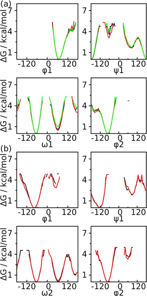
Examination of the PMF profiles for the disaccharides from different simulation methods. (a) 1→6 linked disaccharide from HREST-BP (black), H-REX (green), and REST2 (red) and (b) 1→4 linked disaccharide from two different HREST-BP simulations with one using only the 2D bpCMAP along the linkage dihedrals φ1/ψ1 (black) and the other using both the 2D bpCMAP along the linkage dihedrals and 1D biasing potential about the individual dihedrals ω2, ω3, and φ2 (red).

The development of HREST-BP aims to improve sampling in simulations of complex molecular systems in explicit solvent environments. To this end, two N-glycan molecules were employed to examine the sampling efficiency of the method; SCT includes 11 monosaccharide units and M5 includes 7 monosaccharides (Figure 1a-b). Different simulation setups were used for the two systems to identify suitable parameters for N-glycan simulations in HREST-BP. For SCT, a total of 6 replicas were used with temperature and λ ranges of [298 K, 400 K] and [0, 0.50], respectively (Table 1). Ten replicas were adopted for M5 since more 1D biasing potentials were applied in this system (Figure 1b), and the temperature and λ ranges were [298 K, 600 K] and [0, 0.64], respectively (Table S1, Supporting Information). Because the main goal of this study is to examine the usefulness of HREST-BP, we focus on the more complicated SCT system to illustrate the utility of the method and present the M5 results in the Supporting Information.

To examine the effectiveness of the temperature and λ parameters from our estimation protocol, we analyzed the dependence of the average scaled potential Δ₁ = U_s + (√β₀/(√β_i + √β_j))U_se with respect to the scaling temperature. This relationship was well fitted to a linear function (Figure 3a), suggesting that the exponential (or geometric) distribution of temperature is a good choice for N-glycan molecules solvated with the TIP3P water model in the HREST-BP simulations. Under this temperature assignment, the probability distribution of the temperature scaled potential Δ₁ shows sufficient overlap between the neighboring replicas, which is one of the two terms that determine the acceptance ratio (Figure 3b). In addition to Δ₁ the other term affecting the exchange acceptance is related to the biasing potential V_b in Δ₂ = ((β_iλ_i −β_jλ_j)/(β_i – β_j))V_b. As discussed in the methods section, the addition of V_b in HREST-BP would reduce the acceptance ratio as more negative V_b values were sampled at higher replicas (Figure 3c). However, we would expect a small reduction in the acceptance ratio due to the relatively small values of V_b in comparison to Δ₁ if a proper estimation scheme is used. As the term Δ₁ is the sole factor controlling the exchange in REST2 (λ = 0), this reduction is illustrated in Table 1 by comparing the acceptance ratio between HREST-BP and REST2 simulations (Tables S1–S3, Supporting Information for the other systems). However, while the acceptance ratios are smaller, the probability distribution of the two acceptance determinants, Δ = Δ₁ + Δ₂, shows good overlap for

and

sampled in neighboring replicas i and j (j=i+1) that determines the acceptance ratio in HREST-BP simulations (Figure 3d). Figure 4 shows the random walk of replicas in the HREST-BP simulation; an average of 29 round trips was observed within a simulation time of 100 ns for each replica. These results indicate efficient visits in parameter space and validate the effectiveness of our parameter estimation protocol in the HREST-BP simulations for N-glycans.

Figure 3.

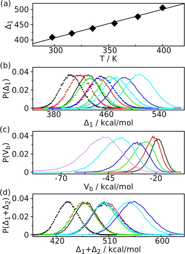
Potential energy distribution in HREST-BP simulation of SCT. (a) Linear fit of average scaled potential Δ₁ = U_s + (√β₀/(√β_i + √β_j))U_se (in kcal/mol) versus the scaling temperature used in each replica. (b) The overlap of the probability distributions of the scaled potential Δ₁ = U_s + (√β₀/(√β_i + √β_j))U_se for each pair of neighboring replicas i (dotted line) and j (j=i+1) (solid line). It is the overlap of probability distributions of Δ₁ = U_s(Rⁱ) + (√β₀/(√β_i + √β_j))U_se(Rⁱ) and Δ₁ = U_s(R^j) + (√β₀/(√β_i + √β_j))U_se(R^j) that determines the acceptance ratio between replicas i and i+1. The probability distribution overlap is plotted in different colors for each pair of neighboring replicas, black for replicas 0 and 1, red for 1 and 2, green for 2 and 3, blue for 3 and 4, and cyan for 4 and 5. (c) Probability distribution of the biasing potential V_b in replicas 0 (black), 1 (red), 2 (green), 3 (blue), 4 (cyan), and 5 (purple). (d) The overlap of the probability distributions of the scaled and biased potential Δ = U_s + (√β₀/(√β_i + √β_j))U_se + ((β_iλ_i −β_jλ_j)/(β_i – β_j))V_b for each pair of neighboring replicas i (dotted line) and j (j=i+1) (solid line). The same color scheme is used as in panel (b).

Figure 4.

Random walk of 3 representative replicas 1 (top), 3 (middle), and 5 (bottom) in the HREST-BP simulation of SCT.

The conformational changes in SCT include both the localized motions around the glycosidic linkages and long-distance motions between remote monosaccharides in different branches of the polysaccharides. The two types of change are coupled, i.e. a certain linkage conformation will favor a specific relative orientation of the branches, and vice versa. The free energy barriers associated with these degrees of freedom are higher than 6 kcal/mol for the linkage motions and <3 kcal/mol for the long-distance changes (Figures 5 and 6). In HREST-BP, the higher energy barriers are reduced simultaneously by the temperature scaling and the biasing potentials that specifically enhance the sampling around these linkages, while the lower energy barriers are overcome with the Hamiltonian scaling of the whole solute, thereby providing an overall sampling enhancement of the full range of accessible conformation of the N-glycan. By reformulating the overall temperature scaling and specific biasing potential into the 1D replica exchange, sampling is well balanced for these two types of motion. This is evident in Figure 5 showing all the PMF profiles around the sugar linkages to converge in the simulations of HREST-BP, H-REX, and REST2. For these linkage motions, all three methods give reasonably good sampling around the statistically important low-free energy states on a simulation time of 100 ns. However, detailed examination of these PMF profiles shows that HREST-BP produces an overall better sampling in comparison to H-REX and REST2. For example, more regions are sampled in HREST-BP than REST2 around the dihedrals φ1, ω1, and φ3, whereas only one dihedral φ2′ is sampled better in REST2. Compared to H-REX, HREST-BP has better sampling along dihedrals φ1, ψ1, ω1, and φ2 (Figure 5). The sampling performance was further examined using 20 ns of simulation time with the results from 100 ns trajectory as reference. In 20 ns HREST-BP shows more sampling about the linkage dihedrals φ1, ψ1, ω1, φ2, φ3, ψ3, φ3′, ψ5′, φ6, and ψ6 than REST2 and φ1, ω1, φ2, and φ3 than H-REX (Figure S1, Supporting Information). These results suggest that the concurrent enhancement from biasing potentials and Hamiltonian scaling in HREST-BP produces better sampling around DOFs with high-energy barriers, while the relative inefficiency of REST2 along several dihedrals arises from the dispersion of sampling enhancement into all DOFs of the solute.

Figure 5.

Free energy profiles along the linkage dihedrals of SCT in the simulation with HREST-BP (black), H-REX (green), and REST2 (red). The total 100 ns of ground-state trajectory was used for PMF calculation.

Figure 6.

Free energy profiles along the distance between the center of mass (DCOM) of different sugar rings of SCT in the simulation with HREST-BP (black), H-REX (green), and REST2 (red). The total 100 ns (bold line) and first 50 ns (thin line) of ground-state trajectory were used for the PMF calculation. The DCOM profiles with more than one local minima were shown in this figure.

The long-distance motions were analyzed as PMF profiles along the distances between centers of mass (DCOM) of noncontiguous monosaccharides (Figure 6). Both HREST-BP and REST2 simulations approximately converge to similar surfaces within a simulation time of 50 ns. It is interesting that some PMF profiles from H-REX do not converge to the same surfaces even within a 100 ns simulation. The same problem is also observed in the smaller M5 system (Figure S2, Supporting Information). These results suggest the H-REX simulation with only localized biasing potentials around the linkages converge much more slowly with respect to the sampling of long-distance motions. This emphasizes the importance of the inclusion of the overall enhanced sampling with Hamiltonian temperature scaling in the N-glycan simulations. Thus, while all three methods can sample the linkage motions with a similar level of convergence only HREST-BP and REST2 give correct sampling of the long-distance motions within the simulation length performed in this study.

From the results in Figure 5 and 6, a temperature range from 298 to 400 K is a reasonably good choice in HREST-BP simulation to balance the conformational sampling of localized linkage motions and long-distance changes. The larger temperature range used in the M5 system is not necessary for glycan systems with HREST-BP (Table S1, Supporting Information). Furthermore, the presence or absence of 1D biasing potentials acting on the exocyclic hydroxyl or N-acetyl groups does not produce obvious differences in the free energy landscape of M5 with HREST-BP (data not shown). This indicates that the use of high temperature (600 K for the highest replica in M5) in HREST-BP can efficiently overcome the energy barriers associated with these DOFs.

To understand the sampling performance in more detail, we examined the exploration rate and convergence rate of HREST-BP of the SCT system. To compute the local exploration rate, the conformational space is defined according to the linkage conformations. Each linkage dihedral was divided into three bins, [0°, 120°], [−120°, 0°], and [−180°, −120°] and [120°, 180°], corresponding to different local minima as observed in the PMFs shown in Figure 5. The exploration rate is calculated as the sum of the total number of visited conformations as a function of simulation time. The result in Figure S3 shows a comparable exploration rate for the three methods during the first 40 ns. It suggests the three methods visit the local minima accessible to the glycosidic linkages with almost the same rate as the linkage motions are well converged within a simulation time of 20 ns (Figure S1, Supporting Information).

The convergence rate was also measured for both the local glycosidic linkages and long-distance motions using the PMF RMSD (pRMSD) metric for the different variables as defined in eq 10. The result in Figure 7a shows faster convergence in HREST-BP and H-REX than REST2 for the localized linkage motions. For the long-distance motions, HREST-BP gives the fastest convergence as shown in Figure 7b. It is noted that these convergence rates are measured with respect to the PMF from the 100 ns trajectory at the end of each simulation with the different methods. Taken together, the HREST-BP has a faster convergence rate in sampling both linkage and long-distance motions than REST2 and a similar convergence rate with H-REX about the localized linkage motions.

Figure 7.

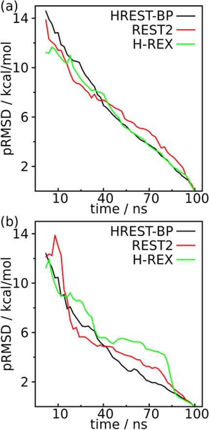
Convergence rate of different simulations as represented by PMF RMSD (pRMSD) for (a) the marked linkage dihedrals in the structural model of SCT with more than one local minima and (b) the distances of centers of mass (DCOM) between different sugar rings of SCT as shown in Figure 6.

An additional measure of the ability of the REX methods to improve sampling is the energetic “flatness” of the biased system, as quantified by the configurational entropy associated with a given set of collective variables (eq 11). The entropy value represents the extent to which the original free energy landscape is compensated in each replica. The entropy value along the localized dihedrals in Figure 8a clearly indicates that the most effective biasing is the HREST-BP method. This is expected as HREST-BP benefits simultaneously from the Hamiltonian scaling of the whole solute and solute–solvent interactions and potential biasing along these specific dihedrals. Moreover, it shows that the biasing potentials in H-REX are more effective than the Hamiltonian scaling in REST2 along these localized linkage motions. The biasing of long-distance motions was represented using the entropy values from 3D spatial distributions of several representative monosaccharides in different sugar fragments (Figure 8b-f). Only HREST-BP and REST2 include direct long-distance bias in the simulations, leading to an increasing entropy value in the higher replicas. Although no direct long-distance bias is present in H-REX, the large entropy values suggest the sampling of the linkages is coupled to the long-distance conformational changes. However, it is noted that the lack of long-distance biasing potentials in H-REX makes the convergence rate much slower in sampling of these conformational changes (Figure 6 and Figure S2 in the Supporting Information). In summary, the same amount of biasing can be achieved in HREST-BP with a smaller number of replicas because of the concurrent effect of the two Hamiltonian biasing terms as compared to H-REX or REST2 for which only one type of biasing is used.

Figure 8.

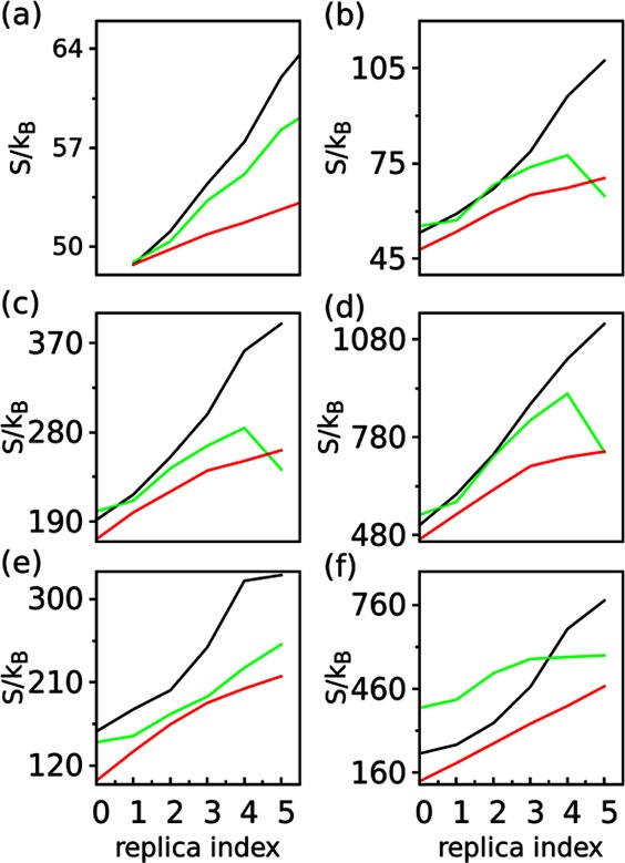
Configurational entropy used to measure the biasing compensation about the given collective variables for the replicas in the HREST-BP (black), H-REX (green), and REST2 (red) simulations. (a) Entropy along all the marked dihedrals in Figure 1. (b-f) Entropy for the 3D spatial distribution of monosaccharides (b) 3, (c) 5, (d) 7, (e) 9, and (f) 11.

The relative orientation of an N-glycan with respect to the peptide to which it is connected is critical, for example, to the molecular recognition between N-glycan antigens and antibodies. To provide more insights on this issue, the spatial distribution sampled by individual sugar units in SCT was analyzed. Three rigid fragments were identified based on small intramolecular RMSD fluctuations (Figure S4, Supporting Information), including -D-Manp(3)-β-(1→4)-D-GlcpNAc(2)-β-(1→4)-D-GlcpNAc(1)-β-1-, -D-Galp(6)-β-(1→4)-D-GlcpNAc(5)-β-(1→2)-D-Manp(4)-α-1-, and -D-Galp(10)-β-(1→4)-D-GlcpNAc(9)-β-(1→2)-D-Manp(8)-α-1-. These fragments are connected to each other through flexible 1→6 and 2→6 linkages, in addition to the χ1/ χ2 and ψ_s/φ_s dihedrals linking the glycan to the Asn dipeptide. To evaluate the sampling about these flexible dihedrals, the simulated free energy maps were compared to dihedral distributions from crystal structures that include the respective linkages.⁸⁶ Figure 9 shows that the HREST-BP simulation of SCT samples the majority of the conformational states observed in the crystal structures about these flexible linkages, although some regions are not being sampled.

Figure 9.

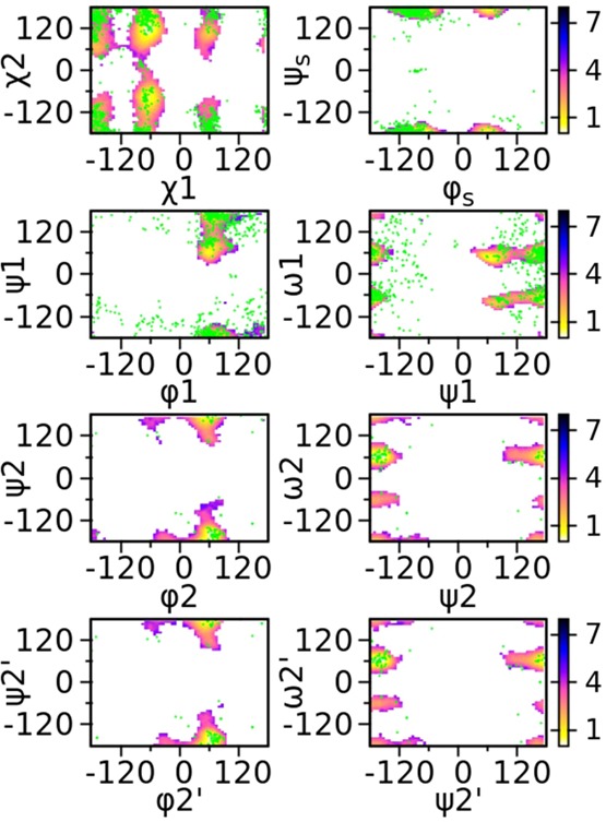
Comparison between sampled free energy landscape (contour surfaces, in kcal/mol) and conformational distributions from crystal structures (in dot) for the 1→6, 2→6, χ1/χ2, and φ_s/ψ_s linkages in SCT. The free energy map was computed from the ground-state replica of HREST-BP simulation.

To identify why some conformations are not sampled along these flexible linkages, the free energy maps along the same dihedrals were computed in model compounds (Figure S5, Supporting Information). The results show a good correspondence between simulated local minima in the PMF 2D maps and the crystal conformations. This suggests that the current force field accurately describes the energetics of these flexible linkages. Crystal conformations present in the high-free energy regions of SCT PMFs (Figure 9) are thus either stabilized by interactions with the environment, such as proteins, in the crystals or cannot be sampled in the larger N-glycan, versus the di- and trisaccharides that are predominate in the crystal survey, due to steric clashes between the noncontiguous monosaccharides in SCT.

Conclusions

The presented 1D HREST-BP method can significantly reduce the computational cost in comparison to multidimensional extensions of REX. It combines the advantages of overall enhanced sampling from REST2 and specific enhancement of selected collective variables using biasing potentials in H-REX. This complementarity is especially important for systems with hierarchical motions that are controlled by different energy barriers, in which Hamiltonian scaling is applied to the whole solute subsystem to enhance the sampling of long-distance motions, and simultaneously biasing potentials are added to accelerate the barrier transitions about the targeted collective variables that typically have higher energy barriers. Because of its implementation in a 1D fashion and Hamiltonian scaling is applied to the entire subsystem of interest, the number of replicas can be small, similar to that commonly used in H-REX and smaller than that used in REST2 simulations, where higher effective temperatures are required to accelerate high-energy barrier transitions. In comparison to H-REX, the HREST-BP does not have an obvious advantage for the study of localized motions or small sized systems. However, while H-REX can minimize the required number of replicas, it converges more slowly than HREST-BP along long-distance DOFs when biasing potentials are not applied to those collective variables, which are typically difficult to identify and define in complex molecular systems. In contrast, it is much easier to define the collective variables responsible for localized DOFs from chemical intuition or prior knowledge, as exemplified by the glycosidic linkage dihedrals in carbohydrates. For these localized variables, the biasing potential can be constructed from the small gas-phase or solvated model systems (e.g., disaccharides), which has been shown to be efficient and effective for the study of complex carbohydrate conformational properties.⁷

The 1D HREST-BP scheme can be further generalized using more flexible ways to construct the biasing Hamiltonian compared to eq 1. For example, standard T-REX can be used for the “globally” enhanced sampling part in the presence or absence of explicit solvent instead of REST2, with U_m(R) = (β_m/β₀)(U_s(R_s) + U_se(R_s,R_e) + U_e(R_e) + λ_mV_b(Ω(R_s))), as the thermodynamic quantities of interest for a classical system with a potential energy E at temperature T are equivalent to those with a potential energy β_m/β₀*E at temperature T₀. The general principle is that different types of perturbation in the Hamiltonian are additive so that replica exchange can be carried out in a 1D fashion. As shown in this study, combining different (global and localized) potential biasing leads to reduced values of the acceptance ratios but is more effective in lowering energy barriers, resulting in a comparable total number of replicas to that in standalone T-REX or H-REX simulations. We anticipate the general utility of the HREST-BP simulation method in a variety of macromolecular systems, such as, proteins, RNA, and DNA, which involve coupled localized motions and long-distances changes in their functioning processes.

Glossary

ABBREVIATIONS

1D

one-dimensional

2D

two-dimensional

3D

three-dimensional

BP

biasing potential

bpCMAP

biasing potential using 2D grid-based correction map

DCOM

distance of centers of mass

DOFs

degrees of freedom

HREST-BP

Hamiltonian replica exchange with concurrent solute scaling and biasing potential

H-REX

Hamiltonian replica exchange

HT-REX

replica exchange in both Hamiltonian and temperature space

MD

molecular dynamics

MSES

multiscale enhanced sampling

NPT

thermodynamic ensemble of constant particle number, pressure, and temperature

NVE

thermodynamic ensemble of constant particle number, volume, and energy

NVT

thermodynamic ensemble of constant particle number, volume, and temperature

PME

particle mesh Ewald

PMF

potential of mean force

pRMSD

the root-mean-square deviation of PMF

RECT

replica exchange with collective variable tempering

REST

replica exchange with solute tempering

REST2

a new version of replica exchange with solute tempering

REX

replica exchange

RMSD

root-mean-square deviation

T-REX

replica exchange in temperature space

WEUSMD

window exchange umbrella sampling molecular dynamics

Supporting Information Available

The simulation parameters for M5 and two disaccharides in Tables S1–S3, the PMF profiles about linkage motions of SCT in Figure S1, the long-distance PMF profiles of M5 in Figure S2, the exploration rate of SCT in Figure S3, the RMSD variation of SCT in Figure S4, and the comparison between crystal survey of flexible dihedrals and 2D PMF map from disaccharide models in Figure S5. The Supporting Information is available free of charge on the ACS Publications website at DOI: 10.1021/acs.jctc.5b00243.

The authors declare no competing financial interest.

References

- Shukla R. K.; Tiwari A. Crit. Rev. Ther. Drug Carrier Syst. 2011, 283255–292. [DOI] [PubMed] [Google Scholar]
- Huang Y.; Wun C. Expert Rev. Vaccines 2010, 9111257–1274. [DOI] [PubMed] [Google Scholar]
- Astronomo R. D.; Burton D. R. Nat. Rev. Drug Discovery 2010, 94308–324. [DOI] [PMC free article] [PubMed] [Google Scholar]
- Essentials of Glycobiology, 2nd ed.; Cold Spring Harbor Laboratory Press: Cold Spring Harbor, NY, 2009. [PubMed] [Google Scholar]
- DeMarco M. L.; Woods R. J. Glycobiology 2008, 186426–440. [DOI] [PMC free article] [PubMed] [Google Scholar]
- Dwek R. A. Biochem. Soc. Trans. 1995, 2311–25. [DOI] [PubMed] [Google Scholar]
- Yang M.; MacKerell A. D. Jr. J. Chem. Theory Comput. 2015, 112788–799. [DOI] [PMC free article] [PubMed] [Google Scholar]
- Patel D. S.; He X.; MacKerell A. D. Jr. J. Phys. Chem. B 2015, 119, 637–652. [DOI] [PMC free article] [PubMed] [Google Scholar]
- Patel D. S.; Pendrill R.; Mallajosyula S. S.; Widmalm G.; MacKerell A. D. Jr. J. Phys. Chem. B 2014, 118112851–2871. [DOI] [PMC free article] [PubMed] [Google Scholar]
- Krishnan S.; Liu F.; Abrol R.; Hodges J.; Goddard W. A.; Prasadarao N. V. J. Biol. Chem. 2014, 2894530937–30949. [DOI] [PMC free article] [PubMed] [Google Scholar]
- Mallajosyula S. S.; Adams K. M.; Barchi J. J.; MacKerell A. D. Jr. J. Chem. Inf. Model. 2013, 5351127–1137. [DOI] [PMC free article] [PubMed] [Google Scholar]
- He X.; Hatcher E.; Eriksson L.; Widmalm G.; MacKerell A. D. Jr. J. Phys. Chem. B 2013, 117257546–7553. [DOI] [PMC free article] [PubMed] [Google Scholar]
- Mallajosyula S. S.; MacKerell A. D. Jr. J. Phys. Chem. B 2011, 1153811215–11229. [DOI] [PMC free article] [PubMed] [Google Scholar]
- Hatcher E.; Sawen E.; Widmalm G.; MacKerell A. D. Jr. J. Phys. Chem. B 2011, 1153597–608. [DOI] [PMC free article] [PubMed] [Google Scholar]
- Stanca-Kaposta E. C.; Gamblin D. P.; Cocinero E. J.; Frey J.; Kroemer R. T.; Fairbanks A. J.; Davis B. G.; Simons J. P. J. Am. Chem. Soc. 2008, 1303210691–10696. [DOI] [PubMed] [Google Scholar]
- Andre S.; Kozar T.; Schuberth R.; Unverzagt C.; Kojima S.; Gabius H.-J. Biochemistry 2007, 46236984–6995. [DOI] [PubMed] [Google Scholar]
- Guvench O.; Greene S. N.; Kamath G.; Brady J. W.; Venable R. M.; Pastor R. W.; Mackerell A. D. Jr. J. Comput. Chem. 2008, 29152543–2564. [DOI] [PMC free article] [PubMed] [Google Scholar]
- Kirschner K. N.; Yongye A. B.; Tschampel S. M.; Gonzalez-Outeirino J.; Daniels C. R.; Foley B. L.; Woods R. J. J. Comput. Chem. 2008, 294622–655. [DOI] [PMC free article] [PubMed] [Google Scholar]
- Guvench O.; Hatcher E.; Venable R. M.; Pastor R. W.; MacKerell A. D. Jr. J. Chem. Theory Comput. 2009, 592353–2370. [DOI] [PMC free article] [PubMed] [Google Scholar]
- Hatcher E.; Guvench O.; MacKerell A. D. Jr. J. Phys. Chem. B 2009, 1133712466–12476. [DOI] [PMC free article] [PubMed] [Google Scholar]
- Raman E. P.; Guvench O.; MacKerell A. D. Jr. J. Phys. Chem. B 2010, 1144012981–12994. [DOI] [PMC free article] [PubMed] [Google Scholar]
- Guvench O.; Mallajosyula S. S.; Raman E. P.; Hatcher E.; Vanommeslaeghe K.; Foster T. J.; Jamison F. W.; MacKerell A. D. Jr. J. Chem. Theory Comput. 2011, 7103162–3180. [DOI] [PMC free article] [PubMed] [Google Scholar]
- Hansen H. S.; Huenenberger P. H. J. Comput. Chem. 2011, 326998–1032. [DOI] [PubMed] [Google Scholar]
- Wood N. T.; Fadda E.; Davis R.; Grant O. C.; Martin J. C.; Woods R. J.; Travers S. A. PLoS One 2013, 811e80301. [DOI] [PMC free article] [PubMed] [Google Scholar]
- Yang M.; Yang L.; Gao Y.; Hu H. J. Chem. Phys. 2014, 1414044108. [DOI] [PubMed] [Google Scholar]
- Maragliano L.; Vanden-Eijnden E. Chem. Phys. Lett. 2006, 4261–3168–175. [Google Scholar]
- Rosso L.; Minary P.; Zhu Z. W.; Tuckerman M. E. J. Chem. Phys. 2002, 116114389–4402. [Google Scholar]
- Hu H.; Yang W. Annu. Rev. Phys. Chem. 2008, 59, 573–601. [DOI] [PMC free article] [PubMed] [Google Scholar]
- Hu Y.; Hong W.; Shi Y.; Liu H. J. Chem. Theory Comput. 2012, 8103777–3792. [DOI] [PubMed] [Google Scholar]
- Kaestner J. Wiley Interdiscip. Rev.: Comput. Mol. Sci. 2011, 16932–942. [Google Scholar]
- Chipot C.; Lelievre T. SIAM J. Appl. Math. 2011, 7151673–1695. [Google Scholar]
- Yang L.; Gao Y. Q. J. Chem. Phys. 2009, 13121214109. [DOI] [PubMed] [Google Scholar]
- Zheng L.; Chen M.; Yang W. Proc. Natl. Acad. Sci. U. S. A. 2008, 1055120227–20232. [DOI] [PMC free article] [PubMed] [Google Scholar]
- Darve E.; Rodriguez-Gomez D.; Pohorille A. J. Chem. Phys. 2008, 12814144120. [DOI] [PubMed] [Google Scholar]
- Micheletti C.; Laio A.; Parrinello M. Phys. Rev. Lett. 2004, 9217170601. [DOI] [PubMed] [Google Scholar]
- Sugita Y.; Okamoto Y. Chem. Phys. Lett. 1999, 3141–2141–151. [Google Scholar]
- Kannan S.; Zacharias M. Proteins: Struct., Funct., Bioinf. 2009, 762448–460. [DOI] [PubMed] [Google Scholar]
- Swendsen R. H.; Wang J. S. Phys. Rev. Lett. 1986, 57212607–2609. [DOI] [PubMed] [Google Scholar]
- Fukunishi H.; Watanabe O.; Takada S. J. Chem. Phys. 2002, 116209058–9067. [Google Scholar]
- Nishima W.; Miyashita N.; Yamaguchi Y.; Sugita Y.; Re S. J. Phys. Chem. B 2012, 116298504–8512. [DOI] [PubMed] [Google Scholar]
- Re S.; Miyashita N.; Yamaguchi Y.; Sugita Y. Biophys. J. 2011, 10110L44–L46. [DOI] [PMC free article] [PubMed] [Google Scholar]
- Liu P.; Kim B.; Friesner R. A.; Berne B. J. Proc. Natl. Acad. Sci. U. S. A. 2005, 1023913749–13754. [DOI] [PMC free article] [PubMed] [Google Scholar]
- Wang L.; Friesner R. A.; Berne B. J. J. Phys. Chem. B 2011, 115309431–9438. [DOI] [PMC free article] [PubMed] [Google Scholar]
- Shim J.; Zhu X.; Best R. B.; MacKerell A. D. Jr. J. Comput. Chem. 2013, 347593–603. [DOI] [PMC free article] [PubMed] [Google Scholar]
- Moradi M.; Tajkhorshid E. J. Chem. Theory Comput. 2014, 1072866–2880. [DOI] [PMC free article] [PubMed] [Google Scholar]
- Bolhuis P. G.; Dellago C.; Chandler D. Proc. Natl. Acad. Sci. U. S. A. 2000, 97115877–5882. [DOI] [PMC free article] [PubMed] [Google Scholar]
- Meng Y.; Roitberg A. E. J. Chem. Theory Comput. 2010, 641401–1412. [DOI] [PMC free article] [PubMed] [Google Scholar]
- Bergonzo C.; Henriksen N. M.; Roe D. R.; Swails J. M.; Roitberg A. E.; Cheatham T. E. J. Chem. Theory Comput. 2013, 101492–499. [DOI] [PMC free article] [PubMed] [Google Scholar]
- Moradi M.; Babin V.; Roland C.; Sagui C. PLoS Comput. Biol. 2012, 84e1002501. [DOI] [PMC free article] [PubMed] [Google Scholar]
- Sugita Y.; Kitao A.; Okamoto Y. J. Chem. Phys. 2000, 113156042–6051. [Google Scholar]
- Kokubo H.; Tanaka T.; Okamoto Y. J. Comput. Chem. 2013, 34302601–2614. [DOI] [PubMed] [Google Scholar]
- Park S.; Im W. J. Chem. Theory Comput. 2012, 9113–17. [DOI] [PMC free article] [PubMed] [Google Scholar]
- Laghaei R.; Mousseau N.; Wei G. J. Phys. Chem. B 2010, 114207071–7077. [DOI] [PubMed] [Google Scholar]
- Zhang W.; Chen J. J. Chem. Theory Comput. 2014, 103918–923. [DOI] [PubMed] [Google Scholar]
- Gil-Ley A.; Bussi G. J. Chem. Theory Comput. 2015, 11, 1077–1085. [DOI] [PMC free article] [PubMed] [Google Scholar]
- Julien J.-P.; Cupo A.; Sok D.; Stanfield R. L.; Lyumkis D.; Deller M. C.; Klasse P.-J.; Burton D. R.; Sanders R. W.; Moore J. P.; Ward A. B.; Wilson I. A. Science 2013, 34261651477–1483. [DOI] [PMC free article] [PubMed] [Google Scholar]
- Amin M. N.; McLellan J. S.; Huang W.; Orwenyo J.; Burton D. R.; Koff W. C.; Kwong P. D.; Wang L.-X. Nat. Chem. Biol. 2013, 98521–526. [DOI] [PMC free article] [PubMed] [Google Scholar]
- Earl D. J.; Deem M. W. J. Phys. Chem. B 2004, 108216844–6849. [Google Scholar]
- Kone A.; Kofke D. A. J. Chem. Phys. 2005, 12220206101. [DOI] [PubMed] [Google Scholar]
- Rathore N.; Chopra M.; de Pablo J. J. J. Chem. Phys. 2005, 1222024111. [DOI] [PubMed] [Google Scholar]
- Denschlag R.; Lingenheil M.; Tavan P. Chem. Phys. Lett. 2009, 4731–3193–195. [Google Scholar]
- Prakash M. K.; Barducci A.; Parrinello M. J. Chem. Theory Comput. 2011, 772025–2027. [DOI] [PubMed] [Google Scholar]
- Huang X.; Hagen M.; Kim B.; Friesner R. A.; Zhou R.; Berne B. J. J. Phys. Chem. B 2007, 111195405–5410. [DOI] [PMC free article] [PubMed] [Google Scholar]
- Nadler W.; Hansmann U. H. E. J. Phys. Chem. B 2008, 1123410386–10387. [DOI] [PubMed] [Google Scholar]
- Nadler W.; Hansmann U. H. E. Phys. Rev. E 2007, 752026109. [DOI] [PubMed] [Google Scholar]
- Pancera M.; Shahzad-ul-Hussan S.; Doria-Rose N. A.; McLellan J. S.; Bailer R. T.; Dai K.; Loesgen S.; Louder M. K.; Staupe R. P.; Yang Y.; Zhang B.; Parks R.; Eudailey J.; Lloyd K. E.; Blinn J.; Alam S. M.; Haynes B. F.; Amin M. N.; Wang L.-X.; Burton D. R.; Koff W. C.; Nabel G. J.; Mascola J. R.; Bewley C. A.; Kwong P. D. Nat. Struct. Mol. Biol. 2013, 207804–813. [DOI] [PMC free article] [PubMed] [Google Scholar]
- Mouquet H.; Scharf L.; Euler Z.; Liu Y.; Eden C.; Scheid J. F.; Halper-Stromberg A.; Gnanapragasam P. N. P.; Spencer D. I. R.; Seaman M. S.; Schuitemaker H.; Feizi T.; Nussenzweig M. C.; Bjorkman P. J. Proc. Natl. Acad. Sci. U. S. A. 2012, 10947E3268–E3277. [DOI] [PMC free article] [PubMed] [Google Scholar]
- Jo S.; Kim T.; Iyer V. G.; Im W. J. Comput. Chem. 2008, 29111859–1865. [DOI] [PubMed] [Google Scholar]
- Jo S.; Song K. C.; Desaire H.; MacKerell A. D.; Im W. J. Comput. Chem. 2011, 32143135–3141. [DOI] [PMC free article] [PubMed] [Google Scholar]
- Jorgensen W. L.; Chandrasekhar J.; Madura J. D.; Impey R. W.; Klein M. L. J. Chem. Phys. 1983, 792926–935. [Google Scholar]
- MacKerell A. D. Jr.; Bashford D.; Bellott M.; Dunbrack R. L.; Evanseck J. D.; Field M. J.; Fischer S.; Gao J.; Guo H.; Ha S.; Joseph-McCarthy D.; Kuchnir L.; Kuczera K.; Lau F. T. K.; Mattos C.; Michnick S.; Ngo T.; Nguyen D. T.; Prodhom B.; Reiher W. E.; Roux B.; Schlenkrich M.; Smith J. C.; Stote R.; Straub J.; Watanabe M.; Wiorkiewicz-Kuczera J.; Yin D.; Karplus M. J. Phys. Chem. B 1998, 102183586–3616. [DOI] [PubMed] [Google Scholar]
- Best R. B.; Zhu X.; Shim J.; Lopes P. E. M.; Mittal J.; Feig M.; MacKerell A. D. Jr. J. Chem. Theory Comput. 2012, 893257–3273. [DOI] [PMC free article] [PubMed] [Google Scholar]
- Darden T.; York D.; Pedersen L. J. Chem. Phys. 1993, 981210089–10092. [Google Scholar]
- Bogusz S.; Cheatham T. E.; Brooks B. R. J. Chem. Phys. 1998, 108177070–7084. [Google Scholar]
- Hoover W. G. Phys. Rev. A 1985, 3131695–1697. [DOI] [PubMed] [Google Scholar]
- Feller S. E.; Zhang Y.; Pastor R. W.; Brooks B. R. J. Chem. Phys. 1995, 103114613–4621. [Google Scholar]
- Ryckaert J.-P.; Ciccotti G.; Berendsen H. J. C. J. Comput. Phys. 1977, 233327–341. [Google Scholar]
- MacKerell A. D. Jr.; Feig M.; Brooks C. L. J. Comput. Chem. 2004, 25111400–1415. [DOI] [PubMed] [Google Scholar]
- MacKerell A. D. Jr.; Feig M.; Brooks C. L. J. Am. Chem. Soc. 2004, 1263698–699. [DOI] [PubMed] [Google Scholar]
- Jiang W.; Hodoscek M.; Roux B. J. Chem. Theory Comput. 2009, 5102583–2588. [DOI] [PMC free article] [PubMed] [Google Scholar]
- Brooks B. R.; Brooks C. L. III; Mackerell A. D. Jr.; Nilsson L.; Petrella R. J.; Roux B.; Won Y.; Archontis G.; Bartels C.; Boresch S.; Caflisch A.; Caves L.; Cui Q.; Dinner A. R.; Feig M.; Fischer S.; Gao J.; Hodoscek M.; Im W.; Kuczera K.; Lazaridis T.; Ma J.; Ovchinnikov V.; Paci E.; Pastor R. W.; Post C. B.; Pu J. Z.; Schaefer M.; Tidor B.; Venable R. M.; Woodcock H. L.; Wu X.; Yang W.; York D. M.; Karplus M. J. Comput. Chem. 2009, 30101545–1614. [DOI] [PMC free article] [PubMed] [Google Scholar]
- Li D.-W.; Brüschweiler R. Phys. Rev. Lett. 2009, 10211118108. [DOI] [PubMed] [Google Scholar]
- Guvench O.; MacKerell A. D. Jr. PLoS Comput. Biol. 2009, 57e1000435. [DOI] [PMC free article] [PubMed] [Google Scholar]
- Raman E. P.; Yu W.; Guvench O.; MacKerell A. D. Jr. J. Chem. Inf. Model. 2011, 514877–896. [DOI] [PMC free article] [PubMed] [Google Scholar]
- Yu W.; Lakkaraju S. K.; Raman E. P.; MacKerell A. D. Jr. J. Comput. Aided Mol. Des. 2014, 285491–507. [DOI] [PMC free article] [PubMed] [Google Scholar]
- Jo S.; Lee H. S.; Skolnick J.; Im W. PLoS Comput. Biol. 2013, 93e1002946. [DOI] [PMC free article] [PubMed] [Google Scholar]
Associated Data
This section collects any data citations, data availability statements, or supplementary materials included in this article.