Thermography based breast cancer detection using texture features and minimum variance quantization

Abstract

In this paper, we present a system based on feature extraction techniques and image segmentation techniques for detecting and diagnosing abnormal patterns in breast thermograms. The proposed system consists of three major steps: feature extraction, classification into normal and abnormal pattern and segmentation of abnormal pattern. Computed features based on gray-level co-occurrence matrices are used to evaluate the effectiveness of textural information possessed by mass regions. A total of 20 GLCM features are extracted from thermograms. The ability of feature set in differentiating abnormal from normal tissue is investigated using a Support Vector Machine classifier, Naive Bayes classifier and K-Nearest Neighbor classifier. To evaluate the classification performance, five-fold cross validation method and Receiver operating characteristic analysis was performed. The verification results show that the proposed algorithm gives the best classification results using K-Nearest Neighbor classifier and a accuracy of 92.5%. Image segmentation techniques can play an important role to segment and extract suspected hot regions of interests in the breast infrared images. Three image segmentation techniques: minimum variance quantization, dilation of image and erosion of image are discussed. The hottest regions of thermal breast images are extracted and compared to the original images. According to the results, the proposed method has potential to extract almost exact shape of tumors.

Introduction

Mass noncommunicable diseases, such as cancer, are the leading cause of death worldwide. Breast cancer is the most common cancer among women in the world. Although, mammography is considered the gold standard screening tool for the early detection of breast cancer, the performance of this procedure is less in younger women and relates to the difficulty of imaging dense breast tissue (Wishart et al., 2010[21]). There are other breast-testing options that are more effective and safe. Thermography, also known as thermal imaging or infrared imaging is a non-invasive, non-contact system of recording body temperature by measuring infrared radiation emitted by the body surface.

It is passive, pain free, fast, low cost and sensitive method (Ng, 2008[11]). Breast thermography can be utilized for women of all ages, with any breast size and density, for young and pregnant women. The use of the thermography is based on the principle that metabolic activity and vascular circulation in both precancerous tissue and the area surrounding a developing breast cancer are almost always higher than in normal breast tissue (Fok et al., 2002[5]). Due to the sensitivity of thermography, earliest signs of breast cancer can be observed in the temperature spectrum.

Nowadays, thermography is becoming an increasingly popular diagnostic tool to detect various diseases. Many authors (Ng, 2008[11]; Ng and Chen, 2006[12]; Ng et al., 2001[13]; Ng and Sudharsan, 2004[14]; EtehadTavakol et al., 2010[4]; EtehadTavakol and Ng, 2013[3]; Jakubowska et al. 2003[8]; Sowmya and Bhattacharya, 2011[18]; Pakhira, 2009[16]) presented a methods to segment the thermograms and to detect hot regions and potentially suspicious tissues from breast thermograms. Tan et al. (2010[19]) used texture features to study the ocular thermograms in young and elderly subjects. Acharya et al. (2012[1]) used texture features and SVM classifier to detect signs of breast cancer. With 36 images used for training and 14 thermograms used for testing, they reported the classification accuracy of 88.1%. Ng et al. (2001) mentioned that the result of thermography could be corrected 8–10 years before mammography can detect a mass. Keyserlingk et al. (1998[9]) reported that the average size of tumors undetected by thermography is 1.28 cm, while 1.66 cm by mammography.

One of the aims of this work is to make use of infrared imaging to detect signs of breast cancer or abnormality automatically with high accuracy. We analyzed and detected changes in skin temperature of clinically healthy and cancerous breasts. As the temperature of cancerous cells is higher compared to normal cells, these cancer cells can be better identified on infrared images. Figure 1(Fig. 1) shows the block diagram of the proposed system used in this work. First, the thermogram image is acquired using the IR camera. In preprocessing step, the image is cropped and converted to a grayscale image. Subsequently, different texture parameters were extracted. Texture information plays an important role in image analysis and understanding, with potential applications in remote sensing, quality control, and medical diagnosis. In the present study, we focus on the texture measures based on graylevel co-occurrence matrices (GLCMs) for the classification of thermography images as normal or abnormal. To evaluate the classification efficacies of this texture analysis method, a three different classifiers were employe, a Support Vector Machine classifier, Naive Bayes classifier and K-Nearest Neighbor classifier. A receiver operating characteristics (ROC) analysis was used to evaluate the classification performances of the textural features extracted by mentioned texture-analysis method. The next step in processing is image segmentation. With the aim to extract the shape of tumors, different image segmentation techniques such as minimum variance quantization, dilation of image and erosion of image were applied to the breast thermograms that had been previously classified as abnormal patterns. Shape and size of detected tumor region can specify some tumor characteristics. For example it can determine how serious the tumor is and classifies its type (Golestani et al., 2014[6]).

Figure 1. Block diagram of the proposed system.

The contents of the paper are organized as follows.Section "Materials and methods" presents the details of the image database, the texture-analysis methods and image segmentation techniques. Section "Results and discussion" describes the experimental results of the proposed methods. Finally, conclusions are given in the last section.

Materials and methods

Image dataset

The analyzed images of the breast were collected using non-contact thermography. Infrared thermograms were recorded using a VARIOSCAN 3021 ST sterling-cooled infrared camera from JENOPTIK (Germany) with a spectral sensitivity of 8-12 µm. Images are being line-scanned with a thermal resolution of 0.03 Kelvin (K) and a geometric resolution of 240x360 pixels. The image software IRBIS^TM V2.0 (InfraTec GmbH, Dresden, Germany) produced a color-coded, processed image of the breasts. The method was tested with a total of 40 images including 26 normal and 14 abnormal cases referred between december 2012 and march 2014 from a patients who have or do not have a detected abnormality on clinical examination or breast imaging (mammography, ultrasound or magnetic resonance imaging). Examination was done in a temperature-controlled room with the temperature range of 20–23°C. The patients were required to stay for a few minutes to stabilize and reduce the basal metabolic rate, which will result in minimal surface temperature changes, and therefore, satisfactory thermograms.

Image pre-processing

Due to the nature of the thermographic image, the region of interest is manually extracted from the original thermograms. The thermographic images taken from the one patient are shown in Figure 2(Fig. 2). As shown in the Figure 2 (a(Fig. 2)), every part of the body has a specific color and each color indicates a certain temperature. Figure 2 (b(Fig. 2)) is the corresponding grayscale image. The cropped left and right breasts are shown in parts (c(Fig. 2)) and (d(Fig. 2)) of the same figure.

Figure 2. Thermograms of patient with cancer in the right breast: (a) Original, (b) Grayscale version, (c) Cropped left breast, (d) Cropped right breast.

Features extraction

The medical image classification procedure, consists of two steps: Texture Feature Extraction and Classification. Features extraction is the important step in breast cancer detection. Feature is used to denote a piece of information which is relevant for solving the computational task related to a certain application. Some of the most commonly used texture measures are derived from the Grey Level Co-occurrence Matrix (GLCM). The graylevel co-occurrence matrix, also known as the gray-level spatial dependence matrix is a statistical method of examining texture that considers the spatial relationship of pixels. The GLCM functions characterize the texture of an image by calculating how often pairs of pixel with specific values and in a specified spatial relationship (i. e. in a specified orientation θ and specified distance d from each other) occur in an image, creating a GLCM, and then extracting statistical measures from this matrix. The GLCM is created by calculating how often a pixel with the intensity value i occurs in a specific spatial relationship to a pixel with the value j. Each element (i, j) in the resultant GLCM is simply the sum of the number of times that the pixel with value i occurred in the specified spatial relationship to a pixel with value j in the input image. The number of gray levels in the image determines the size of the GLCM.

In the present study, four matrices corresponding to four different directions (θ=0°, 45°, 90°, and 135°) and one distance (d = 1 pixel) were computed for each thermogram. A pixel distance of d = 1 is preferred to ensure large numbers of co-occurrences derived from the thermogram. Four values were obtained for each feature corresponding to the four matrices. The mean of these four values were calculated, comprising a total of 20 GLCM features described below.

The twenty texture descriptors extracted from GLCM texture measurement are features f1-f13 proposed by Haralick (Haralick et al., 1973[7]), features f14-f18 proposed by Soh (Soh and Tsatsoulis, 1999[17]) and features f19-f20 proposed by Clausi (Clausi, 2002[2]).

Following notations are used to describe the various GLCM features:

P(i,j) - (i,j)th entry in a normalized gray-tone spatial dependence matrix.

N_g – number of distinct gray levels in the quantized image.

Px(i) – ith entry in the marginal-probability matrix obtained by summing the rows of P(i,j),

Textural features:

1. Angular Second Moment (Energy)

2. Contrast

3. Correlation

4. Sum of Squares: Variance

5. Inverse Difference Moment (Homogeneity)

6. Sum Average

7. Sum Variance

8. Sum Entropy

9. Entropy

10. Difference Variance

11. Difference Entropy

12. Information Measure of Correlation 1

13. Information Measure of Correlation 2

Where

14. Autocorrelation

15. Dissimilarity

16. Cluster Shade

17. Cluster Prominence

18. Maximum Probability

19. Inverse Difference Normalized

20. Inverse Difference Moment Normalized

Classification

The training and testing of the classifier for textural feature set was performed using the cross-validation methodology. Classification of the normal and abnormal cases was conducted by using the three different classifiers, Support Vector Machine (SVM), K-Nearest Neighbor classifier (k-NN) and Naive Bayes classifier with diagonal covariance matrix estimate.

SVM is a constructive learning procedure rooted in statistical learning theory. It is based on the principle of structural risk minimization, which aims at minimizing the bound on the error made by the learning machine on data unseen during training, rather than minimizing the mean square error over the data set (Vapnik, 1998[20]). As a result, an SVM tends to perform well when applied to data outside the training set. It has been reported that SVM-based approaches are able to significantly outperform competing methods in many applications. SVM achieves this advantage by focusing on the training examples that are most difficult to classify. These “borderline” training examples are called support vectors.

The K-Nearest Neighbor is a simple yet a robust classifier where an object is assigned to the class to which the majority of the nearest neighbors belong. It is important to consider only those neighbors for which a correct classification is already known (i. e., training set). All the objects are considered to be present in the multidimensional feature space and are represented by position vectors where these vectors are obtained through calculating the distance between the object and its neighbors. The multidimensional space is divided into regions utilizing the locations and labels of the training data. An object in this space will be labeled with the class that has the majority of votes among the k-nearest neighbors.

Naive Bayes classifier (Zhang, 2004[22]) with diagonal covariance matrix estimate is a simple probabilistic classifier based on Bayes’ theorem with strong (naive) independence assumptions. In simple terms, a naive Bayes classifier assumes that the presence of a particular feature of a class is unrelated to the presence of any other features. An advantage of the naive Bayes classifier is that it requires a small amount of training data to estimate the parameters necessary for classification.

Minimum variance quantization and morphological approaches

Image quantization implies reducing the number of colors in an image. The color image quantization involves dividing the RGB color cube into a number of smaller boxes, and then mapping all colors that fall within each box to the color value at the center of that box. There are two general classes of quantization methods: uniform and minimum variance. Uniform quantization and minimum variance quantization differ in the approach used to divide up the RGB color cube. With uniform quantization, the color cube is cut up into equal-sized boxes. The minimum variance quantization method cuts the color cube into boxes of different sizes. The sizes of the boxes depend on how the colors are distributed in the image. Minimum variance quantization works by associating pixels into groups based on the variance between their pixel values. The color cube is divided so that each region contains at least one color that appears in the input image. Figure 3(Fig. 3) (MATLAB and Statistics Toolbox Release 2012[10]) illustrates minimum variance quantization. The actual pixel values are denoted by the centers of the x's. Minimum variance quantization allocates more of the colormap entries to colors that appear frequently in the input image. It allocates fewer entries to colors that appear infrequently. As a result, the accuracy of the colors is higher than with uniform quantization.

Figure 3. Figure 3: Minimum Variance Quantization on a slice of the RGB color cube.

Mathematical morphology is a popular signal processing technology in image processing. Erosion and dilation are very popular and useful morphological operators. Processes of these operators are implemented with a geometric template such as line or disc which is called structuring element. When the template origin is placed on a pixel in the processed gray-scale image, the template determines a small domain. The erosion result of the pixel is defined as the minimum of the gray values of all the pixels in the domain, while the dilation result is the maximum. The above morphological approaches provide more precisely breast cancer detection by the proposed method.

Results and discussion

A total of 40 thermography images of the breast (26 normal and 14 abnormal patterns) are analyzed. The twenty textural features based on GLCM are used to classify breast thermograms into positive thermograms containing masses and negative thermograms containing normal tissues. Every texture feature value was calculated as the average of values obtained from the four GLC matrices corresponding to four different directions (θ=0°, 45°, 90°, and 135°) and one distance d = 1 pixel.

The classifiers employed in this research were Support Vector Machine, K-Nearest Neighbor classifier and Naive Bayes classifier with diagonal covariance matrix estimate. The classifiers are trained and tested using 5-fold cross-validation to ensure exhaustive testing with all samples. Using this technique we divided the data set at random into a set of K = 5 distinct sets. Training is then performed on K – 1 sets and the remaining set is tested. This is then repeated for all of the possible K training and test sets. The classification results are average of all K results.

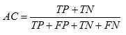
The performance in recognition can be evaluated by following factors: Accuracy (AC), Sensitivity (SE) and Specificity (SP) of detection. They are defined as follows:

1. Classification accuracy is dependent of the number of samples correctly classified.

2. Sensitivity is a proportion of positive cases that are well detected by the test.

3. Specificity is a proportion of negative cases that are well detected by the test.

where, TP is the number of true positives, FP is the number of false positives, TN is the number of true negatives, FN is the number of false negatives.

Figure 4(Fig. 4) show the confusion matrices for the classification results obtained with all three classifiers, SVM, k-NN and Naive Bayes classifier. The confusion matrix is determined between target class and output class. The diagonal cells in each table show the number of cases that were correctly classified, and the off-diagonal cells show the misclassified cases. The blue cell in the bottom right shows the total percent of correctly classified cases (in green) and the total percent of misclassified cases (in red). Gray cells numbered 1 and 2 show sensitivity and specificity, respectively. Gray cells in the third column of Confusion Matrix represent the Precision or Positive Predictive Value (PPV) and Negative Predictive Value (NPV). The positive and negative predictive values are the proportions of positive and negative results in classification tests that are true positive and true negative results. Mathematically, PPV and NPV can be expressed as:

Figure 4. Confusion Matrix composed of information about actual and predicted classifications done by a classification system: (a) SVM classification of breast thermograms, (b) k-NN classification of breast thermograms, (c) Naive Bayes classification of breast thermograms. The diagonal cells represent the number of cases that were correctly classified, while misclassified cases are shown in off-diagonal cells.

Results in confusion matrices indicate that SVM classification results are better than the Naive Bayes classification results, with accuracy ratio of 85% according to 80%, while the best classification result in this research, the accuracy ratio of even 92.5%, is obtained by classifying thermograms using k-NN classifier. High sensitivity (85.7%, 78.6%, 85.7%) and high NPV (91.7%, 89.7%, 90.9%) of SVM, k-NN and Naive Bayes classification indicate that texture features can be parameters for breast cancer screening.

ROC analysis was employed to evaluate the performance of the texture-analysis method in classifying thermography images into positive and negative patterns. In our adduced work, we compared the classification results of three different classifiers. The ROC curve graph in Figure 5(Fig. 5) evinces the accuracy rate of thermograms classification using all three classifiers. In order to predict the accuracy rate of diagnosis, the graphs are plotted between true positive rate and false positive rate.

Figure 5. ROC graph which illustrates the performance of breast thermograms classification using SVM, k-NN and Naive Bayes classifiers. The curve closer to the upper left corner indicates a test with greater accuracy.

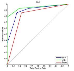
The area under ROC curve (AUC) is a metric that can be used to compare different analysis, in accuracy aspects. The results are considered more precise, when the AUC is large. The area under the curve of k-NN classification, shown in Figure 5(Fig. 5), is the largest, which shows the prediction of the most accurate classification results.

In this study, we present a method to segment thermograms and extract suspected hot regions from the background. Figures 6-8(Fig. 6)(Fig. 7)(Fig. 8) show the extracted hottest regions of four different patients with malignant tumors. The cropped breasts are shown in part (a) of each figure. The hottest regions extraction is simple in cases shown in Figure 6(Fig. 6), while cases shown in Figures 7-8(Fig. 7)(Fig. 8) are more demanding because use of morphological operators is required. Part (b) of each figure shows result of first iteration of minimum variance quantization. Minimum variance quantization can be implemented through several iterations or one iteration with the larger number of quantization levels (colours). A better visibility is provided by using more than one iteration. Part (c) of each figure shows large hot region extracted from original thermograms after first iteration of quantization. Extracted hot region from Figure 8(Fig. 8) has a gap at the place where the temperature of the breast is the highest. Using dilation operator with a geometric template called disc, the gap is removed. Extracted hot region without gap is presented in part (d) of Figure 8(Fig. 8). Figures 6-7(Fig. 6)(Fig. 7) (d) and Figure 8(Fig. 8) (e) show results of second iteration of minimum variance quantization. After the second iteration of quantization, we finally can extract the first and second hottest regions of breast thermograms in the cases shown in Figures 6(Fig. 6) and 8(Fig. 8). These regions are presented in parts (e-f) of Figure 6(Fig. 6) and (f-g) of Figure 8(Fig. 8). Isolated hot regions shown in Figure 7(Fig. 7) (e) contain some undesirable objects that do not belong to potentially suspicious tissue. These objects, incurred as the consequence of warming of the breast due to contact with the body, belong to the edge of the breast. Using erosion operator with a geometric template called disc, all undesirable objects are removed. Figure 7(Fig. 7) (f) shows the isolated first and second hottest regions together. Result of third iteration of minimum variance quantization and the isolated first hottest region are shown in parts (g) and (h) of Figure 7(Fig. 7), respectively. The last two parts of each figure show the first and second hottest regions together and the first hottest region separately, outlined on the original thermograms.

Figure 6. Thermogram of a breast cancer patient 1 and patient 2: (a1, a2) cropped breast, (b1, b2) result of first iteration of minimum variance quantization, (c1, c2) hot region extracted after first iteration, (d1, d2) results of second iteration of minimum variance quantization, (e1, e2) isolated first and second hottest regions, (f1, f2) isolated first hottest region, (g1, g2) first and second hottest regions outlined on the original thermogram, (h1, h2) first hottest region outlined on the original thermogram.

Figure 7. Thermogram of a breast cancer patient 3: (a) cropped breast, (b) result of first iteration of minimum variance quantization, (c) hot region extracted after first iteration, (d) results of second iteration of minimum variance quantization, (e) hot region with undesirable objects extracted after second iteration (f) isolated first and second hottest regions after applying erosion operator, (g) result of third iteration of minimum variance quantization, (h) isolated first hottest region, (i) first and second hottest regions outlined on the original thermogram, (j) first hottest region outlined on the original thermogram.

Figure 8. Thermogram of a breast cancer patient 4: (a) cropped breast, (b) result of first iteration of minimum variance quantization, (c) hot region with gap extracted after first iteration, (d) hot region without gap after applying dilation operator (e) results of second iteration of minimum variance quantization, (f) isolated first and second hottest regions, (g) isolated first hottest region, (h) first and second hottest regions outlined on the original thermogram, (i) first hottest region outlined on the original thermogram.

Conclusion

Thermography is risk-free, pain-free and totally non-invasive, does not involve ionizing radiation and costs less than the other methods for breast screening. Thermal imaging can detect tumorous activity as it begins to develop a blood supply to sustain its growth. Any increased heat from a localized blood supply would suggest pathology. The aim of this research was to make sure that it is possible to use breast thermograms for tumor detection using GLCM features extracted from each thermography image, three different classifiers: SVM, k-NN and Naive Bayes classifier and image segmentation techniques such as minimum variance quantization, dilation of image and erosion of image. The goal of this work was also to compare the classification results of the mentioned three classifiers. Our study indicates that k-NN classifier can be trained to the most effectively classify breast thermograms. Using a k-NN classifier and 20 GLCM features derived from each breast thermogram, we obtained the accuracy ratio of 92.5%, which corresponded to true-positive fraction of 78.6% at a false positive fraction of 0%. Image segmentation plays an important role in many medical imaging applications. We demonstrated that it is possible to successfully extract the tumor region from thermography image of the breast using the combination of different image segmentation techniques such as minimum variance quantization, dilation of image and erosion of image. For the limited number of sample patterns, the experimental results for the breast thermograms are promising. However, a database that covers many more positive cases and negative cases will be needed for training of classifiers in order to apply our method to clinical situations.

Notes

Authors’ contributions

Marina Milosevic, Dragan Jankovic and Aleksandar Peulic share first authorship of this article.

Acknowledgements

Funded by the Serbian Ministry of Education, Science and Technological Development grants: III41007.

References

- 1.Acharya UR, Ng EYK, Tan JH, Sree SV. Thermography based breast cancer detection using texture features and support vector machine. J Med Syst. 2012;36:1503–1510. doi: 10.1007/s10916-010-9611-z. [DOI] [PubMed] [Google Scholar]
- 2.Clausi DA. An analysis of co-occurrence texture statistics as a function of grey level quantization. Can J Remote Sensing. 2002;28:45–62. [Google Scholar]
- 3.EtehadTavakol M, Ng EYK. Breast thermography as a potential non-contact method in the early detection of cancer: a review. J Mech Med Biol. 2013;13:1330001. [Google Scholar]
- 4.EtehadTavakol M, Sadri S, Ng EYK. Application of K- and fuzzy c-means for color segmentation of thermal infrared breast images. J Med Syst. 2010;34:35–42. doi: 10.1007/s10916-008-9213-1. [DOI] [PubMed] [Google Scholar]
- 5.Fok SC, Ng EYK, Tai K. Early detection and visualization of breast tumor with thermogram and neural network. J Mech Med Biol. 2002;2:185–95. [Google Scholar]
- 6.Golestani N, EtehadTavakol M, Ng EYK. Level set method for segmentation of infrared breast thermograms. EXCLI J. 2014;13:241–251. [PMC free article] [PubMed] [Google Scholar]
- 7.Haralick RM, Shanmugam K, Dinstein I. Textural features for image classification. IEEE Trans Syst Man Cybern. 1973 Transactions;3:610–621. [Google Scholar]
- 8.Jakubowska T, Wiecek B, Wysocki M, Drews-Peszynski C Engineering in Medicine and Biology Society, editor. Proceedings of the 25th Annual International Conference of the IEEE, Cancun, Mexico, Sept 17 – 21. Vol. 2. Cancun, Mexico: 2003. Thermal signatures for breast cancer screening – comparative study; pp. 1117–1120. [Google Scholar]
- 9.Keyserlingk JR, Ahlgren PD, Yu E, Belliveau N. Infrared imaging of the breast: initial reappraisal using high resolution digital technology in 100 successive cases of stage I and II breast cancer. Breast J. 1998;4:245–51. doi: 10.1046/j.1524-4741.1998.440245.x. [DOI] [PubMed] [Google Scholar]
- 10.MATLAB and Statistics Toolbox Release 2012. Natick, MA: The MathWorks, Inc; 2012. [Google Scholar]
- 11.Ng EYK. A review of thermography as promising non-invasive detection modality for breast tumour. Int J Therm Sci. 2008;48:849–859. [Google Scholar]
- 12.Ng EYK, Chen Y. Segmentation of breast thermogram: improved boundary detection with modified snake algorithm. J Mech Med Biol. 2006;6:123–136. [Google Scholar]
- 13.Ng EYK, Chen Y, Ung LN. Computerized breast thermography: Study of Image segmentation and temperature cyclic variations. Int J Med Eng Technol. 2001;25:12–6. doi: 10.1080/03091900010022247. [DOI] [PubMed] [Google Scholar]
- 14.Ng EYK, Sudharsan NM. Numerical modelling in conjunction with thermography as an adjunct tool for breast tumour detection. BMC Cancer. 2004;4:1–26. doi: 10.1186/1471-2407-4-17. [DOI] [PMC free article] [PubMed] [Google Scholar]
- 15.Ng EYK, Ung LN, Ng FC. Statistical analysis of healthy and malignant breast thermography. J Med Eng Technol. 2001;25:253–63. doi: 10.1080/03091900110086642. [DOI] [PubMed] [Google Scholar]
- 16.Pakhira MK. A modified k-means algorithm to avoid empty clusters. Int J Rec Trends Engin. 2009;1:220–226. [Google Scholar]
- 17.Soh LK, Tsatsoulis C. Texture analysis of SAR sea ice imagery using gray level co-occurrence matrices. IEEE Trans Geosci Remote Sensing. 1999;37:780–795. [Google Scholar]
- 18.Sowmya B, Bhattacharya S. Colour image segmentation using fuzzy clustering techniques and competitive neural network. Appl Soft Computing. 2011;11:3170–8. [Google Scholar]
- 19.Tan JH, Ng EYK, Acharya UR. Study of normal ocular thermogram using textural parameters. Infrared Phys Technol. 2010;53:120–6. [Google Scholar]
- 20.Vapnik V. Statistical learning theory. New York: Wiley; 1998. [Google Scholar]
- 21.Wishart GC, Campisi M, Boswell M, Chapman D, Shackleton V, Iddles S, et al. The accuracy of digital infrared imaging for breast cancer detection in women undergoing breast biopsy. Eur J Surg Oncol. 2010;36:535–540. doi: 10.1016/j.ejso.2010.04.003. [DOI] [PubMed] [Google Scholar]
- 22.Zhang H. 17th International Florida Artificial Intelligence Research Society Conference (FLAIRS 2004) Palo Alto, CA: AAAI Press; 2004. The optimality of naive Bayes; p. 562–7. [Google Scholar]