

Abstract
Spatial normalization is a crucial step in assessing patterns of neuroanatomical structure and function associated with health and disease. Errors that occur during spatial normalization can influence hypothesis testing due to the dimensionalities of mapping algorithms and anatomical manifolds (landmarks, curves, surfaces, volumes) used to drive the mapping algorithms. The primary aim of this paper is to improve statistical inference using multiple anatomical manifolds and Large Deformation Diffeomorphic Metric Mapping (LDDMM) algorithms. We propose that combining information generated by the various manifolds and algorithms improves the reliability of hypothesis testing. We used this unified approach to assess variation in the thickness of the cingulate gyrus in subjects with schizophrenia and healthy comparison subjects. Three different LDDMM algorithms for mapping landmarks, curves and triangulated meshes were used to transform thickness maps of the cingulate surfaces into an atlas coordinate system. We then tested for group differences by combining the information from the three types of anatomical manifolds and LDDMM mapping algorithms. The unified approach provided reliable statistical results and eliminated ambiguous results due to surface mismatches. Subjects with schizophrenia had non-uniform cortical thinning over the left and right cingulate gyri, especially in the anterior portion, as compared to healthy comparison subjects.
Keywords: Large Deformation Diffeomorphic Metric Mapping (LDDMM), the Laplace-Beltrami Operator, Gaussian Random Field, cingulate gyrus, cortical thickness, schizophrenia
1. Introduction
In recent years, computational algorithms have been developed to compare functions of the cortical mantle in human subjects with and without neuropsychiatric disease using high-resolution magnetic resonance (MR) imaging datasets. The most popular approach for making such comparisons is to spatially normalize the neuroanatomical structure, carry relevant functions (e.g. cortical thickness, functional response) onto atlas coordinates, and then to perform hypothesis testing in the atlas space. We refer to this approach as extrinsic since it depends on the relationship between individual brains and an external atlas (Vaidyanathan et al., 1997, Csernansky et al., 1998, Grenander and Miller, 1998, Thompson et al., 1998, Fischl et al., 1999a, Fischl et al., 1999b, Fischl and Dale, 2000, Csernansky et al., 2002, Chung et al., 2003, Gee et al., 2003, Chung et al., 2004, Csernansky et al., 2004a, Csernansky et al., 2004b, Thompson et al., 2004, Van Essen, 2004a, Van Essen, 2004b, Chung et al., 2005, Miller et al., 2005, Thompson et al., 2005, Van Essen, 2005).
The field of computational anatomy (CA) has three aims: (a) construction of anatomical manifolds, such as landmarks, curves, surfaces, and subvolumes; (b) construction of anatomical correspondences across subjects; (c) statistical codification of anatomical functions via probability measures allowing for inference and hypothesis testing related to disease states. The automated construction of anatomical manifolds that is receiving tremendous attention by many groups has facilitated analyses of brain structure in populations with and without neuropsychiatric disease. Deformable and active models as well as statistical models are being used to generate 1-dimensional manifold curves in R2 or R3 and 2-dimensional manifold surfaces, and to segment anatomical volumes into 3-dimensional submanifolds (Bakircioglu et al., 1998, Dale et al., 1999, Xu et al., 1999, MacDonald et al., 2000, Miller et al., 2000, Fischl et al., 2002, Han et al., 2002, Ratnanather et al., 2003, Han et al., 2004, Xu et al., 2004, Khan et al., 2005). Local coordinate representations of cortical manifolds have included both spherical and planar representations for local coordinates in studying the brain (Fischl et al., 1999a, Van Essen, 2002, Hurdal and Stephenson, 2004, Tosun et al., 2004, Van Essen, 2004a, Wang et al., 2005a, Wang et al., 2005b, Wang et al., 2005c). To compare anatomical manifolds in various populations, one has to account for the fundamental structural variability of biological shapes. The earliest mapping of biological coordinates via landmarks and dense imagery was pioneered in the early 1980s and continues today by Bookstein and Bajcsy, Gee and co-workers (Bookstein, 1978, Bajcsy et al., 1983, Dann et al., 1989, Bookstein, 1991, Gee et al., 1993, Bookstein, 1996, Bookstein, 1997, Avants and Gee, 2003, Chen et al., 2003, Avants and Gee, 2004). Mappings restricted to the cortical manifold have been computed through spherical representations of the cortical manifold or landmarks or curves (Thompson et al., 1996, Fischl et al., 1999a, Joshi and Miller, 2000, Van Essen, 2002, Tosun et al., 2004, Van Essen, 2005). Using such mappings in combination with statistical representations of shapes and other functions, CA studies of normal brain growth, aging, and neuropsychiatric diseases have rapidly expanded over the past ten years (Csernansky et al., 2004b, Thompson et al., 2004, Thompson et al., 2005). However, recent CA studies have raised issues about the effects of anatomical mapping methods on statistical hypothesis testing. In general, prior research has suggested that high dimensional mapping methods increase power of hypothesis testing in part by increasing the accuracy of spatial normalization (Desai et al., 2005, Miller et al., 2005, Kirwan et al., 2006, Vaillant et al., 2007).
Our own efforts in CA have been largely focused on the generation of anatomical manifolds (landmarks, curves, surfaces, subvolumes) and on the development of high dimensional mapping algorithms for them. Large deformation diffeomorphic metric mapping (LDDMM) is one of these algorithms and provides one-to-one, smooth (forward and inverse) transformations φ ∈ G acting on the ambient space φ : X ⊂ R3 → X. Thus, connected sets remain connected, disjoint sets remain disjoint, and the smoothness of neuroanatomical features such as curves and surfaces is preserved. These transformations are generated by the flow of diffeomorphisms so that they are not additive and provide guaranteed bijections between anatomical configurations. The length of the optimal flow trajectory connecting two anatomical configurations gives a metric distance that can be used to quantify the “closeness” in shape between different instances. Thus far, we have developed techniques in the LDDMM framework used for treating image datasets, including 3D volumetric image matching, multi-value vector image matching, tensor image matching (Beg et al., 2004, Beg et al., 2005, Cao et al., 2005), and point-based matching (Joshi and Miller, 2000, Glaunes et al., 2004a, Glaunes et al., 2004b, Allassonniere et al., 2005, Vaillant and Glaunes, 2005, Glaunes et al., 2007). These implementations of the point-based LDDMM deal with various configurations of points, curves and surfaces (Joshi and Miller, 2000, Glaunes et al., 2004a, Glaunes et al., 2004b, Vaillant and Glaunes, 2005). The applications of LDDMM mapping algorithms in studies of brain structure and function have shown their power for detecting functional activation and the effects of various neuropsychiatric diseases, especially in their mildest forms (Wang et al., 2001, Csernansky et al., 2002, Csernansky et al., 2004a, Csernansky et al., 2004b, Miller et al., 2005, Kirwan et al., 2006, Wang et al., 2006, Qiu et al., 2007).
While extrinsic analysis has many advantages, high individual brain variability combined with the essential demand for spatial normalization may introduce errors that directly influence the testing of statistical inferences. Also, because of the complexity of the human cortical mantle, one-to-one correspondences between anatomical configurations across subjects may not be easily defined. For example, when cortical surfaces are highly curved, different anatomical correspondences across subjects could be found depending on the different types of anatomical manifolds that drive the mapping algorithms; i.e., landmarks, curves, and surfaces. Thus, the statistical conclusion may depend on manifolds that are used to estimate the anatomical correspondences (Desai et al., 2005).
In this paper, we compare multiple LDDMM mapping algorithms driven by a variety of anatomical manifolds (landmarks, curves, surfaces, and volumes), and then present a framework for combining the information derived from these manifolds to perform hypothesis testing. This framework combines the information from the available anatomical manifolds into a single statistical model so that abnormalities associated with a disease condition common to all of the mappings are identified. We demonstrate that this framework improves the reliability of hypothesis testing by eliminating errors caused by the registration of different modalities of anatomical manifolds. Our approach is similar in concept to recent brain tissue segmentation methods that use multi-modality images that feature both common and complementary information.
We defined disease-related functions, F(x), on the surface of the cingulate gyrus represented by 0,1 and 2 dimensional manifolds (landmarks, curves, surfaces). We compared separate LDDMM mappings of landmarks, curves, and surfaces to determine what information of the cortical surface was taken into account in each of the three mapping algorithms. The correspondence between the template and the target cortical surfaces were represented by diffeomorphic maps of φL (landmark), φC (curve), and φS (surface) respectively. Due to differences in the dimensionality of landmarks, curves, and surfaces, φL, φC, and φS are not identical for a single subject. As a consequence, the representation of F(x) in the atlas depends on which diffeomorphic map is chosen; i.e., the variation due to the mapping algorithm is introduced into F(x) in the atlas. We modeled this variation as a random effect in our statistical testing. For this, we first built a Gaussian Random Field (GRF) model of the function using decomposition over the eigenfunctions of the Laplace-Beltrami operator in the atlas for each of the mappings. We then tested inferences related to both diagnosis and mapping methods on GRFs via a linear regression model. We finally applied this framework to a comparison of the pattern of variation in the thickness of the cingulate gyrus in groups of subjects with and without schizophrenia.
We selected the cingulate gyrus for this study because of prior studies suggesting that subjects with schizophrenia show thinning of this structure (Narr et al., 2005) and because patterns of individual variation in its sulcal/gyral patterning have been relatively well defined (Ono et al., 1990, Fornito et al., 2006a, Fornito et al., 2006b). We fully explore the generation of anatomical manifolds of landmarks, curves, and surfaces in the cingulate gyrus and the matching error of each mapping algorithm. Our results empirically show that statistical testing is dependent on the mapping algorithms and that the combination of anatomical manifold information via diffeomorphic mappings provides a reliable approach for evaluating the statistical significance of results. In our comparison of subjects with and without schizophrenia, our results suggest that schizophrenia is characterized by a heterogeneous pattern of thinning throughout both the left and right cingulate gyri.
2. Large Deformation Diffeomorphic Metric Mapping (LDDMM)
Two cortical surfaces may be mapped onto each other by treating the 2-dimensional manifolds of the cortical surfaces as 0-dimensional information (landmark points), or 1-dimensional features (curves), or 2-dimensional structure of the manifold as a whole. An advantage to 0-dimensional and 1-dimensional manifolds is that the computation is reduced compared to 2-dimensional surface matching. Also the selection of landmarks and curves can be guided by previous knowledge derived from postmortem studies. In the setting of LDDMM, we developed mapping algorithms that utilize three different anatomical manifolds; i.e. landmarks, curves, and surfaces (Joshi and Miller, 2000, Vaillant and Glaunes, 2005, Glaunes et al., 2007). All of these mapping algorithms provide diffeomorphic maps --- one-to-one, reversible smooth transformations that preserve topology. The use of LDDMM for studying the shapes of objects requires the placement of shapes in a metric space, provides a diffeomorphic transformation, and defines a metric distance that can be used to quantify the similarity between two shapes. We assume that the shapes can be generated one from the other via a flow of diffeomorphisms, solutions of ordinary differential equation = νt(φt), t ∈[0,1] with φ0 = id, identity map, and associated velocity fields νt. For a pair of objects Itemp and It arg, a diffeomorphic map φ transforms one to the other φ1 · Itemp = It arg at time t = 1. The metric distance between shapes is the length of the geodesic curves φt · Itemp,t ∈ [0,1] through the shape space generated from connecting Itemp to It arg in the sense that φ1 · Itemp = It arg. The metric ρ(Itemp, It arg) between two shapes Itemp and It arg takes the form
where νt ∈ V, a Hilbert space of smooth vector fields with norm ∥·∥V to ensure that the solutions are diffeomorphisms. In practice, the metric ρ and the diffeomorphic map φ between Itemp and It arg are computed via a variational problem:
| (1) |
where D(φ1 · Itemp, It arg) quantifies the closeness between the deformed object φ1 · Itemp and object It arg. Such a variational problem can be adapted to different objects, such as images, vectors, tensors, landmarks, curves, and surfaces (Joshi and Miller, 2000, Beg et al., 2004, Glaunes et al., 2004a, Beg et al., 2005, Cao et al., 2005, Vaillant and Glaunes, 2005, Glaunes et al., 2007, Vaillant et al., 2007). For the purpose of registering two cortical surfaces, we review how to define D(φ1 · Itemp, It arg) for objects of landmarks, curves, and surfaces.
2.1 LDDMM-landmark
A point in R3 is characterized by its location in R3. The closeness of two points can be quantified by the Euclidean distance between them. Assume {xi, yi} be a pair of landmarks, where xi ∈ Itemp and yi ∈ It arg for i = 1,2,…,N. We define D(φ1 · Itemp, It arg) as
which quantifies mismatching between two corresponding points (Joshi and Miller, 2000).
2.2 LDDMM-curve
Since a curve is a geometric object, it cannot be uniquely reconstructed based on the locations of a set of points. We consider that a curve embedded in R3 is a one-dimensional manifold in the sense that the local region of every point on the curve is equivalent to a line which can be uniquely defined by this point and the tangent vector at this location (Glaunes et al., 2007). Therefore, in the discrete case, we represent a curve with a sequence of points and tangent vectors, I = {cl, τl}, where is the center of two consequent points xl1 and xl2 and τ = xl2 − xl1 approximates the tangent vector at cl.
Now we define D(φ1 · Itemp, It arg) for registering two curves in the LDDMM setting based on their position and tangent vectors. Let Itemp = {cl, ηl} and It arg = {ch, ηh} be template and target curves represented by centers of two consequent points on the curve and their corresponding tangent vectors. Denote the deformed template curve φ1 · Itemp = {cl1, ηl1}, where is the center of points φ1 · xl1 and φ1 · xl2, τl1 = φ1 · xl2 − φ1 · xl1 is the tangent vector at location cl1. Let l, g be indices of points on the curve Itemp and h, q be indices of points on the curve It arg. The data attachment term D(φ1 · Itemp, It arg) in Eq. (1), which quantifies the closeness of the two curves φ1 · Itemp and It arg, is given in the form
where kW(x, y) is a kernel and in practice defined as an isotropic Gaussian kernel matrix, . ∥x − y∥ denotes Euclidean distance between points x and y and id3×3 is a 3 × 3 identical matrix. The first two terms are intrinsic energies of the two curves φ1 · Itemp and It arg. It is clear that D(φ1 · Itemp, It arg) does not require two curves with equal number of points and dense correspondence between the matched curves. Roughly, the more rounded the curves are, the higher energy they possess; i.e., flat shaped parts of the curves tend to vanish in the space of this measure. The last term gives penalty to mismatching between tangent vectors of It arg and those of φ1 · Itemp.
2.3 LDDMM-surface
We assume the cortical surface embedded in R3 to be a two-dimensional manifold in the sense that the neighborhood of every point on the surface is equivalent to a two-dimensional plane in Euclidean space. Such a plane can be uniquely defined by a point and a vector originated at this point and normal to the plane. Therefore, we can represent a triangulated mesh as I = {cf, ηf}, a set of points and normal vectors, where is the center of triangle f on I with three vertices xf1, xf2, xf3 and is the normal vector to f at location cf. The symbol × denotes cross product (Vaillant and Glaunes, 2005, Vaillant et al., 2007).
Now we define D(φ1 · Itemp, It arg) for registering surfaces in the LDDMM setting based on their position and normal vectors. Let Itemp = {cf,ηf} and It arg = {ch,ηh} be the template and target triangulated meshes represented by center points of triangles on the surface and their corresponding normal vectors. Denote the deformed template surface φ1 · Itemp = {cf1,ηf1}, where is the center of deformed triangle f and is the normal vector to deformed triangle f at location cf1. Let f, g be indices of triangles on the surface Itemp and h, q be indices of triangles on the surface It arg. The data attachment term D(φ1 · Itemp, It arg) in Eq. (1), which quantifies the closeness between φ1 · Itemp and It arg, is given in the form
This term in the LDDMM-surface mapping is similar to that in the LDDMM-curve mapping, except the surface is represented by its normal vector while the curve is by its tangent vector.
3. Statistical Analysis
To test for a group difference in cortical thickness, we assumed that our observations arose from random processes, including anatomical structure M (cortical surface) and thickness map F indexed over M. The variation in anatomical structure relative to the atlas Matlas was carried by diffeomorphic maps φ such that φ · M = Matlas. In our case, φ was generated by the LDDMM landmark, or curve, or surface mapping algorithms, respectively denoted by φL, φC, and φS. Next, we represented anatomical structure through the anatomical atlas coordinate system Matlas and the diffeomorphic map φ and considered φ as a nuisance parameter in our statistical analysis. In the anatomical atlas coordinates, F was modeled as a Gaussian random field (GRF) and characterized by an infinite number of Gaussian random variables Fi defined as
| (2) |
where ν(x) is area measure at location x ∈ Matlas and ψi(x) is a basis function indexed over Matlas. We chose ψi(x) to be the i th eigenfunction of the Laplace-Beltrami (LB) operator on Matlas, the extension of the Laplacian from the regular grid to an arbitrary surface. The LB operator was characterized by intrinsic surface geometric information, such as length, area and angle between two curves on the surface so that the LB eigenfunctions in Eq.(2) were only dependent on the geometry of the extrinsic atlas and not on thickness data (Qiu et al., 2006). Figure 1 illustrates the first eight LB eigenfunctions on the left cingulate surface. Red and blue respectively denote regions with positive and negative values. These eigenfunctions are similar to sine or cosine basis functions on the regular grid in the sense that the positive and negative regions alternate more rapidly when moving to the higher order of basis. For instance, the first eigenfunction is constant everywhere and its corresponding coefficient F1 represents the average thickness over the cingulate surface. In turn, the second eigenfunction has the waveform from negative to positive as it moves from the anterior to the posterior extreme of the cingulate gyrus. F2 represents amount of signal of F(x) in the same pattern as ψ2(x).
Figure 1.

Panels (a-f) respectively show the first eight eigenfunctions of the Laplace-Beltrami operator on the left template cingulate surface.
We aimed to produce a test that could identify the LB eigenfunctions that significantly contributed to group differences in thickness. We assumed that the finite number of Fi carried enough information so that we could perform statistical analysis on them. In general, only one mapping approach is needed to derive Fi with diagnosis as the main factor in a statistical analysis. However, Eq. (2) implies that Fi depends on the estimated diffeomorphic map φ. Therefore, both diagnosis and mapping algorithms need to be considered as main factors in hypothesis testing. Our statistical task was to integrate anatomical manifold information relating to landmarks, curves, surfaces so that the effects of both diagnosis and mapping algorithm on F(x) could be examined. To do so, we associated the ith LB eigenfunction with a set of coefficients where were computed from Eq. (2), respectively, based on the landmark, curve, and surface mappings. were thus included as dependent variables in the statistical analyses using a linear regression model. Diagnostic group and mapping algorithm were included as categorical predictor variables while covarying for total cerebral volume. For each subject, the coefficients from the three mapping were considered as repeated measures, and the error term in the linear regression model was split into errors between and within subjects. Interactions between diagnosis and mapping algorithm were also examined.
As a comparison with statistical testing using a unified approach, we also performed a linear regression analysis to test for the effects of diagnosis on the first ten Fi when one mapping algorithm was applied. Each individual coefficient was separately examined and considered as a dependent variable in the statistical analysis using a linear regression model. Diagnostic group (schizophrenia subjects and comparison subjects) was included as a categorical predictor variable covarying with total cerebral volume. A similar statistical model was used to examine diagnostic group differences in Fi for every mapping algorithm.
4. Cingulate Thickness Variation in Schizophrenia
4.1 Subjects and Image Acquisition
Forty-nine individuals with schizophrenia and sixty-four healthy comparison subjects, group-matched for age, gender, race, and parental socioeconomic status, gave written informed consent for participation in this study after the risks and benefits of participation were explained to them. Individual demographic and clinical information have been detailed elsewhere (Csernansky et al., 2004a). All subjects with schizophrenia were outpatients and were scanned after they had been optimally treated with antipsychotic drugs and attained clinical stability.
MR scans were collected on a Magnetom SP-4000 1.5-Tesla Siemens imaging system with a standard head coil using a turbo-FLASH sequence (TR=20ms, TE=5.4ms, flip angle=30 degrees, 180 slices, 256-mm field of view, matrix=256×256, number of acquisitions=1, scanning time=13.5min) that acquired three-dimensional datasets with 1mm3 isotropic voxels across the entire cranium (Venkatesan and Haacke, 1997).
4.2 Cingulate Manifold Generation
The cingulate surfaces were then represented by landmarks, curves, and surfaces in order to apply LDDMM landmark, curve, and surface mappings, respectively.
Surfaces
Bayesian segmentation using the expectation-maximization algorithm to fit the compartmental statistics was used to label voxels in the subvolume as gray matter (GM), white matter (WM), or cerebrospinal fluid (CSF) (Joshi et al., 1999, Miller et al., 2000). Then, surfaces were generated at the GM/WM interface using a topology-correction method and a connectivity-consistent isosurface algorithm (Han et al., 2002). The cingulate gyrus was delineated by tracking principal curves via dynamic programming (Ratnanather et al., 2004).
Curves
Two sets of curves, exterior and interior, were delineated on the cingulate manifold surfaces via dynamic programming (Khaneja et al., 1998, Ratnanather et al., 2004). The exterior curves were already defined in the process of delineating the cingulate manifold surface (Wang et al., 2007) by following the external boundary of the cingulate manifold surface formed by callosal sulcus, cingulate sulcus, subpariteal sulcus and calcarine sulcus, as labeled as curves 1,2 3 on the template cingulate surface in Figure 2(a). The interior curves followed the foldings of the cingulate manifold surface in its interior space, marked as curves 4,5,6 in Figure 2(a).
Figure 2.

Panel (a) show six curves colored differently on the left template cingulate surface. Three exterior curves are labeled as 1,2,3 in white; three interior curves are marked as 4,5,6 in black. Panel (b) illustrates seventy two landmark points.
Landmarks
Corresponding landmarks were extracted as the result of matching above template and subject curves via (Bakircioglu et al., 1998) where distances between curves followed the Frenet representation of speed, curvature and torsion. Examples of these landmarks on the template surface are illustrated in Figure 2(b).
4.3 LDDMM Mappings
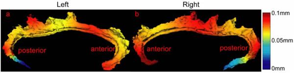
We chose the left and right cingulate gyri as represented in the MR scan collected from one of the healthy comparison subjects as a template and mapped all other anatomies to this template via LDDMM landmark, curve, and surface mappings. To evaluate the precision of these mappings, we computed distances between the deformed surfaces and the template surface. Let νSi and νTj respectively be vertices on deformed surface S and template surface T. The distance of νTj to S is defined as , where ∥·∥ is the Euclidean distance in R3. We call dTj, a function indexed over the template surface; i.e., a distance error map that quantifies the mismatching error at each location of the template.
Left and right columns in Figure 3 show average distance error maps from 112 deformed surfaces generated by landmark, curve, and surface mappings. Large mismatching errors occurred on the boundary of the cingulate gyri on both the left and right sides and with the use of all three mapping algorithms. Larger mismatching errors appeared in the very anterior and posterior regions of the left and right cingulates with the use of the landmark and curve mapping algorithms, possibly because paired landmarks and curves do not contain enough information to represent the complexity of the anatomical structure in these areas. When reducing 2-dimensional surfaces to sets of 0-dimensional points or 1-dimensional curves, geometric information of the cortical surface is discarded. Moreover, due to the discretization of these appoaches, there may not always be homologous points on two cortical surfaces, which gives also constrains the registration processes. Compared with these two mapping algorithms, most of mismatching distance errors of the surface mapping algorithm were less than 1 mm as shown in Figure 3(c,f). However, error can still be introduced when complex anatomical structures do not offer one-to-one correspondences across subjects. As an example of this problem, the cingulate sulcus has an interrupted course (Ono et al., 1990, Fornito et al., 2006a), which produces two (or more) distinct segments (cingulate and paracingulate).
Figure 3.

Panels (a,b,c) show average distance error maps over 112 deformed left cingulate surfaces for the landmark, curve, and surface mappings, respectively. Similarly, panels (d,e,f) show average distance error maps over 112 deformed right cingulate surfaces.
We excluded paracingulate portion in our study if it was present. As shown in Figure 4, the cingulate gyrus in panel (a) is relatively small when the paracingulate presents compared to one in panel (b) without appearance of the paracingulate. Since the portion in the red frame of Figure 4(b) has no corresponding surface in Figure 4(a), the LDDMM-surface cannot provide an accurate correspondence between these two anatomies. One approach for improving the quality of the LDDMM-surface matching in such cases is to include the input of an expert, such as was done during the manual placement of landmarks or curves. However, the results of all three approaches to mapping a given cortical surface (landmark, curve, and surface matchings) must eventually be combined for hypothesis testing.
Figure 4.
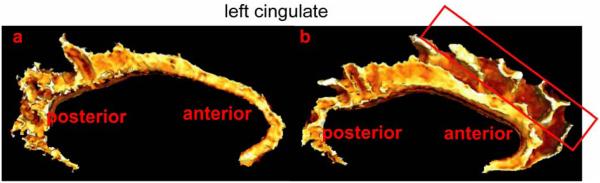
Panels (a,b) show left cingulate structures. The cingulate in panel (a) is relatively narrow due to the appearance of the paracingulate that is excluded in the study. The region in the red frame of panel (b) has no similar structure in the cingulate gyrus in panel (a).
4.4 Cortical Thickness Map
We indexed the thickness of the cingulate gyrus as a function over the local coordinates of the cortical surface using Local Labeled Cortical Mantle Distance Map (LLCMDM), a modification of LCMDM developed by (Miller et al., 2003). LLCMDM is a refinement of LCMDM in that it is designed for the analysis of a cortical surface instead of a image volume. LLCMDM labels each vertex on the GM/WM surface in relationship to a set of GM voxels. Hence, LLCMDM forms a secondary data structure of the same dimension as the GM/WM surface and associate each vertex with a set of labeled pairs {(x, d)}: S → {(l(x(νi)), d(x(νi))|l(x(νi)) = GM}, d(x(νi)) and l(x(νi)) representing the distances of the voxel center x(νi) to vertex νi on the cortical surface and the associated tissue type of voxel x(νi). From LLCMDM-derived measures of cortical GM distribution, we calculated via the histogram of d(x(νi)) the total number of GM as a function of distance from νi and its neighbor. Then, the thickness at νi was quantified using the 95 percentile of the histogram, which mitigates any error caused by tissue misclassification at a significance level α = 0.05.
Figure 5(a) shows the cortical thickness maps of the left and right cingulate gyri in two healthy comparison subjects, selected from the available comparison sample. The maps suggest that thickness is non-uniformly distributed over the cingulate surface; i.e., the anterior segment of the cingulate is thicker than the posterior segment and the gyral region is thicker than the sulcal region. Figure 5(b) gives examples of thickness maps of the left and right cingulate gyri in two individuals with schizophrenia, again selected from the available sample of schizophrenia subjects. In these subjects, thickness varied over the cingulate surface in a manner that was similar to the healthy comparison subjects, and yet, thickness appeared to be reduced overall across the cingulate surfaces as compared to the healthy individuals.
Figure 5.

Panel (a) shows cortical thickness maps of two healthy subjects, while panel (b) illustrates thickness maps of two schizophrenic subjects. Each row shows thickness maps on the left and right cingulates of one subject. In each panel, the top row shows the thickness maps of the subject with large median thickness value in the right cingulate while the bottom row shows the thickness maps of the subject with small median thickness value in the right cingulate.
Figure 6 shows average thickness maps of the left and right cingulate surfaces in groups as defined by diagnosis (rows (a,d) for the comparison group, and rows (b,e) for the schizophrenia group). Average thickness maps were similar for the three mapping algorithms in both groups and resembled the cortical thickness maps of the individuals shown in Figure 5. However, average thickness maps constructed using the landmark and curve mappings showed fewer differences in the anterior and posterior extremes of the cingulate gyrus than those constructed using surface mapping. Standard deviations for cortical thickness measurements in Figure 7 are similar across the groups and mapping algorithms. The very anterior and posterior segments of the left and right cingulate gyri showed greater variation in thickness partly due to mapping error as shown in Figure 3. The curve mapping algorithm produced the largest deviation in thickness in both of these regions, while the surface mapping algorithm produced the smallest deviation. The average difference in the cortical thickness between diagnostic groups are indexed in color in rows (c,f) in Figure 6. Red denotes thicker regions in the healthy comparison group and blue denotes thicker regions in the schizophrenia group.
Figure 6.

Rows (a-b) show the average thickness maps of the left cingulate in the control (row (a)) and schizophrenic (row (b)) groups. The average group difference in thickness of the left cingulate is shown in row (c). Similarly, rows (d-e) show average thickness maps of the right cingulate in the control (row (d)) and schizophrenic (row (e)) groups. The average group difference in thickness of the right cingulate is shown in row (f). From the left to the right columns, the average thickness maps were generated via the landmark, curve, and surface mappings, respectively.
Figure 7.

Rows (a-b) show the standard deviation maps of the thickness for the left cingulate in the control (row (a)) and schizophrenic (row (b)) groups. Similarly, rows (c-d) show the standard deviation maps of the thickness for the right cingulate in the control (row (c)) and schizophrenic (row (d)) groups. From the left to the right columns, the standard deviation maps were generated via landmark, curve, and surface mappings, respectively.
4.5 Statistical Results via Unifying the Three Mappings
We tested each of the coefficients associated with the first ten LB eigenfunctions using a linear regression model with diagnosis and mapping method as independent variable after covarying for total cerebral volume. Coefficients from the first, seventh and eighth LB eigenfunctions in the left cingulate gyrus show significant effects of diagnosis after covarying for total cerebral volume (the second column in Table 1). This indicates that the group differences shown in the three panels of Figure 6 (c) can be represented by these eigenfunctions after considering the variability of thickness values due to individual variability and mapping errors. In the right cingulate, coefficients from the first and sixth LB eigenfunctions show significant effects of diagnosis after covarying for total cerebral volume (the sixth column in Table 1). This suggests that the common characteristics of the thickness group differences shown in the three panels of Figure 6(f) can be represented by these eigenfunctions after considering the variability of thickness values due to individual variability and mapping errors.
Table1.
Table lists p-values for diagnostic effect on coefficients. Significant (p<0.05) or near-significant effect of diagnosis (0.05<p<0.1) are shown in bold face after covarying for total cerebral volume.
| the i th coefficient |
Left | Right | ||||||
|---|---|---|---|---|---|---|---|---|
| combined | landmark | curve | surface | combined | landmark | curve | surface | |
| 1 | 0.0455 | 0.0580 | 0.0590 | 0.0433 | 0.0069 | 0.0180 | 0.0027 | 0.0248 |
| 2 | 0.7450 | 0.9468 | 0.9906 | 0.3729 | 0.4645 | 0.3363 | 0.9885 | 0.1738 |
| 3 | 0.7414 | 0.4305 | 0.2880 | 0.1708 | 0.9400 | 0.8252 | 0.5882 | 0.3428 |
| 4 | 0.3660 | 0.7027 | 0.3923 | 0.2858 | 0.1224 | 0.1352 | 0.1911 | 0.2429 |
| 5 | 0.1266 | 0.3924 | 0.0972 | 0.1621 | 0.1530 | 0.2313 | 0.2623 | 0.2773 |
| 6 | 0.9205 | 0.7067 | 0.9494 | 0.4743 | 0.0390 | 0.1091 | 0.0713 | 0.0390 |
| 7 | 0.0492 | 0.0916 | 0.1659 | 0.0445 | 0.1643 | 0.4270 | 0.0826 | 0.3725 |
| 8 | 0.0494 | 0.0110 | 0.1587 | 0.7764 | 0.8109 | 0.7869 | 0.7171 | 0.9500 |
| 9 | 0.7046 | 0.9618 | 0.7133 | 0.0746 | 0.9194 | 0.9025 | 0.6824 | 0.3145 |
| 10 | 0.3108 | 0.8355 | 0.6997 | 0.0220 | 0.9042 | 0.9762 | 0.7469 | 0.9741 |
To illustrate the effects of diagnosis on thickness as represented by the unified method, we reconstructed maps of the significant group differences in thickness by first subtracting the mean of all coefficients generated by the three mappings in the schizophrenia group from the mean of all coefficients in the healthy comparison group, and then multiplying the difference by its associated LB eigenfunction. Figure 8 shows the effects of diagnosis on thickness of the left and right cingulate gyri. The effect of diagnosis in the left cingulate (panel a) was constructed using the first, seventh, and eighth LB eigenfunctions, while the effect of diagnosis in the right cingulate (panel b) was constructed using the first and sixth LB eigenfunctions. The results of the visualization in Figure 8 suggest that the identified combinations of LB eigenfunctions can be used to represent group differences in the thickness over the left and right cingulate gyri. Also, this visualization suggests that the pattern of thinning of the cingulate gyrus is variable along its anterior-posterior axis in individuals with schizophrenia, with the most posterior segment of the cingulate being less affected.
Figure 8.
Diagnostic group differences in thickness are reconstructed from the LB eigenfunctions associated with the coefficients showing statistically significant effects of diagnosis.
4.6 Comparison of Statistical Results Derived from Single and Unified Mappings
To compare the results obtained using the unified method with the results obtained using the three individual mappings, we examined the effects of diagnosis on coefficients of the LB eigenfunctions using each of three mapping algorithms after covarying for total cerebral volume. The statistical results from each mapping algorithm (Table 1) were in reasonable agreement. Both the left and right cingulate gyri exhibited similar patterns of cortical thickness variation and the calculated eigenfunctions with their associated coefficients yielded similar patterns of significant effects of diagnosis. However, the three different mapping algorithms also produced some discrepant statistical results. For instance, the seventh coefficient of the left cingulate showed a significant effect of diagnosis when using the landmark and surface mappings at significant level of α = 0.05, but not when using the curve mapping. Also, the eighth coefficient showed a significant effect of diagnosis when using the landmark mapping, but not when using the curve or surface mapping. These results support the need for an approach to hypothesis testing that can integrate the results from all the three mappings. Compared with the statistical testing using each mapping algorithm in turn, the statistical testing after combining the three mappings produced the most reliable results regarding the effects of diagnosis on thickness; i.e., these results were most similar to the results obtained when using the surface mapping algorithm with the smallest matching error.
After considering statistical comparisons derived from each mapping algorithm as a set of statistical tests, we used the Bonferroni correction to lower significance level of α in order to avoid a lot of spurious positives, which sets . In this case, the eighth LB eigenfunction showed a significant diagnostic effect on the thickness in the left cingulate when using the landmark mapping, while the first LB eigenfunction showed significant diagnostic effect on the thickness in the right cingulate when using the curve mapping. Compared with these results, the statistical testing after combining the three mappings increased the statistical power.
5. Discussion
In this paper, we present a statistical framework for combining anatomical manifold information from three different diffeomorphic mappings to study abnormalities in brain structure and function in clinical populations. By diminishing errors associated with any single mapping approach, this method improved our ability to identify and characterize abnormalities in the structure of the cingulate gyrus in subjects with schizophrenia. We believe that this framework should also be helpful in characterizing irregularities of the cortex in subjects with other neuropsychiatric disorders.
Existing approaches for detecting group differences in functions defined on brain anatomical structure across clinical populations generally include two steps. The first step is to apply a mapping algorithm, which is in general based on single modality of anatomical manifold, to transform brains into an extrinsic common coordinate system. Then, the second step is to test inferences on the functions in the extrinsic common coordinates. The difficulty with any extrinsic strategy is that the one to one correspondence between anatomical configurations across subjects may not always be well defined (as the example shown in Figure 4). Furthermore, for highly curved cortical surfaces, different anatomical correspondences across subjects could be found based on different types of anatomical manifolds, such as landmarks, curves, and surfaces. These limitations imply that the statistical conclusion from any extrinsic analysis will depend on the algorithm that is used to estimate the anatomical correspondence. Our results support this assertion in that they demonstrate that the use of different mapping algorithms had substantial effects of the conclusions drawn from statistical testing. This may be partly due to artificial variation in thickness values at particular locations within a cortical region caused by matching errors. Anatomical manifolds with higher dimensionality appear to produce more accurate matching. For instance, the LDDMM surface matching algorithm produced relatively smaller matching errors, and showed the least deviation of thickness across the populations being studied. However, combining the results of the three mapping algorithms further mitigated variability in thickness values due to matching error, and allowed us to define features of cortical thinning in the individuals with schizophrenia that were common to all three mapping algorithms. The statistical results from this unified test were in close agreement with those produced using the surface matching alone. This was expected since the surface matching algorithm provided the best correspondence between the template and the target structures. In conclusion, the results of this study suggest that combining information captured by different types of anatomical manifolds can help eliminate statistical ambiguity in comparison of subjects with and without neuropsychiatric disease.
Our finding that cortical thinning is variably distributed across the anterior-posterior extent of the cingulate gyrus in subjects with schizophrenia may help to shed light on the variable results that have been reported by other investigators. Notably, some groups have reported gray matter volume reduction or thinning in the cingulate gyrus (Sigmundsson et al., 2001, Goldstein et al., 2002, Narr et al., 2003) while others have failed to find such differences (Crespo-Facorro et al., 2000, Mitelman et al., 2003, Riffkin et al., 2005). To the extent that thinning of the cingulate gyrus is variable in its anatomical location across patients with schizophrenia, small differences in defining the anatomical boundaries of the cingulate gyrus could easily lead to differing results. While post-mortem studies of subjects with schizophrenia have been mostly confined to the anterior cingulate gyrus, the results of these studies suggest that thinning of the gray matter may be due to the loss of specific populations of interneurons and their processes (Todtenkopf et al., 2005). Taking these results together with our finding of variable thinning across the anterior-posterior extent of the cingulate and the known typology of connections across the cingulate gyrus, it suggests that populations of interneurons that function within neuroanatomical circuits represented across the cingulate gyrus may be especially vulnerable to the disease process associated with schizophrenia.
Improved methods for identifying aberrations in the normative pattern of cortical thickness variation are needed to improve our understanding of the effects of various neuropsychiatric disorders on the development of the cortical mantle. As suggested above, the results of the current study could be used to help guide more detailed studies of the cellular structure of those portions of the cingulate gyrus with demonstrable thinning in subjects with schizophrenia. In addition, specific patterns of cortical thinning could be associated with abnormalities of brain activation or performance on tests of cognition thought to be related to the specific cortical regions that are affected in schizophrenia.
Acknowledgments
The work reported here was supported by grants: NIH R01 MH064838, NIH R01 EB00975, NIH P50 MH071616, NIH R01 MH56584, NIH P41 RR15241, and NSF DMS 0456253.
Footnotes
Publisher's Disclaimer: This is a PDF file of an unedited manuscript that has been accepted for publication. As a service to our customers we are providing this early version of the manuscript. The manuscript will undergo copyediting, typesetting, and review of the resulting proof before it is published in its final citable form. Please note that during the production process errors may be discovered which could affect the content, and all legal disclaimers that apply to the journal pertain.
References
- Allassonniere S, Trouve A, Younes L. Geodesic shooting and diffeomorphic matching via textured meshes. Energy Minimization Methods in Computer Vision and Pattern Recognition, LNCS Proceedings. 2005;3757:365–381. [Google Scholar]
- Avants B, Gee J. The shape operator for differential analysis of images. Information Processing in Medical Imaging, LNCS Proceedings. 2003;2732:101–113. doi: 10.1007/978-3-540-45087-0_9. [DOI] [PubMed] [Google Scholar]
- Avants B, Gee JC. Geodesic estimation for large deformation anatomical shape averaging and interpolation. Neuroimage. 2004;23(Suppl 1):S139–150. doi: 10.1016/j.neuroimage.2004.07.010. [DOI] [PubMed] [Google Scholar]
- Bajcsy R, Lieberson R, Reivich M. A computerized system for the elastic matching of deformed radiographic images to idealized atlas images. J Comput Assist Tomogr. 1983;7:618–625. doi: 10.1097/00004728-198308000-00008. [DOI] [PubMed] [Google Scholar]
- Bakircioglu M, Grenander U, Khaneja N, Miller MI. Curve matching on brain surfaces using Frenet distances. Hum Brain Mapp. 1998;6:329–333. doi: 10.1002/(SICI)1097-0193(1998)6:5/6<329::AID-HBM1>3.0.CO;2-X. [DOI] [PMC free article] [PubMed] [Google Scholar]
- Beg MF, Helm PA, McVeigh E, Miller MI, Winslow RL. Computational cardiac anatomy using MRI. Magn Reson Med. 2004;52:1167–1174. doi: 10.1002/mrm.20255. [DOI] [PMC free article] [PubMed] [Google Scholar]
- Beg MF, Miller MI, Trouve A, Younes L. Computing large deformation metric mappings via geodesic flows of diffeomorphisms. International Journal of Computer Vision. 2005;61:139–157. [Google Scholar]
- Bookstein FL. The measurement of biological shape and shape change. Springer-Verlag; Berlin ; New York: 1978. [Google Scholar]
- Bookstein FL. Morphometric tools for landmark data : geometry and biology. Cambridge University Press; 1991. [Google Scholar]
- Bookstein FL. Biometrics, biomathematics and the morphometric synthesis. Bull Math Biol. 1996;58:313–365. doi: 10.1007/BF02458311. [DOI] [PubMed] [Google Scholar]
- Bookstein FL. Landmark methods for forms without landmarks: morphometrics of group differences in outline shape. Med Image Anal. 1997;1:225–243. doi: 10.1016/s1361-8415(97)85012-8. [DOI] [PubMed] [Google Scholar]
- Cao Y, Miller MI, Winslow RL, Younes L. Large deformation diffeomorphic metric mapping of vector fields. IEEE Trans Med Imaging. 2005;24:1216–1230. doi: 10.1109/tmi.2005.853923. [DOI] [PubMed] [Google Scholar]
- Chen X, Ai Z, Rasmussen M, Bajcsy P, Auvil L, Welge M, Leach L, Vangveeravong S, Maniotis AJ, Folberg R. Three-dimensional reconstruction of extravascular matrix patterns and blood vessels in human uveal melanoma tissue: techniques and preliminary findings. Invest Ophthalmol Vis Sci. 2003;44:2834–2840. doi: 10.1167/iovs.02-1333. [DOI] [PubMed] [Google Scholar]
- Chung MK, Dalton KM, Alexander AL, Davidson RJ. Less white matter concentration in autism: 2D voxel-based morphometry. Neuroimage. 2004;23:242–251. doi: 10.1016/j.neuroimage.2004.04.037. [DOI] [PubMed] [Google Scholar]
- Chung MK, Robbins SM, Dalton KM, Davidson RJ, Alexander AL, Evans AC. Cortical thickness analysis in autism with heat kernel smoothing. Neuroimage. 2005;25:1256–1265. doi: 10.1016/j.neuroimage.2004.12.052. [DOI] [PubMed] [Google Scholar]
- Chung MK, Worsley KJ, Robbins S, Paus T, Taylor J, Giedd JN, Rapoport JL, Evans AC. Deformation-based surface morphometry applied to gray matter deformation. Neuroimage. 2003;18:198–213. doi: 10.1016/s1053-8119(02)00017-4. [DOI] [PubMed] [Google Scholar]
- Crespo-Facorro B, Kim J, Andreasen NC, O'Leary DS, Magnotta V. Regional frontal abnormalities in schizophrenia: a quantitative gray matter volume and cortical surface size study. Biol Psychiatry. 2000;48:110–119. doi: 10.1016/s0006-2332(00)00238-9. [DOI] [PubMed] [Google Scholar]
- Csernansky JG, Joshi S, Wang L, Haller JW, Gado M, Miller JP, Grenander U, Miller MI. Hippocampal morphometry in schizophrenia by high dimensional brain mapping. Proc Natl Acad Sci U S A. 1998;95:11406–11411. doi: 10.1073/pnas.95.19.11406. [DOI] [PMC free article] [PubMed] [Google Scholar]
- Csernansky JG, Schindler MK, Splinter NR, Wang L, Gado M, Selemon LD, Rastogi-Cruz D, Posener JA, Thompson PA, Miller MI. Abnormalities of thalamic volume and shape in schizophrenia. Am J Psychiatry. 2004a;161:896–902. doi: 10.1176/appi.ajp.161.5.896. [DOI] [PubMed] [Google Scholar]
- Csernansky JG, Wang L, Jones D, Rastogi-Cruz D, Posener JA, Heydebrand G, Miller JP, Miller MI. Hippocampal deformities in schizophrenia characterized by high dimensional brain mapping. Am J Psychiatry. 2002;159:2000–2006. doi: 10.1176/appi.ajp.159.12.2000. [DOI] [PubMed] [Google Scholar]
- Csernansky JG, Wang L, Joshi SC, Ratnanather JT, Miller MI. Computational anatomy and neuropsychiatric disease: probabilistic assessment of variation and statistical inference of group difference, hemispheric asymmetry, and time-dependent change. Neuroimage. 2004b;23(Suppl 1):S56–68. doi: 10.1016/j.neuroimage.2004.07.025. [DOI] [PubMed] [Google Scholar]
- Dale AM, Fischl B, Sereno MI. Cortical surface-based analysis. I. Segmentation and surface reconstruction. Neuroimage. 1999;9:179–194. doi: 10.1006/nimg.1998.0395. [DOI] [PubMed] [Google Scholar]
- Dann R, Hoford J, Kovacic S, Reivich M, Bajcsy R. Evaluation of elastic matching system for anatomic (CT, MR) and functional (PET) cerebral images. J Comput Assist Tomogr. 1989;13:603–611. doi: 10.1097/00004728-198907000-00009. [DOI] [PubMed] [Google Scholar]
- Desai R, Liebenthal E, Possing ET, Waldron E, Binder JR. Volumetric vs. surface-based alignment for localization of auditory cortex activation. Neuroimage. 2005;26:1019–1029. doi: 10.1016/j.neuroimage.2005.03.024. [DOI] [PubMed] [Google Scholar]
- Fischl B, Dale AM. Measuring the thickness of the human cerebral cortex from magnetic resonance images. Proc Natl Acad Sci U S A. 2000;97:11050–11055. doi: 10.1073/pnas.200033797. [DOI] [PMC free article] [PubMed] [Google Scholar]
- Fischl B, Salat DH, Busa E, Albert M, Dieterich M, Haselgrove C, van der Kouwe A, Killiany R, Kennedy D, Klaveness S, Montillo A, Makris N, Rosen B, Dale AM. Whole brain segmentation: automated labeling of neuroanatomical structures in the human brain. Neuron. 2002;33:341–355. doi: 10.1016/s0896-6273(02)00569-x. [DOI] [PubMed] [Google Scholar]
- Fischl B, Sereno MI, Dale AM. Cortical surface-based analysis. II: Inflation, flattening, and a surface-based coordinate system. Neuroimage. 1999a;9:195–207. doi: 10.1006/nimg.1998.0396. [DOI] [PubMed] [Google Scholar]
- Fischl B, Sereno MI, Tootell RB, Dale AM. High-resolution intersubject averaging and a coordinate system for the cortical surface. Hum Brain Mapp. 1999b;8:272–284. doi: 10.1002/(SICI)1097-0193(1999)8:4<272::AID-HBM10>3.0.CO;2-4. [DOI] [PMC free article] [PubMed] [Google Scholar]
- Fornito A, Whittle S, Wood SJ, Velakoulis D, Pantelis C, Yucel M. The influence of sulcal variability on morphometry of the human anterior cingulate and paracingulate cortex. Neuroimage. 2006a;33:843–854. doi: 10.1016/j.neuroimage.2006.06.061. [DOI] [PubMed] [Google Scholar]
- Fornito A, Yucel M, Wood SJ, Proffitt T, McGorry PD, Velakoulis D, Pantelis C. Morphology of the paracingulate sulcus and executive cognition in schizophrenia. Schizophr Res. 2006b;88:192–197. doi: 10.1016/j.schres.2006.06.034. [DOI] [PubMed] [Google Scholar]
- Gee J, Ding L, Xie Z, Lin M, DeVita C, Grossman M. Alzheimer's disease and frontotemporal dementia exhibit distinct atrophy-behavior correlates: a computer-assisted imaging study. Acad Radiol. 2003;10:1392–1401. doi: 10.1016/s1076-6332(03)00543-9. [DOI] [PubMed] [Google Scholar]
- Gee JC, Reivich M, Bajcsy R. Elastically deforming 3D atlas to match anatomical brain images. J Comput Assist Tomogr. 1993;17:225–236. doi: 10.1097/00004728-199303000-00011. [DOI] [PubMed] [Google Scholar]
- Glaunes J, Qiu A, Miller MI, Younes L. Large Deformation Diffeomorphic Metric Curve Mapping. IEEE Trans Pattern Anal Mach Intell. 2007. submitted. [DOI] [PMC free article] [PubMed]
- Glaunes J, Trouve A, Younes L. Diffeomorphic Matching of Distributions: A New Approach for Unlabelled Point-Sets and Sub-Manifolds Matching; Proceedings of the CVPR.2004a. pp. 712–718. [Google Scholar]
- Glaunes J, Vaillant M, Miller MI. Landmark matching via large deformation diffeomorphisms on the sphere. Journal of Mathematical Imaging and Vision. 2004b;20:179–200. [Google Scholar]
- Goldstein JM, Seidman LJ, O'Brien LM, Horton NJ, Kennedy DN, Makris N, Caviness VS, Jr., Faraone SV, Tsuang MT. Impact of normal sexual dimorphisms on sex differences in structural brain abnormalities in schizophrenia assessed by magnetic resonance imaging. Arch Gen Psychiatry. 2002;59:154–164. doi: 10.1001/archpsyc.59.2.154. [DOI] [PubMed] [Google Scholar]
- Grenander U, Miller MI. Computational Anatomy: An emerging discipline. Quart App Math. 1998:617–694. [Google Scholar]
- Han X, Pham DL, Tosun D, Rettmann ME, Xu C, Prince JL. CRUISE: cortical reconstruction using implicit surface evolution. Neuroimage. 2004;23:997–1012. doi: 10.1016/j.neuroimage.2004.06.043. [DOI] [PubMed] [Google Scholar]
- Han X, Xu C, Braga-Neto U, Prince JL. Topology correction in brain cortex segmentation using a multiscale, graph-based algorithm. IEEE Trans Med Imaging. 2002;21:109–121. doi: 10.1109/42.993130. [DOI] [PubMed] [Google Scholar]
- Hurdal MK, Stephenson K. Cortical cartography using the discrete conformal approach of circle packings. Neuroimage. 2004;23(Suppl 1):S119–128. doi: 10.1016/j.neuroimage.2004.07.018. [DOI] [PubMed] [Google Scholar]
- Joshi M, Cui J, Doolittle K, Joshi S, Van Essen D, Wang L, Miller MI. Brain segmentation and the generation of cortical surfaces. Neuroimage. 1999;9:461–476. doi: 10.1006/nimg.1999.0428. [DOI] [PubMed] [Google Scholar]
- Joshi S, Miller MI. Landmark Matching Via Large Deformation Diffeomorphisms. IEEE Trans Image Processing. 2000;9:1357–1370. doi: 10.1109/83.855431. [DOI] [PubMed] [Google Scholar]
- Khan A, Aylward E, Barta P, Miller M, Beg MF. Semi-automated basal ganglia segmentation using large deformation diffeomorphic metric mapping. Int Conf Med Image Comput Comput Assist Interv. 2005;8:238–245. doi: 10.1007/11566465_30. [DOI] [PubMed] [Google Scholar]
- Khaneja N, Miller MI, Grenander U. Dynamic programming generation of curves on brain surfaces. Ieee Transactions on Pattern Analysis and Machine Intelligence. 1998;20:1260–1265. [Google Scholar]
- Kirwan CB, Jones CK, Miller MI, Stark CE. High-resolution fMRI investigation of the medial temporal lobe. Hum Brain Mapp. 2006 doi: 10.1002/hbm.20331. [DOI] [PMC free article] [PubMed] [Google Scholar]
- MacDonald D, Kabani N, Avis D, Evans AC. Automated 3-D extraction of inner and outer surfaces of cerebral cortex from MRI. Neuroimage. 2000;12:340–356. doi: 10.1006/nimg.1999.0534. [DOI] [PubMed] [Google Scholar]
- Miller MI, Beg MF, Ceritoglu C, Stark C. Increasing the power of functional maps of the medial temporal lobe by using large deformation diffeomorphic metric mapping. Proc Natl Acad Sci U S A. 2005;102:9685–9690. doi: 10.1073/pnas.0503892102. [DOI] [PMC free article] [PubMed] [Google Scholar]
- Miller MI, Hosakere M, Barker AR, Priebe CE, Lee N, Ratnanather JT, Wang L, Gado M, Morris JC, Csernansky JG. Labeled cortical mantle distance maps of the cingulate quantify differences between dementia of the Alzheimer type and healthy aging. Proc Natl Acad Sci U S A. 2003;100:15172–15177. doi: 10.1073/pnas.2136624100. [DOI] [PMC free article] [PubMed] [Google Scholar]
- Miller MI, Massie AB, Ratnanather JT, Botteron KN, Csernansky JG. Bayesian construction of geometrically based cortical thickness metrics. Neuroimage. 2000;12:676–687. doi: 10.1006/nimg.2000.0666. [DOI] [PubMed] [Google Scholar]
- Mitelman SA, Shihabuddin L, Brickman AM, Hazlett EA, Buchsbaum MS. MRI assessment of gray and white matter distribution in Brodmann's areas of the cortex in patients with schizophrenia with good and poor outcomes. Am J Psychiatry. 2003;160:2154–2168. doi: 10.1176/appi.ajp.160.12.2154. [DOI] [PubMed] [Google Scholar]
- Narr KL, Sharma T, Woods RP, Thompson PM, Sowell ER, Rex D, Kim S, Asuncion D, Jang S, Mazziotta J, Toga AW. Increases in regional subarachnoid CSF without apparent cortical gray matter deficits in schizophrenia: modulating effects of sex and age. Am J Psychiatry. 2003;160:2169–2180. doi: 10.1176/appi.ajp.160.12.2169. [DOI] [PubMed] [Google Scholar]
- Narr KL, Toga AW, Szeszko P, Thompson PM, Woods RP, Robinson D, Sevy S, Wang Y, Schrock K, Bilder RM. Cortical thinning in cingulate and occipital cortices in first episode schizophrenia. Biol Psychiatry. 2005;58:32–40. doi: 10.1016/j.biopsych.2005.03.043. [DOI] [PubMed] [Google Scholar]
- Ono M, Kubik S, Abernathey CD. Atlas of the cerebral sulci. G. Thieme Verlag; New York: 1990. Thieme Medical Publishers, Stuttgart. [Google Scholar]
- Qiu A, Bitouk D, Miller MI. Smooth functional and structural maps on the neocortex via orthonormal bases of the Laplace-Beltrami operator. IEEE Trans Med Imaging. 2006;25:1296–1306. doi: 10.1109/tmi.2006.882143. [DOI] [PubMed] [Google Scholar]
- Qiu A, Vaillant M, Barta P, Ratnanather JT, Miller MI. Region of Interest Based Analysis of Cortical Thickness Variation of left Planum Temporale in Schizophrenia and Psychotic Bipolar Disorder. Human Brain Mapping. 2007. [DOI] [PMC free article] [PubMed]
- Ratnanather JT, Barta PE, Honeycutt NA, Lee N, Morris HM, Dziorny AC, Hurdal MK, Pearlson GD, Miller MI. Dynamic programming generation of boundaries of local coordinatized submanifolds in the neocortex: application to the planum temporale. Neuroimage. 2003;20:359–377. doi: 10.1016/s1053-8119(03)00238-6. [DOI] [PubMed] [Google Scholar]
- Ratnanather JT, Wang L, Nebel MB, Hosakere M, Han X, Csernansky JG, Miller MI. Validation of semiautomated methods for quantifying cingulate cortical metrics in schizophrenia. Psychiatry Res. 2004;132:53–68. doi: 10.1016/j.pscychresns.2004.07.003. [DOI] [PubMed] [Google Scholar]
- Riffkin J, Yucel M, Maruff P, Wood SJ, Soulsby B, Olver J, Kyrios M, Velakoulis D, Pantelis C. A manual and automated MRI study of anterior cingulate and orbito-frontal cortices, and caudate nucleus in obsessive-compulsive disorder: comparison with healthy controls and patients with schizophrenia. Psychiatry Res. 2005;138:99–113. doi: 10.1016/j.pscychresns.2004.11.007. [DOI] [PubMed] [Google Scholar]
- Sigmundsson T, Suckling J, Maier M, Williams S, Bullmore E, Greenwood K, Fukuda R, Ron M, Toone B. Structural abnormalities in frontal, temporal, and limbic regions and interconnecting white matter tracts in schizophrenic patients with prominent negative symptoms. Am J Psychiatry. 2001;158:234–243. doi: 10.1176/appi.ajp.158.2.234. [DOI] [PubMed] [Google Scholar]
- Thompson PM, Hayashi KM, Sowell ER, Gogtay N, Giedd JN, Rapoport JL, de Zubicaray GI, Janke AL, Rose SE, Semple J, Doddrell DM, Wang Y, van Erp TG, Cannon TD, Toga AW. Mapping cortical change in Alzheimer's disease, brain development, and schizophrenia. Neuroimage. 2004;23(Suppl 1):S2–18. doi: 10.1016/j.neuroimage.2004.07.071. [DOI] [PubMed] [Google Scholar]
- Thompson PM, Moussai J, Zohoori S, Goldkorn A, Khan AA, Mega MS, Small GW, Cummings JL, Toga AW. Cortical variability and asymmetry in normal aging and Alzheimer's disease. Cereb Cortex. 1998;8:492–509. doi: 10.1093/cercor/8.6.492. [DOI] [PubMed] [Google Scholar]
- Thompson PM, Schwartz C, Lin RT, Khan AA, Toga AW. Three-dimensional statistical analysis of sulcal variability in the human brain. J Neurosci. 1996;16:4261–4274. doi: 10.1523/JNEUROSCI.16-13-04261.1996. [DOI] [PMC free article] [PubMed] [Google Scholar]
- Thompson PM, Sowell ER, Gogtay N, Giedd JN, Vidal CN, Hayashi KM, Leow A, Nicolson R, Rapoport JL, Toga AW. Structural MRI and brain development. Int Rev Neurobiol. 2005;67:285–323. doi: 10.1016/S0074-7742(05)67009-2. [DOI] [PubMed] [Google Scholar]
- Todtenkopf MS, Vincent SL, Benes FM. A cross-study meta-analysis and three-dimensional comparison of cell counting in the anterior cingulate cortex of schizophrenic and bipolar brain. Schizophr Res. 2005;73:79–89. doi: 10.1016/j.schres.2004.08.018. [DOI] [PubMed] [Google Scholar]
- Tosun D, Rettmann ME, Han X, Tao X, Xu C, Resnick SM, Pham DL, Prince JL. Cortical surface segmentation and mapping. Neuroimage. 2004;23(Suppl 1):S108–118. doi: 10.1016/j.neuroimage.2004.07.042. [DOI] [PMC free article] [PubMed] [Google Scholar]
- Vaidyanathan M, Clarke LP, Hall LO, Heidtman C, Velthuizen R, Gosche K, Phuphanich S, Wagner H, Greenberg H, Silbiger ML. Monitoring brain tumor response to therapy using MRI segmentation. Magn Reson Imaging. 1997;15:323–334. doi: 10.1016/s0730-725x(96)00386-4. [DOI] [PubMed] [Google Scholar]
- Vaillant M, Glaunes J. Surface matching via currents. Information Processing in Medical Imaging, LNCS Proceedings. 2005;3565:381–392. doi: 10.1007/11505730_32. [DOI] [PubMed] [Google Scholar]
- Vaillant M, Qiu A, Glaunes J, Miller MI. Diffeomorphic metric surface mapping in subregion of the superior temporal gyrus. Neuroimage. 2007;34:1149–1159. doi: 10.1016/j.neuroimage.2006.08.053. [DOI] [PMC free article] [PubMed] [Google Scholar]
- Van Essen DC. Surface-based atlases of cerebellar cortex in the human, macaque, and mouse. Ann N Y Acad Sci. 2002;978:468–479. doi: 10.1111/j.1749-6632.2002.tb07588.x. [DOI] [PubMed] [Google Scholar]
- Van Essen DC. Surface-based approaches to spatial localization and registration in primate cerebral cortex. Neuroimage. 2004a;23(Suppl 1):S97–107. doi: 10.1016/j.neuroimage.2004.07.024. [DOI] [PubMed] [Google Scholar]
- Van Essen DC. Towards a quantitative, probabilistic neuroanatomy of cerebral cortex. Cortex. 2004b;40:211–212. doi: 10.1016/s0010-9452(08)70954-7. [DOI] [PubMed] [Google Scholar]
- Van Essen DC. A Population-Average, Landmark- and Surface-based (PALS) atlas of human cerebral cortex. Neuroimage. 2005;28:635–662. doi: 10.1016/j.neuroimage.2005.06.058. [DOI] [PubMed] [Google Scholar]
- Wang L, Hosakere M, Trein JCL, Miller A, Ratnanather JT, Barch DM, Thompson PA, Qiu A, Gado MH, Miller MI, Csernansky JG. Abnormalities of Cingulate Gyrus Neuroanatomy in Schizophrenia. Schizophr Res. 2007. accepted. [DOI] [PMC free article] [PubMed]
- Wang L, Joshi SC, Miller MI, Csernansky JG. Statistical analysis of hippocampal asymmetry in schizophrenia. Neuroimage. 2001;14:531–545. doi: 10.1006/nimg.2001.0830. [DOI] [PubMed] [Google Scholar]
- Wang L, Miller JP, Gado MH, McKeel DW, Rothermich M, Miller MI, Morris JC, Csernansky JG. Abnormalities of hippocampal surface structure in very mild dementia of the Alzheimer type. Neuroimage. 2006;30:52–60. doi: 10.1016/j.neuroimage.2005.09.017. [DOI] [PMC free article] [PubMed] [Google Scholar]
- Wang Y, Chiang MC, Thompson PM. Automated surface matching using mutual information applied to Riemann surface structures. Int Conf Med Image Comput Comput Assist Interv. 2005a;8:666–674. doi: 10.1007/11566489_82. [DOI] [PubMed] [Google Scholar]
- Wang Y, Gu X, Hayashi KM, Chan TF, Thompson PM, Yau ST. Brain surface parameterization using Riemann surface structure. Int Conf Med Image Comput Comput Assist Interv. 2005b;8:657–665. doi: 10.1007/11566489_81. [DOI] [PubMed] [Google Scholar]
- Wang Y, Lui LM, Chan TF, Thompson PM. Optimization of brain conformal mapping with landmarks. Int Conf Med Image Comput Comput Assist Interv. 2005c;8:675–683. doi: 10.1007/11566489_83. [DOI] [PubMed] [Google Scholar]
- Xu C, Pham DL, Rettmann ME, Yu DN, Prince JL. Reconstruction of the human cerebral cortex from magnetic resonance images. IEEE Trans Med Imaging. 1999;18:467–480. doi: 10.1109/42.781013. [DOI] [PubMed] [Google Scholar]
- Xu M, Thompson PM, Toga AW. An adaptive level set segmentation on a triangulated mesh. IEEE Trans Med Imaging. 2004;23:191–201. doi: 10.1109/TMI.2003.822823. [DOI] [PubMed] [Google Scholar]