Tracking neural coding of perceptual and semantic features of concrete nouns

Abstract

We present a methodological approach employing magnetoencephalography (MEG) and machine learning techniques to investigate the flow of perceptual and semantic information decodable from neural activity in the half second during which the brain comprehends the meaning of a concrete noun. Important information about the cortical location of neural activity related to the representation of nouns in the human brain has been revealed by past studies using fMRI. However, the temporal sequence of processing from sensory input to concept comprehension remains unclear, in part because of the poor time resolution provided by fMRI. In this study, subjects answered 20 questions (e.g. is it alive?) about the properties of 60 different nouns prompted by simultaneous presentation of a pictured item and its written name. Our results show that the neural activity observed with MEG encodes a variety of perceptual and semantic features of stimuli at different times relative to stimulus onset, and in different cortical locations. By decoding these features, our MEG-based classifier was able to reliably distinguish between two different concrete nouns that it had never seen before. The results demonstrate that there are clear differences between the time course of the magnitude of MEG activity and that of decodable semantic information. Perceptual features were decoded from MEG activity earlier in time than semantic features, and features related to animacy, size, and manipulability were decoded consistently across subjects. We also observed that regions commonly associated with semantic processing in the fMRI literature may not show high decoding results in MEG. We believe that this type of approach and the accompanying machine learning methods can form the basis for further modeling of the flow of neural information during language processing and a variety of other cognitive processes.

Introduction

Knowledge representation has been the subject of several studies in neuroscience (Hauk et al., 2008; Martin, 2007; Pulvermüller, 2001). More specifically, fMRI has been used extensively to study how the human brain represents concrete objects in terms of neural activity (Cabeza and Nyberg, 2000; Just et al., 2010; Shinkareva et al., 2008). fMRI offers relatively high spatial resolution (1–3 mm), but because it measures a slow signal (the BOLD response) it has a low temporal resolution on the order of seconds. Still, these studies have successfully identified locations in the brain that are associated with thinking about properties of the given objects. For example, Just et al. (2010) show that areas of the sensorimotor cortex become more active when subjects think of different tools, while regions of the parahippocampal and fusiform gyri display increased activation when subjects focus on properties of different buildings. By looking at the results of many of these studies on semantic knowledge, one can attempt to describe “where we know what we know” in the brain (Rogers et al., 2007).

Magnetoencephalography (MEG) measures the magnetic fields associated with neuronal activities in the brain. While its spatial accuracy is limited to the centimeter range in cognitive tasks, it has high temporal resolution on the order of milliseconds (Hämäläinen et al., 1993), which can be used to shed light on the temporal characteristics of the processes associated with knowledge representation. In other words, MEG can help to describe “when we know what we know”. Previous MEG studies (Salmelin, 2007) have shown the evolution of neuronal activity through the cortex while subjects performed tasks such as word reading, picture naming, and listening to speech. These studies have also revealed regions in time and space that are affected by changes in the perceptual aspects and the semantic content of the stimuli. Such findings motivate the quest for a clearer picture of the type of information that these cortical regions encode over time during language comprehension.

While extensive work decoding nouns and verbs from MEG data has been published (Guimaraes et al., 2007; Pulvermüller et al., 2005; Suppes et al., 1999), only a few studies have looked at the different semantic features that describe a noun. For example, Chan et al. (2010) have successfully decoded whether a subject is considering a living vs. nonliving stimulus based on MEG activity, but this leaves open the question of what other semantic features may be encoded by the MEG signal at different times and cortical locations. Here, we present a methodological approach to explore the types of information that are encoded in the MEG activity over time and space. We show that using MEG data it is possible to not only classify which of two nouns a subject was thinking about, similarly to what has been done with fMRI (Palatucci et al., 2009), but also to investigate which features of the stimulus noun are encoded in the MEG signal at different times and cortical locations. We can also test whether data from regions previously shown in fMRI to be involved in semantic processing (Price, 2010) yield satisfactory decoding results, and make a comparison to the regions that show highest decoding results using MEG. For the remainder of the paper, we define perceptual features as anything that is particular to a given stimulus modality (e.g. “how many letters are in the word?”, or “how many lines are in the drawing?”). Conversely, any information that is inherent to a noun, regardless of the stimulus modality that was used to probe it, is called a semantic feature (e.g. “is it alive?”). We seek to identify parts of the observed MEG activity that encode perceptual as well as semantic features.

Materials

All subjects gave their written informed consent approved by the University of Pittsburgh (protocol PRO09030355) and Carnegie Mellon (protocol HS09-343) Institutional Review Boards. MEG data were recorded using an Elekta Neuromag device (Elekta Oy), which has a total of 306 channels. These channels are distributed in 102 sensor triplets, each containing one magnetometer and two orthogonally oriented planar gradiometers. The data were high-pass filtered at 0.1 Hz, low-pass filtered at 330 Hz, and digitized at 1 kHz. Eye movements (EOG) were also monitored by recording differential activity of muscles above, below, and lateral to the eyes. These signals captured vertical and horizontal eye movements, as well as eye blinks. Additionally, four head position indicator (HPI) coils were placed on the subject’s scalp to record the position of the head with relation to the MEG helmet at the beginning of each session. These coils, along with three cardinal points (nasion, left and right preauricular), were digitized into the system and were later used for source localization. Finally, structural MRIs were also obtained for each subject to create surface models of their brains and facilitate source localization.

Experimental paradigm

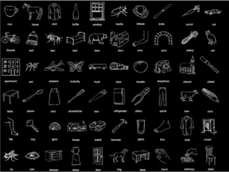
Nine right-handed human participants were scanned in this study. They answered 20 questions (e.g. Was it ever alive?, Can you pick it up?) about 60 different concrete objects equally divided into 12 categories (tools, foods, animals, etc…). Each object was represented by a line drawing and corresponding written noun below it (the complete set of the 60 line drawings can be seen in Appendix A, and the set of 20 questions is shown in Appendix B). Picture and word were positioned as close as possible in order to minimize saccades between the two. A question was presented first, then all 60 nouns were presented in a random order (see Fig. 1). The subjects used a response pad to answer yes or no after each noun presentation. Each stimulus was displayed until one of the buttons was pressed. After answering the question for all 60 nouns, a new question would come up, and the 60 nouns were randomly presented again. This cycle continued for a total of 20 questions. The questions were divided into blocks of 3 questions each (i.e. a question followed by the 60 nouns randomly displayed, then another question, etc), and the subjects had as much time as needed to rest in between blocks (no more than 3 min considering all subjects). Each block lasted approximately 8 min, depending on the subject’s reaction time.

Fig. 1.

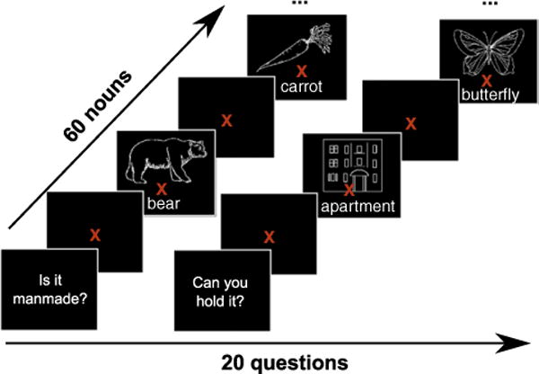
Experimental paradigm. Subjects are first presented with a question, followed by the 60 nouns (combination of picture and word) in a random order. Each stimulus is displayed until the subject presses a button to answer yes or no to the initially presented question. A new question is shown after all 60 nouns have been presented. A fixation point is displayed for 1 s in between nouns and questions.

Computing cluster

The computations described in this paper were performed using the Open Cirrus (Avetisyan et al., 2010) computing cluster at Intel Labs Pittsburgh. The analyses were implemented using the Parallel Computing Toolbox (PCT) of MATLAB® and executed using the virtual machine manager Tashi.

Methods

MEG data preprocessing

The data were preprocessed using the Signal Space Separation method (SSS) (Taulu and Simola, 2006; Taulu et al., 2004). SSS divides the measured MEG data into components originating inside the sensor array vs. outside or very close to it, using the properties of electromagnetic fields and harmonic function expansions. The temporal extension of SSS (tSSS) further enables suppressing components that are highly correlated between the inner and close-by space, such as mouth movement artifacts. Finally, tSSS realigned the head position measured at the beginning of each block to a common location. The MEG signal was then low-pass filtered to 50 Hz to remove the contributions of line noise and down-sampled to 200 Hz. The Signal Space Projection method (SSP) (Uusitalo and Ilmoniemi, 1997) was subsequently applied to remove signal contamination by eye blinks or movements, as well as to remove MEG sensor malfunctions or other artifacts (Vartiainen et al., 2009). Freesurfer software (http://surfer.nmr.mgh.harvard.edu/) was used to construct the 3D model of the brain from the structural MRIs, and to automatically segment, based on each subject’s anatomical data, the 67 regions of interest (ROIs) analyzed in this paper (Freesurfer ‘aparc’ annotation, Desikan–Killiany Atlas). The Minimum Norm Estimates method (Hämäläinen and Ilmoniemi, 1994), which finds the distribution of currents over the cortical mantle that has the minimum overall power, was employed to generate source localized estimates of brain activity from MEG data (MNE Suite software, http://www.nmr.mgh.harvard.edu/martinos/userInfo/data/sofMNE.php).

MNE test sources were evenly distributed (20 mm between neighboring sources, loose orientation constraint of 0.2) in each subject’s cortical sheet, for an average of 1635 sources per subject. A higher number of sources could not be evaluated due to computational costs. Data between −0.1 s and 0.75 s were used in the analysis, where 0 was when the stimulus was presented. Note that while we do not expect that neural activity before stimulus onset contributes to the decoding presented in this paper, utilizing these time points works as a good sanity check for our results (e.g. decoding accuracies in that period should not be better than chance). Source localization was performed separately for each stimulus noun, using the average of 20 MEG trials across the 20 questions.

Training and testing decoders of stimulus features

To study the question of when and where MEG activity encodes various features of the noun stimulus, we used a machine learning approach.

Standard machine learning methods such as support vector machines, logistic regression, and linear regression learn a function f:X → Y, that maps a set of predictive features X to some predicted value Y (Fig. 2, left). For example, the predictive features X might be the observed activity in MEG sensors at some location, averaged over a particular time window, and Y might be a variable indicating whether the subject is reading the stimulus word “house” or “horse”. Alternatively, Y could also be some feature of the stimulus word, such as the number of characters in the word (a perceptual feature) or a variable indicating whether or not the stimulus word describes a living thing (a semantic feature). Whatever the case, the machine learning algorithm creates its estimate $\widehat{f}$ of the function f from a set of training examples consisting of given 〈x,y〉 pairs. The learned $\widehat{f}$ can then be tested by giving it a new example x, and testing whether its prediction $\widehat{f}(x)$ gives the correct value y.

Fig. 2.

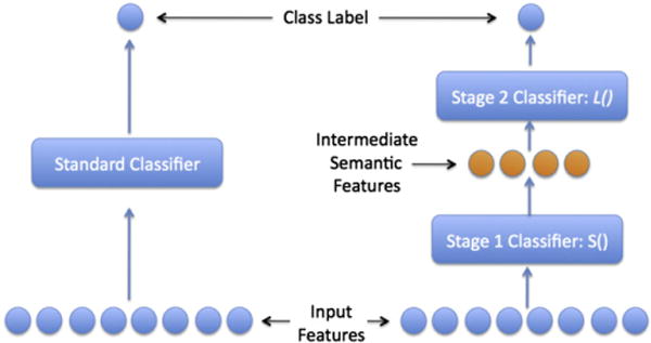
A typical single stage classifier (shown on left) compared to the semantic output code classifier (SOCC, shown on right). The SOCC is a two stage classifier that uses a layer of intermediate semantic features between the input features and the class label. These semantic features represent attributes of the class labels. In our experiments, the input features are the MEG data, the class labels are different nouns (e.g. bear, carrot), and the intermediate semantic features are data collected using Mechanical Turk about the different nouns (e.g. is it alive? can you hold it?).

Here, we use the success or failure of the learned function $\widehat{f}:X\to Y$ in predicting Y over the test data to explore what information is encoded in the MEG activity X. In particular, if $\widehat{f}$ can accurately predict the value y of variable Y for MEG images x, over pairs 〈x,y〉 that were not involved in training $\widehat{f}$, then we conclude that the MEG activity X in fact encodes information about Y. In the analyses reported here, we varied X to cover different spatial regions of source-localized MEG data, and different windows in time, to explore which of these spatial–temporal subsets of MEG activity in fact encode Y. We varied Y to cover hundreds of different semantic and perceptual features. We then tested the accuracy of these trained functions to determine which make accurate predictions, in order to study which of the different spatial–temporal segments of MEG activity X encode which of the different stimulus features Y.

We collected a semantic knowledge base for 1000 concrete nouns using the Mechanical Turk human computation service from Amazon.com https://www.mturk.com/mturk/welcome. Humans were asked 218 questions about the semantic properties of the 1000 nouns, and the 60 nouns presented in the study represent a subset of these nouns. The questions were inspired by the game 20 Questions. For example, some questions were related to size, shape, surface properties, context, and typical usage. These were selected based on conjectures that neural activity for concrete objects is correlated to the sensory and motor properties of the objects (Martin and Chao, 2001). Example questions include is it shiny? and can you hold it? (the complete list of semantic and perceptual features used can be seen in Appendix C). Users of the Mechanical Turk service answered these questions for each noun on a scale of 1 to 5 (definitely not to definitely yes). At least three humans scored each question and the median score was used in the final dataset. For some of the analyses, the set of 218 semantic features was complemented by 11 perceptual features, such as word length and number of white pixels.

In addition to training individual functions to determine which features are encoded where and when in the MEG signal, we also considered the question of whether the features that were decodable by our functions were, in fact, decoded accurately enough to distinguish individual words from one another based on their decoded feature values. This test gives a crude measure of whether our approach captures the majority of the features represented by neural activity (sufficient to distinguish arbitrary pairs of words) or just a fraction of these features. To accomplish this, we trained all decoders for the 218 semantic features, then applied them to decode the features of a novel stimulus word (not included in the training set). To test the accuracy of this collection of decoded features, we asked the predictor which of two novel stimulus words the subject was viewing when the test MEG image was captured, based on its collection of predicted features. We call this two-stage classifier the semantic output code classifier (SOCC, Fig. 2, right), which was first introduced by Palatucci et al. (2009).

Regression model and SOCC

We used a multiple output linear regression to estimate $\widehat{f}$ between the MEG data X and the set of perceptual and semantic features Y (Fig. 2, right). Each semantic or perceptual feature was normalized over the different nouns, such that the final vector of values for each feature used in the regression had a mean of 0 and variance of 1. A similar normalization process was applied to the MEG data, namely, the activity of a source at a given timepoint (i.e. a feature in the regression) was normalized such that its mean over the different observations of the data was 0, and the variance was 1. Let X∈ℜ^N*^d be a training set of examples from MEG data where N is the number of distinct noun stimuli. Each row of X is the average of several repetitions of a particular noun (i.e. for this experiment, the average of several sources over time over the 20 repetitions of a given noun) and d is the number of dimensions of the neural activity pattern. Let F∈ℜ^N*^P be a matrix of p semantic features for those N nouns. We learn a matrix of weights $\widehat{\mathbf{W}}\in {\Re }^{d\ast p}$ which maps from the d-dimensional neural activity to the p semantic features. In this model, each output is treated independently, so we can solve all of them quickly in one matrix operation:

$$\widehat{\mathbf{W}}={({\mathbf{X}}^T\mathbf{X}+\lambda {\mathbf{I}}_{\mathbf{d}})}^{-1}{\mathbf{X}}^T\mathbf{F}$$ (1)

where I_d is the identity matrix with dimension d*d and λ is a scalar regularization parameter chosen automatically using the cross-validation scoring function (Hastie et al., 2011, page 216).¹ A different λ is chosen for each output feature in Y. One disadvantage of Eq. (1) is that it requires an inversion of a d by d matrix, which is computationally slow (or even intractable) for any moderate number of input features. With this form, it would be impossible to compute the model for several thousands of features without first reducing their number using some method of feature selection.

However, a simple computational technique can overcome this problem by rewriting Eq. (1) in its dual form, also known as its kernel form. Following the procedure described in Jordan and Latham (2004) we obtain:

$$\widehat{\mathbf{W}}={\mathbf{X}}^T{(\mathbf{X}{\mathbf{X}}^T+\mathrm{\lambda }{\mathbf{I}}_N)}^{-1}\mathbf{F}$$ (2)

This equation is known as kernel ridge regression and only requires inversion of an N*N matrix. This is highly useful for neural imaging tasks where N is the number of examples which is typically small, while the number of features d can be very large. Another computational technique from Guyon (2005) further shows that with a little pre-computation, it is possible to obtain the inverse for any regularization parameter λ. in time O(N), much faster than the time required for a full inverse O(N³). Combined with the cross-validation scoring function from Hastie et al. (2011, page 216), the end result is an extremely fast method for solving the resulting regression even with thousands of input and semantic features, while automatically selecting the best regularization parameter λ from a large grid of possible parameter choices.²

Using this form, it is possible to quickly obtain the weight matrix $\widehat{\mathbf{W}}$. Then, given a novel neural image x∈ℜ^1*d, we can obtain a prediction $\widehat{\mathbf{f}}\in {\mathcal{R}}^{1\ast p}$ of the semantic features for this image by multiplying the image by the weights:

$$\widehat{\mathbf{f}}=\mathbf{x}\cdot \widehat{\mathbf{W}}$$ (3)

We performed a leave-two-out-cross-validation and trained the model in Eq. (2) to learn the mapping between 58 MEG images and the set of features for their respective nouns. For the second stage of the semantic output code classifier, we applied the learned weight matrix $\widehat{\mathbf{W}}$ to obtain a prediction of the 218 semantic features, and then we used a Euclidean distance metric to compare the vector of predictions to the true feature encodings of the two held-out nouns (Palatucci et al., 2009). The labels were chosen by computing the combined distance of the two labeling configurations (i.e. the nouns with their true labels or the reverse labeling) and choosing the labeling that results in the smallest total distance (Mitchell et al., 2008). For example, if dist() is the Euclidean distance, and p₁ and p₂ are the two predictions for the held out nouns, and s₁ and s₂ are the true feature encodings, then the labeling was correct if:

$$\mathit{dist}(p_1,s_1)+\mathit{dist}(p_2,s_2)<\mathit{dist}(p_1,s_2)+\mathit{dist}(p_2,s_1)$$

This process was repeated for all $\left(\begin{array}{c}60\\ 2\end{array}\right)=1770$ possible leave-two-out combinations.

Because the experimental task involved a button press in every trial, we were also careful not to extend the decoding period past 0.75 s to avoid the contributions of cortical activity associated with the button press (group-level mean reaction time 1.1 s) (Cheyne et al., 2006). As a further confirmation that the information contained in the button presses was not contributing to our decoding results, we ran our classifier for each subject with a single feature as the input, representing the button press value (yes or no), replacing the brain data previously used. Similarly to what was done to the brain data, the feature representing the button press was averaged over all 20 repetitions of a noun. The accuracy of the classifier was not better than chance (50%). We also performed a similar test by using only the EOG signal of each subject as the input to the SOCC. The decoding results were again not better than chance for any of the subjects, suggesting that any remaining eye movement artifacts possibly captured by the EOG channels did not contribute to the decoding results shown in this paper.

Feature scoring

In order to quantify how well each of the semantic features was predicted in the first stage of the SOCC, Eq. (4) was used:

$${\mathit{score}}_{\mathit{feature}}=1-\frac{{\displaystyle \sum {\left(f_i-{\widehat{f}}_i\right)}^2}}{{\displaystyle \sum {\left(f_i-\overline{f}\right)}^2}}$$ (4)

where f_i is the true value of the semantic feature for noun i held-out from the training set in the cross validation, $\overline{f}$ is the mean true feature value over all nouns, ${\widehat{f}}_i$ is the predicted value of the semantic feature for the held-out noun i, and the summation is over all cross-validation iterations. Eq. (4) is a measure of the percent of variance in the feature that is explained by our learned function. So, the closer the semantic feature score is to 1, the better it is predicted by our classifier using MEG data. Eq. (4) is also known in the literature as the coefficient of determination (R²) (Steel and Torrie, 1960).

Statistical significance

Statistical significance was established by running the computational analysis several times with permuted data. More specifically, in each permutation set one subject was chosen at random according to a uniform distribution, and the trial labels for that subject were shuffled prior to averaging over the 20 repetitions. The computational analysis, including source localized estimates, was conducted with the shuffled data set. These analyses were performed over three hundred times, and the results were combined to form null distributions. Finally, the p-values of the reported results were obtained for each individual subject by using a normal kernel density function to estimate the cumulative distribution associated with the empirical null distributions. p-Values across subjects were combined using Fisher’s method (Fisher, 1925), and correction for multiple comparisons (over time, features, and/or regions; indicated in the pertinent parts of the results section) was done using False Discovery Rate (Benjamini, 2001) with no dependency assumptions, at an alpha level of 0.01.

Results

Prior to using the methods described above, an initial analysis of the data revealed that the cortical dynamics generated in this paradigm matched what has been shown in the literature to occur while subjects view pictures or words (Salmelin, 2007). These results made us comfortable to carry out an analysis to address the following questions.

Can we discriminate between two novel nouns only using semantic features predicted from MEG activity?

The input of the classifier consisted of all estimated sources and their activity over time, and only the 218 semantic features were predicted using the data in the first stage of the SOCC. Based on the results shown in Table 1, we see that, for each of the nine participants, it was possible to discriminate with better than 85% accuracy (mean accuracy 91%) between two nouns based on semantic features predicted from observed MEG activity, even though neither noun appeared in the training set.

Table 1.

Accuracies for the leave-two-out experiment using simultaneously all time points from stimulus onset to .75 s and all sources in the cortex as input features for the classifier. The classifiers are able to distinguish between two different concrete nouns that the MEG-based classifier has never seen before with 91% mean accuracy over the nine participants S1 through S9. Chance accuracy was 50.0%. For a single-subject model, 62.5% correspond to p<10⁻² and 85.25%, the result for the subject with the lowest accuracy, to p<10⁻⁶. The p value associated with observing that all nine independently trained participant models exhibit accuracies greater than 62.5% is p<10⁻¹¹.

	S1	S2	S3	S4	S5	S6	S7	S8	S9	Mean
Leave-two-out accuracy	88.25	95.82	86.16	95.20	93.62	92.49	92.54	85.25	91.36	91.19

We also evaluated the decoding accuracy over time by training distinct functions to decode each of the 218 semantic features using consecutive 50-ms time windows of MEG data. The black solid lines in the bottom plots of Fig. 3 show that, when distinguishing between two left-out nouns using all regions of the cortex, the accuracies started to exceed the chance level at 50–100 ms. The peak accuracy was reached at 350–400 ms.

Fig. 3.

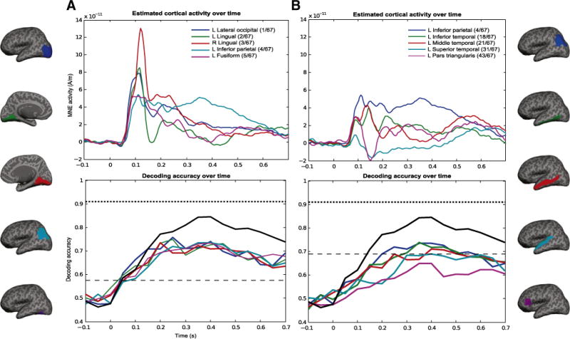
Time courses of activity (top) and decoding accuracy (bottom) in different brain areas. (A) Five ROIs with best decoding results, (B) ROIs pre-selected based on fMRI literature (Price, 2010). The ROIs used in the analysis are displayed on an inflated brain. In each column, top plots denote time courses of activation in the ROIs and bottom plots corresponding time courses of decoding accuracy. Estimated MEG activity for all sources in the different ROIs (different traces in the plot), was averaged over all 60 nouns and across subjects. Decoding accuracy over time was averaged over all subjects. There are clear differences between the time course of MEG activity and that of decodable semantic information. Each time window is 50-ms wide, taken at steps of 50 ms, starting at −0.1 s. For example, the time point at 0.3 s in the bottom graphs shows the decoding accuracy for the window 300–350 ms. Time zero indicates stimulus onset. Chance accuracy is 50%, and light dashed line shows the accuracy above which all values are significant for the different ROIs and time points (p<.01, FDR corrected for multiple comparisons over time and all ROIs). Darker dashed line denotes the mean accuracy over all subjects when the classifier is allowed to observe all time points and sources (i.e. no averages within time windows, same as Table 1). Black solid line indicates decoding accuracy over time when all sources on the cortex were used for each 50-ms time window. Legends in the top row also indicate the rank order of the ROI out of the 67 possible ROIs.

How do the prediction results vary over time and space?

The relatively high temporal and spatial resolution of MEG allows us to address the question of what regions of the brain and at what time points are responsible for these results. For this computational experiment, only the Freesurfer-based pre-specified ROIs were used, and all non-overlapping 50 ms time windows between −0.1 s and 0.75 s were considered.

The activity and decoding accuracy curves of the 5 regions that showed best decoding accuracy over all subjects are displayed in Fig. 3A. The different regions were ranked based on how many significant time points they showed. Then, in the situations when there was a tie in the number of significant accuracies over time, the ROIs in the tie were sorted by maximal decoding accuracy. Most ROIs (63 out of 67) had at least one time point with significant decoding accuracy, and for the top 2 ROIs all windows starting at 50 ms after stimulus onset displayed significant decoding accuracies. In the next best 14 ROIs, all windows starting at 100 ms showed significant decoding accuracies. The complete rank of ROIs can be found in the supplemental website (http://www.cs.cmu.edu/afs/cs/project/theo-73/www/neuroimage2012.html).

Using all sources and time points together resulted in even better decoding accuracies (dashed horizontal black line in Fig. 3, bottom). Using all sources over 50 ms time windows also produced higher decoding accuracy than just using individual ROIs, especially after 200 ms (see difference between black solid curve and other curves). Another way to look at the evolution of the activity and decodability over time is to plot such curves for regions described in fMRI literature to participate in semantic processing (Price, 2010), as seen in Fig. 3B. We selected seven ROIs: left pars opercularis, pars orbitalis, pars triangularis, inferior, middle, and superior temporal cortices, and inferior parietal cortex. One of these regions (left inferior-parietal cortex) was among the top ROIs for decoding, with significant accuracies in all windows from 50 to 700 ms, but the other regions did not rank as well (see legend of the top plots). It is not necessarily surprising that these pre-selected ROIs would not perform as well as the regions shown in Fig. 3A, and also not rank high among all regions that were analyzed, since regions active in fMRI may not fully correspond to the MEG activations (Nunez and Silberstein, 2000).

Note that the time course of activity (top plots in Fig. 3) does not coincide with the evolution of decoding accuracy for the majority of the regions plotted. For example, although activity in left lateral occipital cortex peaks at around 115 ms, its peak decoding happens in the window 200–250 ms. It is also interesting to note the gap between decoding over time that includes all sources and decoding within each individual ROI (i.e. solid black line versus colored lines in the bottom plots of Fig. 3). As none of the single regions reached the decoding accuracy indicated by the solid black line, one can infer that the combination of the activity of several regions markedly contributes to processing of semantic information.

What features are best predicted?

It is also interesting to take a step back and look at the semantic features that were best predicted by the first stage of the classifier (Table 2). When the activity in all sources and time points was used simultaneously as the input to the SOCC (e.g. results in Table 1), a single feature score could be calculated for each semantic feature (Eq. (4)). Out of the 218 semantic features, 184 were predicted with statistically significant accuracy by our method (p<0.01, FDR corrected for multiple comparisons across features). The larger the number of semantic features that were significantly predicted for a subject, the better was the accuracy for that subject in distinguishing between the two left-out nouns. Table 2 shows the top 20 features based on their mean feature score across subjects. It is possible to see a pattern across the well-predicted features. They group around three general categories: size (is it bigger than a car? is it bigger than a loaf of bread?), manipulability (can you hold it? can you pick it up?), and animacy (is it man-made? is it alive?). The complete list of decodable features can be found in the accompanying website (http://www.cs.cmu.edu/afs/cs/project/theo-73/www/neuroimage2012.html).

Table 2.

Top 20 semantic features sorted by mean feature score when using data from all time points and sources in the cortex (p<0.01, FDR corrected for multiple comparisons over features). Features related to size, manipulability, and animacy are among the top semantic features predicted from MEG data.

Mean score (±SD)	Semantic feature
0.59 (±0.07)	Can you pick it up?
0.57 (±0.08)	Is it taller than a person?
0.57 (±0.04)	Is it alive?
0.57 (±0.08)	Is it bigger than a car?
0.57 (±0.08)	Can you hold it?
0.56 (±0.04)	Is it manmade?
0.56 (±0.08)	Can you hold it in one hand?
0.56 (±0.09)	Is it bigger than a loaf of bread?
0.55 (±0.06)	Is it bigger than a microwave oven?
0.55 (±0.06)	Is it manufactured?
0.55 (±0.06)	Is it bigger than a bed?
0.54 (±0.05)	Does it grow?
0.54 (±0.06)	Is it an animal?
0.54 (±0.05)	Was it ever alive?
0.53 (±0.08)	Does it have feelings?
0.53 (±0.04)	Can it bend?
0.53 (±0.08)	Can it be easily moved?
0.53 (±0.06)	Is it hairy?
0.51 (±0.06)	Was it invented?
0.51 (±0.04)	Does it have corners?

To better illustrate the inner workings of the algorithm to distinguish between two nouns, we may analyze the prediction results for a few of the best predicted features and pairs of representative nouns (Fig. 4). Although the predictions are not perfect, they provide a good estimate of the semantic features for the selected nouns. Even when the predicted value does not agree with the target value, that information is still useful to the second phase of the classifier because of the comparative score that was used. For example, although a small positive value was predicted for a screwdriver being bigger than a car, which is obviously not true, that value was nevertheless closer to the true feature value of screwdriver than church, and thus useful for classification. However, the pair key and tomato is not properly classified over the subjects. From Fig. 4, we can see that the target values for those semantic features for the two nouns are very similar, and although they are reasonably well-predicted, it is not enough to differentiate between the two nouns.

Fig. 4.

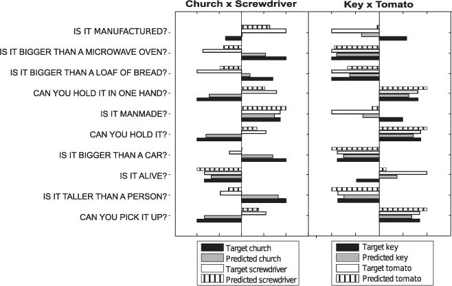
Illustrative example showing predictions for the 10 most predictable semantic features (Table 2) for subject S5, for two representative pairs of nouns (i.e. the two nouns that were left out of the training set). The SOCC performs well even when all features are not predicted correctly. Target denotes the actual semantic feature value for the noun, and the predicted one is the result of the classifier. For this figure, the feature values were normalized to the maximum absolute value per feature (i.e. the longest bar in each feature shares the same absolute value, and the other bars were scaled relative to that).

When and where are perceptual and semantic features predicted in time?

Analyzing how decodable each type of feature is over time also yields interesting insights (Fig. 5). For the following computational experiments, 11 perceptual features were added to the set of 218 semantic features, and we probed when during the response each feature could be reliably decoded. Across subjects, we see that perceptual features such as word length and right-diagonalness have high scores across subjects during the early processing of the stimuli (starting at 50 ms). Later during the course of the response, the score for semantic features starts to rise, while the score for perceptual features drops.

Fig. 5.

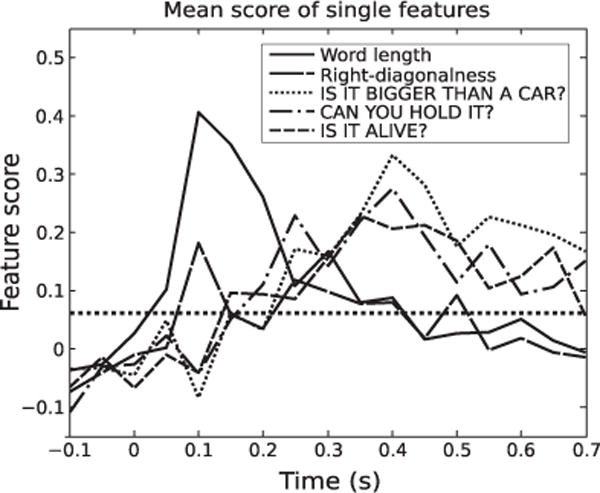
Evolution of the mean feature score for five representative features. Perceptual features such as word length are decoded from MEG data earlier than semantic features. Mean score was taken over feature scores for all subjects using all cortical data. Perceptual features were the two best predicted among subjects. Semantic features were taken from Table 2 and represent 3 distinct groups of features (size, manipulability, and animacy). Black dotted line shows the score above which all scores in the plot become significant (p<10⁻³, FDR corrected for comparisons over features and time).

The feature word length was the best decoded perceptual feature. This might be because the majority of subjects reported upon completion of the experiment that the word was the first part of the stimuli to which they actively attended, and the picture was attended to later (if at all). Still, we can see from the plot the second-best decoded perceptual feature, right diagonalness, also showed an early rise around 50–100 ms, earlier than the semantic features.

It is also interesting to check which regions of the cortex are the source of MEG signal that encodes different features. Fig. 6 shows the top three features decoded from MEG data of different regions of the cortex. Only the sources within each ROI were used to predict both semantic and perceptual features over time (50-ms non-overlapping windows) in the first stage of the SOCC. The ROIs displayed in Fig. 6 are composed of the ROIs that yielded best decoding accuracy (see Fig. 3) and pre-selected regions based on literature (Price, 2010).

Fig. 6.

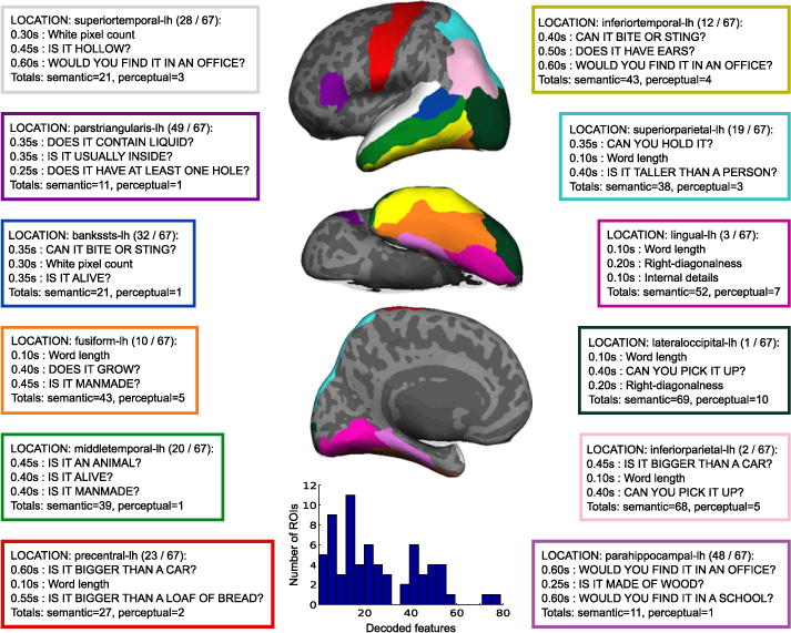
Spatio-temporal characterization of feature decodability in the brain. Perceptual features were better decoded earlier in time using MEG data from posterior regions in the cortex, and semantic features later in time from data of more anterior and lateral regions. Each table shows the three most accurately decoded features for a given ROI, where the color of the table border matches the region marked in the brain plots. Features within a ROI were ranked based on the median peak score over 9 subjects. A row in the table also shows the median time point when that feature reached its peak score (medians taken over 9 subjects). All features shown were significantly predicted with p<10⁻⁵ (corrected for multiple comparisons over features, regions, and time). Each table also shows the ROI rank in predicting features (based on how many features the ROI significantly decoded), and the total number of semantic and perceptual features that were significantly decoded using data from that region. Inflated brain plots display the different ROIs in three different views of the left brain hemisphere: lateral (top), ventral (center, where right is occipital cortex and left is frontal cortex), and medial (bottom). Inset shows a histogram of the total number of features encoded in the 67 ROIs.

The different ROIs were also ranked based on how many features they significantly encoded. Then, in situations when there was a tie in the number of significant features, the ROIs in the tie were sorted by the number of semantic features they encoded. All 67 ROIs encoded at least one feature. Only two regions encoded more than 60 of the 229 features: left lateral occipital and left inferior parietal regions. The histogram in the inset of Fig. 6 summarizes the number of decoded features per ROI. The supplemental website contains a list of the most accurately decoded features for each ROI investigated (http://www.cs.cmu.edu/afs/cs/project/theo-73/www/neuroimage2012.html).

As one might expect, low-level visual properties of the stimuli, such as word length, were best predicted from the neural data in the lateral-occipital cortex around 150 ms. In fact, across regions all perceptual features were usually decoded before 250 ms, with the majority of them decoded at 100–200 ms. Another region that showed preference for decoding perceptual features is the left lingual gyrus, for which all top 3 features were perceptual. Here again, word length was the best predicted feature, with the other perceptual features following close behind.

In most regions the semantic features were predictable from neural data beginning around 250 ms, with a peak in the window at 400–450 ms when considering all regions. There was a clear evolution of the peak time window when the top semantic features were decoded. More specifically, the peak decoding window for semantic features occurred earlier (around 300–400 ms) in posterior regions such as the banks of the superior temporal sulci or the inferior parietal gyrus than in the more anterior regions, such as the precentral cortex and left pars opercularis. Finally, we were interested in whether specific cortical regions were associated with specific semantic feature types. For example, can we predict features related to manipulability better in the precentral region? Features such as can you hold it? and can you hold it in one hand? were among the top 6 decoded features in that region (out of 27 significantly decoded semantic features, p<10⁻⁵ FDR corrected for multiple comparisons over features, time, and space). Another region showing such specificity was the parahippocampal gyrus in the left hemisphere. Features related to a specific location, such as would you find it in an office?, would you find it in a house?, and would you find it in a school? were ranked among the top 6 decoded features using data from that region (out of 11 significantly predicted semantic features, p<10⁻⁵ FDR corrected for multiple comparisons over features, time, and space).

Discussion

We have shown in this paper a methodological approach based on machine learning methods that can be used to identify where and when the MEG signal collected during stimulus comprehension encodes hundreds of semantic and perceptual features. Applying this analysis we found that semantic features related to animacy, manipulability, and size were consistently decoded across subjects. These semantic features were encoded in later time windows, after 250 ms, than perceptual features related to the visual stimuli, which were best decoded before 200 ms. Finally, we have shown that MEG activity localized to certain regions of the brain, such as the lateral occipital cortex and the lingual region, was preferentially related to encoding perceptual features, whereas activity localized to other brain areas, such as the inferior parietal and inferior temporal regions, showed preference for encoding semantic features.

We have also shown that our algorithms can decode a diverse set of semantic features with sufficient accuracy that these decoded semantic features can be used to successfully distinguish which of two words the subject is considering. We report 91% accuracy in distinguishing between pairs of stimulus words based on semantic features decoded from MEG data, even when neither word was present in the training data. When this decoding task was performed using different 50 ms windows in time, the best decoding time window turned out to be from 250 to 450 ms post stimulus onset. This time frame of decoding further supports the hypothesis that the classifier uses semantic information for classification, as several studies have demonstrated the importance of this time window for semantic processing (Kutas and Federmeier, 2000; Salmelin, 2007; Vartiainen et al., 2009; Witzel et al., 2007); purely perceptual characteristics of the stimuli influence cortical activity earlier. We also found that the time course of MEG activity and the time course of decoding accuracy based on semantic features did not coincide, suggesting that only a fraction of the total MEG activity is involved in encoding stimulus semantics. The present results also support the notion that different decoding accuracies at different time windows are not simply a result of higher signal-to-noise ratio in the MEG data, the peak of which should presumably occur at the peak of MEG activity.

This dissociation between the time at which the MEG activity peaks and the time at which the information about semantic features peaks highlights the importance of using a novel data analysis method like ours, that decodes specific information from MEG signals, in contrast to more standard approaches that merely focus on differences in the magnitude of this activity. The current method is also novel because it uses an intermediate feature set to predict attributes of nouns on which the classifier was never trained. Combined with MEG, this approach allows experimenters to test the relationship of different sets of semantic and perceptual features to brain data, and also to analyze when and where different features are best encoded in the MEG-derived brain activity. Additionally, this method uses cross-validation to test several hypotheses about how perceptual and semantic features are encoded in brain activity. Examples of such hypotheses are the degree of distribution of information encoding, the type of features encoded in the neural signal, the time points that contain most semantic information, the order in which perceptual and semantic features are encoded, etc. In this paper, we showed that such hypotheses can be tested with highly significant results.

While this paper describes an innovative method for tracking the flow of decodable information during language comprehension, the cognitive implications of the results are necessarily limited by the paradigm used while collecting the MEG data. Here, the choice for double stimulation (word and line drawing) was influenced by the group’s previous successful results with a similar paradigm in fMRI (Mitchell et al., 2008; Shinkareva et al., 2008). This set of stimuli was exported to MEG without major modifications, with the primary intent to evaluate the methodological approach described in this paper. One advantage of the present stimulus set is that the line drawings help to disambiguate the word meanings. However, the processing of the word-drawing pair by the subject is likely to include neural subprocesses that would not be present using either picture or word stimuli alone. For example, some of the neural activity we observe might reflect post-perceptual processes of matching the word and the line drawing. It can also be the case that the order in which subjects viewed the word and the picture affects the differences in latencies between the predicted perceptual and semantic features. Additionally, there was a considerable correlation between perceptual and semantic features, and also within the semantic feature set. This correlation is a plausible explanation for the early rise of accuracies even when only semantic features were predicted from the MEG data (Fig. 3). It is our future goal to apply a similar analysis approach to paradigms that avoid the confounds of the double stimulus and are better optimized for the high temporal sensitivity of MEG (Vartiainen et al., 2009). Such paradigms would allow us to study these timing issues directly, better disambiguate between the different perceptual and semantic features, and would also align better with existing studies of the neural correlates of language processing (Hauk et al., 2009).

There is an on-going debate in the language literature about serial versus parallel models of language comprehension (see Pulvermuller et al. (2009) for a review). Proponents of the parallel model cite evidence for early (<250 ms after stimulus onset) manifestations of processing of semantic information (Hauk and Pulvermüller, 2004; Moscoso del Prado Martín et al., 2006). Here, most of the semantic features were encoded later in the trial. While this observation may seem to disagree with the parallel model hypothesis, our two-stimulus protocol was probably not ideal for asking this question, nor was it designed for this specific purpose. These issues will need to be addressed in more detail by future studies that use more optimally designed stimuli and experimental protocols.

The analyses here were based on a set of 218 semantic features, chosen to span a broad space of semantics for concrete noun stimuli. One eventual goal of our research is to identify the key semantic subcomponents, or factors, that are combined by the brain to form neural encodings of concrete word meanings. Our present experimental results show that the 218 semantic features did indeed span a sufficiently diverse semantic space to capture subtle distinctions among our concrete noun stimuli: our approach was able to distinguish which of two novel words was being considered with highly significant accuracy when using only the decoded estimates of these 218 features. The high performance of the model suggests that the stimuli studied here may share a fairly similar grouping in brain signal space and the semantic features space spanned by the 218 features. Furthermore, our results suggest that only a fraction of the 218 features need to be accurately predicted in order to reliably distinguish between the two left-out nouns. The most decodable of the 218 semantic features could be grouped into three main classes: features about animacy, manipulability, and size. These groups are very similar to the 3 factors (shelter, manipulability, eating) previously shown to be relevant to the representation of concrete nouns in the brain (Just et al., 2010), even though that work was done using fMRI, and employed a completely different type of analysis and task performed by the subjects. The other factor singled out by Just et al. (2010), word length, was also consistently predicted in this paper. Moreover, several other studies have shown the importance of animacy in the neural representation of concrete nouns (Lambon Ralph et al., 2007; Mahon and Caramazza, 2009; Moss et al., 2005). In the future, we plan to narrow down the number and type of semantic features being predicted in order to fully characterize a minimal semantic space that is sufficient to obtain comparable results. This will be done by applying dimensionality reduction algorithms to our set of 218 semantic features, as well as to other sets of features such as word co-occurrences, and then interpreting the minimum number of uncorrelated features that are needed to obtain significant accuracies. Also, experiments that use a larger and specially-chosen set of stimuli will help to decrease the between-feature correlation that affects the current results.

One consideration that is fundamental to our research is how to define the difference between perceptual and semantic features. For example, consider the question of whether to define the feature does it have 4 legs? as perceptual or semantic. Of course the dividing line between the two is a matter of definition. We find it useful to adopt the following operational definition: any feature of a concrete noun that a person considers regardless of stimulus modality (e.g. independent of whether the stimulus item is presented as a written noun, spoken noun, or picture) we define to be a semantic feature for that person. Clearly, this definition allows some sensory features such as the shape of a pine tree or the sound of a bell to potentially be semantic features, to the degree that we think of those sensory features automatically when we read the word. Given previous work suggesting that neural representations of concrete noun meanings are largely grounded in sensory–motor cortical regions (Just et al., 2010), this seems appropriate. To the degree that we think of a bell’s sound when reading the word bell, then it seems appropriate to consider it part of the word’s semantics – a part that is also activated directly when we hear the bell instead of read about it. It is also hard to prove, with the current paradigm, that some of the semantic features we decoded here are not simply a correlate of perceptual features that we did not include in our original set. While it would not be possible to list all possible perceptual features for decoding, increasing the variety of features in the set can help with this issue, as well as employing a broader and better-designed set of stimuli that would control for most of these correlations between semantic and perceptual features.

Previous reports that used fMRI data to decode cognitive states showed regions of the brain contributing to decoding results that were not found in this study. For example, parts of the brain that are commonly associated with semantic processing in the fMRI literature (Price, 2010), such as the left pars opercularis and pars orbitalis, did not show high decoding accuracies over time in our MEG study. Regardless of the complications of capturing MEG signatures from different parts of the brain (e.g. from subcortical structures (Hämäläinen et al., 1993)), there are two important points to be made. First, it is common for subjects in fMRI experiments to have a significant amount of time to think about the different properties of an object. Although this time is necessary in order to capture the slowly-rising BOLD response, that also gives the subject the opportunity to think of specific properties of a noun that will involve those regions of the brain. For example, while it is debatable that the distributed representation of a screwdriver involves motor cortex every time the subject thinks of it, if the subject is asked and given enough time to imagine certain properties of a screwdriver, and to do this as consistently as possible across repetitions of screwdriver, it is very likely that holding a screwdriver will come to mind in every repetition, and this way motor cortex will be active (Shinkareva et al., 2008). In our MEG experiments, subjects spent only about 1 s on average considering the noun stimulus. Thus, the MEG signals on which our analysis was based reflect the automatic brain responses when the subjects think briefly of one of the nouns. Another aspect of the fMRI signal that can affect the analysis regards the inherent averaging of signals over time. For example, if the subject thinks of picking an apple and then eating it in one trial, and thinks of the same properties in the opposite sequence in another trial, the resulting image will likely be similar in fMRI, but not MEG. Moreover, because our analysis was conducted on data averaged across trials, the chances of activity that is not time-locked to the stimulus to be washed away in the averaging process are high. It has also been conjectured that MEG gives stronger emphasis to bottom-up processes, while fMRI tends to emphasize more top-down processes (Vartiainen et al., 2011), which would likely be elicited in the longer trials of fMRI experiments and contribute to activation in areas not seen in MEG.

To summarize, we showed that several semantic features can be decoded from the evoked responses in MEG. Nevertheless, it is likely that the responses resembling what is usually seen in fMRI (assuming an unlikely 1–1 correspondence between MEG and fMRI activity), were either not activated by the paradigms, or were offset in time and were not represented in the averages over trials. Regions pre-selected from the fMRI literature did not perform as well as other regions in the cortex in distinguishing which of two novel nouns was being presented. It is clear that the tasks used in fMRI and MEG, as well as the nature of the signals being measured, influence the regions activated in the brain and the results we obtained in the different experiments. The context in which the nouns are thought of can also help to justify some of the results obtained in this paper. On the other hand, we saw some intriguing results regarding certain regions of the cortex displaying a bias towards decoding specific types of features. For example, some of the top semantic features decoded from motor cortex were related to manipulability (e.g. can you hold it?), and the top features predicted from the parahippocampal region were associated with a location (e.g. would you find it in an office?). It is common to see motor cortex involved in the representation of tools, and the parahippocampal region associated with shelter-like features (Just et al., 2010; Mitchell et al., 2008). We hope that future results using this method to analyze the data of better-designed paradigms will help elucidate the role of such regions in decoding these features.

Throughout this paper, we used the concept of encoding/decoding features with the idea that the MEG activity encodes a feature (at least relative to our stimuli) if the algorithms can decode that feature from observed MEG data of a subject processing a novel stimulus. It does not necessarily follow that the brain is using that information to encode the object in question, because the information we are decoding could represent some correlate of the processing the brain performs in such tasks. The results shown in this work also rely on the assumption that perceptual and semantic features are coded by the magnitude of the MEG signal, but there may also be relevant information in other attributes of the signal. Several other types of attributes, such as the power and phase of different frequency bands, or different functional connectivity measures (Kujala et al., 2008), might work as well, if not better, in decoding features, and it is possible that some combination of these different attributes would be the best approach. Another pitfall of using the amplitude of the MEG signals, and averaging them over different trials is the temporal alignment of the features being decoded. One could argue that the problem is ameliorated because we average different repetitions of the same noun, but it is still unlikely that the subjects would think about a given noun with strictly consistent timing across the 20 repetitions. The signal used for feature decoding might thus be washed out by averaging across the repetitions. In fact, that is true for any cognitive processing that is not time-locked to the stimuli. Finally, the way minimum-norm source estimation was used combines the amount of activity within a cortical area to a single unsigned value per time point that represents the total amount of activity for the source at that instant. However, it carries no information about the direction of current flow that can be a functionally highly relevant parameter and might well be helpful in predicting the different perceptual and semantic features used in the analysis. Despite these difficulties, we showed that it is possible to classify several of these features significantly better than chance. These results should only improve when time-invariant attributes are used for decoding, or when different signal processing techniques are applied to make better use of the single trials of MEG data, alleviating the need for using data averaged across multiple trials.

We presented a method that can estimate where and when different perceptual and semantic features are encoded in the MEG activity, but it remains unclear how the information is transformed by the brain from perceptual to semantic features. More work needs to be done to understand how the transformation takes place between the different levels of representation, and also to investigate how the encoding is actually performed in the brain. An interesting future direction could be to perform correlation analysis between the time series of activation in the various areas identified in this study, as it could provide better understanding of how these regions interact to communicate and encode information.

Conclusion

We have presented an effective method for studying the temporal sequence and cortical locations of perceptual and semantic features encoded by observed MEG neural activity, while subjects perceive concrete objects stimuli. The experiments showed intriguing results (albeit limited by the choice of experimental paradigm), and thus encourage further, more carefully controlled and cognitively relevant studies. The current results provide insights about the flow of information encoded by the MEG signal associated with processing of concrete nouns, and revealed discrepancies between regions that show relevant information in MEG and areas previously described in the fMRI literature. Whereas classifiers trained using fMRI can establish where in the brain neural activity distinguishes between different nouns, our results show when and where MEG data localized to different regions of the cortex encode perceptual or semantic attributes of the nouns. We also demonstrated that it is possible to decode several different perceptual and semantic features, and observed that perceptual attributes were decoded early in the MEG response, while semantic attributes were decoded later.

Appendix A. Set of 60 line drawings

Appendix B. Set of 20 questions

• Is it manmade?

• Is it made of metal?

• Is it hollow?

• Is it hard to catch?

• Does it grow?

• Was it ever alive?

• Could you fit inside it?

• Does it have at least one hole?

• Can you hold it?

• Is it bigger than a loaf of bread?

• Does it live in groups?

• Can it keep you dry?

• Is part of it made of glass?

• Is it bigger than a car?

• Can you hold it in one hand?

• Is it manufactured?

• Is it bigger than a microwave oven?

• Is it alive?

• Does it have feelings?

• Can you pick it up?

Appendix C. List of semantic and perceptual features

Single features

Semantic features

1. Is it an animal?

2. Is it a body part?

3. Is it a building?

4. Is it a building part?

5. Is it clothing?

6. Is it furniture?

7. Is it an insect?

8. Is it a kitchen item?

9. Is it man-made?

10. Is it a tool?

11. Can you eat it?

12. Is it a vehicle?

13. Is it a person?

14. Is it a vegetable/plant?

15. Is it a fruit?

16. Is it made of metal?

17. Is it made of plastic?

18. Is part of it made of glass?

19. Is it made of wood?

20. Is it shiny?

21. Can you see through it?

22. Is it colorful?

23. Does it change color?

24. Is one more than one colored?

25. Is it always the same color(s)?

26. Is it white?

27. Is it red?

28. Is it orange?

29. Is it flesh-colored?

30. Is it yellow?

31. Is it green?

32. Is it blue?

33. Is it silver?

34. Is it brown?

35. Is it black?

36. Is it curved?

37. Is it straight?

38. Is it flat?

39. Does it have a front and a back?

40. Does it have a flat/straight top?

41. Does it have flat/straight sides?

42. Is taller than it is wide/long?

43. Is it long?

44. Is it pointed/sharp?

45. Is it tapered?

46. Is it round?

47. Does it have corners?

48. Is it symmetrical?

49. Is it hairy?

50. Is it fuzzy?

51. Is it clear?

52. Is it smooth?

53. Is it soft?

54. Is it heavy?

55. Is it lightweight?

56. Is it dense?

57. Is it slippery?

58. Can it change shape?

59. Can it bend?

60. Can it stretch?

61. Can it break?

62. Is it fragile?

63. Does it have parts?

64. Does it have moving parts?

65. Does it come in pairs?

66. Does it come in a bunch/pack?

67. Does it live in groups?

68. Is it part of something larger?

69. Does it contain something else?

70. Does it have internal structure?

71. Does it open?

72. Is it hollow?

73. Does it have a hard inside?

74. Does it have a hard outer shell?

75. Does it have at least one hole?

76. Is it alive?

77. Was it ever alive?

78. Is it a specific gender?

79. Is it manufactured?

80. Was it invented?

81. Was it around 100 years ago?

82. Are there many varieties of it?

83. Does it come in different sizes?

84. Does it grow?

85. Is it smaller than a golfball?

86. Is it bigger than a loaf of bread?

87. Is it bigger than a microwave oven?

88. Is it bigger than a bed?

89. Is it bigger than a car?

90. Is it bigger than a house?

91. Is it taller than a person?

92. Does it have a tail?

93. Does it have legs?

94. Does it have four legs?

95. Does it have feet?

96. Does it have paws?

97. Does it have claws?

98. Does it have horns/thorns/spikes?

99. Does it have hooves?

100. Does it have a face?

101. Does it have a backbone?

102. Does it have wings?

103. Does it have ears?

104. Does it have roots?

105. Does it have seeds?

106. Does it have leaves?

107. Does it come from a plant?

108. Does it have feathers?

109. Does it have some sort of nose?

110. Does it have a hard nose/beak?

111. Does it contain liquid?

112. Does it have wires or a cord?

113. Does it have writing on it?

114. Does it have wheels?

115. Does it make a sound?

116. Does it make a nice sound?

117. Does it make sound continuously when active?

118. Is its job to make sounds?

119. Does it roll?

120. Can it run?

121. Is it fast?

122. Can it fly?

123. Can it jump?

124. Can it float?

125. Can it swim?

126. Can it dig?

127. Can it climb trees?

128. Can it cause you pain?

129. Can it bite or sting?

130. Does it stand on two legs?

131. Is it wild?

132. Is it a herbivore?

133. Is it a predator?

134. Is it warm blooded?

135. Is it a mammal?

136. Is it nocturnal?

137. Does it lay eggs?

138. Is it conscious?

139. Does it have feelings?

140. Is it smart?

141. Is it mechanical?

142. Is it electronic?

143. Does it use electricity?

144. Can it keep you dry?

145. Does it provide protection?

146. Does it provide shade?

147. Does it cast a shadow?

148. Do you see it daily?

149. Is it helpful?

150. Do you interact with it?

151. Can you touch it?

152. Would you avoid touching it?

153. Can you hold it?

154. Can you hold it in one hand?

155. Do you hold it to use it?

156. Can you play it?

157. Can you play with it?

158. Can you pet it?

159. Can you use it?

160. Do you use it daily?

161. Can you use it up?

162. Do you use it when cooking?

163. Is it used to carry things?

164. Can you pick it up?

165. Can you control it?

166. Can you sit on it?

167. Can you ride on/in it?

168. Is it used for transportation?

169. Could you fit inside it?

170. Is it used in sports?

171. Do you wear it?

172. Can it be washed?

173. Is it cold?

174. Is it cool?

175. Is it warm?

176. Is it hot?

177. Is it unhealthy?

178. Is it hard to catch?

179. Can you peel it?

180. Can you walk on it?

181. Can you switch it on and off?

182. Can it be easily moved?

183. Do you drink from it?

184. Does it go in your mouth?

185. Is it tasty?

186. Is it used during meals?

187. Does it have a strong smell?

188. Does it smell good?

189. Does it smell bad?

190. Is it usually inside?

191. Is it usually outside?

192. Would you find it on a farm?

193. Would you find it in a school?

194. Would you find it in a zoo?

195. Would you find it in an office?

196. Would you find it in a restaurant?

197. Would you find in the bathroom?

198. Would you find it in a house?

199. Would you find it near a road?

200. Would you find it in a dump/landfill?

201. Would you find it in the forest?

202. Would you find it in a garden?

203. Would you find it in the sky?

204. Do you find it in space?

205. Does it live above ground?

206. Does it get wet?

207. Does it live in water?

208. Can it live out of water?

209. Do you take care of it?

210. Does it make you happy?

211. Do you love it?

212. Would you miss it if it were gone?

213. Is it scary?

214. Is it dangerous?

215. Is it friendly?

216. Is it rare?

217. Can you buy it?

218. Is it valuable?

Perceptual features

1. Word length

2. White pixel count

3. Internal details

4. Verticality

5. Horizontalness

6. Left-diagonalness

7. Right-diagonalness

8. Aspect-ratio: skinny→fat

9. Prickiliness

10. Line curviness

11. 3D curviness

References

- Avetisyan AI, Campbell R, Gupta I, Heath MT, Ko SY, Ganger GR, Kozuch Ma, O’Hallaron D, Kunze M, Kwan TT, Lai K, Lyons M, Milojicic DS, Luke JY. Open Cirrus: A Global Cloud Computing Testbed. IEEE Comput. 2010;43:35–43. [Google Scholar]
- Benjamini Y. The Control of the False Discovery Rate in Multiple Testing Under Dependency. Ann Stat. 2001;29:1165–1188. [Google Scholar]
- Cabeza R, Nyberg L. Imaging cognition II: An empirical review of 275 PET and fMRI studies. J Cogn Neurosci. 2000;12:1–47. doi: 10.1162/08989290051137585. [DOI] [PubMed] [Google Scholar]
- Chan A, Halgren E, Marinkovic K, Cash SS. Decoding word and category-specific spatiotemporal representations from MEG and EEG. NeuroImage. 2010;54:3028–3039. doi: 10.1016/j.neuroimage.2010.10.073. [DOI] [PMC free article] [PubMed] [Google Scholar]
- Cheyne D, Bakhtazad L, Gaetz W. Spatiotemporal mapping of cortical activity accompanying voluntary movements using an event-related beamforming approach. Hum Brain Mapp. 2006;27:213–229. doi: 10.1002/hbm.20178. [DOI] [PMC free article] [PubMed] [Google Scholar]
- Guimaraes MP, Wong DK, Uy ET, Suppes P, Grosenick L. Single-trial classification of MEG recordings. IEEE Trans Biomed Eng. 2007;54:436–443. doi: 10.1109/TBME.2006.888824. [DOI] [PubMed] [Google Scholar]
- Guyon I. Kernel ridge regression. ClopiNet; 2005. (Technical Report 10). Notes on Kernel Ridge Regression. [Google Scholar]
- Hämäläinen MS, Ilmoniemi RJ. Interpreting magnetic fields of the brain: minimum norm estimates. Med Biol Eng Comput. 1994;32:35–42. doi: 10.1007/BF02512476. [DOI] [PubMed] [Google Scholar]
- Hämäläinen MS, Hari R, Ilmoniemi RJ, Knuutila J, Lounasmaa O. Magnetoencephalography – theory, instrumentation, and applications to noninvasive studies of the working human brain. Rev Mod Phys. 1993;65:413–507. [Google Scholar]
- Hastie T, Tibshirani R, Friedman J. The Elements of Statistical Learning. Springer; 2011. [Google Scholar]
- Hauk O, Pulvermüller F. Neurophysiological distinction of action words in the fronto-central cortex. Hum Brain Mapp. 2004;21:191–201. doi: 10.1002/hbm.10157. [DOI] [PMC free article] [PubMed] [Google Scholar]
- Hauk O, Davis MH, Kherif F, Pulvermüller F. Imagery or meaning? Evidence for a semantic origin of category-specific brain activity in metabolic imaging. Eur J Neurosci. 2008;27:1856–1866. doi: 10.1111/j.1460-9568.2008.06143.x. [DOI] [PMC free article] [PubMed] [Google Scholar]
- Hauk O, Pulvermüller F, Ford M, Marslen-Wilson WD, Davis MH. Can I have a quick word? Early electrophysiological manifestations of psycholinguistic processes revealed by event-related regression analysis of the EEG. Biol Psychol. 2009;80:64–74. doi: 10.1016/j.biopsycho.2008.04.015. [DOI] [PubMed] [Google Scholar]
- Jordan M, Latham D. Linear and ridge regression, and kernels. UC Berkeley; 2004. (Technical Report. Lecture Notes: Advanced Topics in Learning and Decision Making). [Google Scholar]
- Just MA, Cherkassky V, Aryal S, Mitchell TM. A neurosemantic theory of concrete noun representation based on the underlying brain codes. PLoS One. 2010;5:e8622. doi: 10.1371/journal.pone.0008622. [DOI] [PMC free article] [PubMed] [Google Scholar]
- Kujala J, Gross J, Salmelin R. Localization of correlated network activity at the cortical level with MEG. NeuroImage. 2008;39:1706–1720. doi: 10.1016/j.neuroimage.2007.10.042. [DOI] [PubMed] [Google Scholar]
- Kutas M, Federmeier K. Electrophysiology reveals semantic memory use in language comprehension. Trends Cogn Sci. 2000;4:463–470. doi: 10.1016/s1364-6613(00)01560-6. [DOI] [PubMed] [Google Scholar]
- Lambon Ralph Ma, Lowe C, Rogers TT. Neural basis of category-specific semantic deficits for living things: evidence from semantic dementia, HSVE and a neural network model. Brain. 2007;130:1127–1137. doi: 10.1093/brain/awm025. [DOI] [PubMed] [Google Scholar]
- Mahon BZ, Caramazza A. Concepts and categories: a cognitive neuropsychological perspective. Annu Rev Psychol. 2009;60:27–51. doi: 10.1146/annurev.psych.60.110707.163532. [DOI] [PMC free article] [PubMed] [Google Scholar]
- Martin A. The representation of object concepts in the brain. Annu Rev Psychol. 2007;58:25–45. doi: 10.1146/annurev.psych.57.102904.190143. [DOI] [PubMed] [Google Scholar]
- Martin A, Chao LL. Semantic memory and the brain: structure and processes. Curr Opin Neurobiol. 2001;11:194–201. doi: 10.1016/s0959-4388(00)00196-3. [DOI] [PubMed] [Google Scholar]
- Mitchell TM, Shinkareva SV, Carlson A, Chang Km, Malave VL, Mason RA, Just MA. Predicting human brain activity associated with the meanings of nouns. Science. 2008;320:1191–1195. doi: 10.1126/science.1152876. [DOI] [PubMed] [Google Scholar]
- Moscoso del Prado Martin F, Hauk O, Pulvermüller F. Category specificity in the processing of color-related and form-related words: an ERP study. NeuroImage. 2006;29:29–37. doi: 10.1016/j.neuroimage.2005.07.055. [DOI] [PubMed] [Google Scholar]
- Moss H, Rodd JM, Stamatakis Ea, Bright P, Tyler LK. Antero-medial temporal cortex supports fine-grained differentiation among objects. Cereb Cortex. 2005;15:616–627. doi: 10.1093/cercor/bhh163. [DOI] [PubMed] [Google Scholar]
- Nunez PL, Silberstein RB. On the relationship of synaptic activity to macroscopic measurements: does co-registration of EEG with fMRI make sense? Brain Topogr. 2000;13:79–96. doi: 10.1023/a:1026683200895. [DOI] [PubMed] [Google Scholar]
- Palatucci M, Pomerleau D, Hinton G, Mitchell TM. Zero-shot learning with semantic output codes. Neural Information Processing Systems. Citeseer. 2009:1410–1418. [Google Scholar]
- Price CJ. The anatomy of language: a review of 100 fMRI studies published in 2009. Ann N Y Acad Sci. 2010;1191:62–88. doi: 10.1111/j.1749-6632.2010.05444.x. [DOI] [PubMed] [Google Scholar]
- Pulvermüller F. Brain reflections of words and their meaning. Trends Cogn Sci. 2001;5:517–524. doi: 10.1016/s1364-6613(00)01803-9. [DOI] [PubMed] [Google Scholar]
- Pulvermüller F, Ilmoniemi RJ, Shtyrov Y. Brain signatures of meaning access in action word recognition. J Cogn Neurosci. 2005;17:884–892. doi: 10.1162/0898929054021111. [DOI] [PubMed] [Google Scholar]
- Pulvermüller F, Shtyrov Y, Hauk O. Understanding in an instant: neurophysiological evidence for mechanistic language circuits in the brain. Brain Lang. 2009;110:81–94. doi: 10.1016/j.bandl.2008.12.001. [DOI] [PMC free article] [PubMed] [Google Scholar]
- Rogers TT, Patterson K, Nestor P. Where you know what you know? The representation of semantic knowledge in the human brain. Nat Rev Neurosci. 2007;8:976–987. doi: 10.1038/nrn2277. [DOI] [PubMed] [Google Scholar]
- Salmelin R. Clinical neurophysiology of language: the MEG approach. Clin Neurophysiol. 2007;118:237–254. doi: 10.1016/j.clinph.2006.07.316. [DOI] [PubMed] [Google Scholar]
- Shinkareva SV, Mason Ra, Malave VL, Wang W, Mitchell TM, Just MA. Using FMRI brain activation to identify cognitive states associated with perception of tools and dwellings. PLoS One. 2008;3:e1394. doi: 10.1371/journal.pone.0001394. [DOI] [PMC free article] [PubMed] [Google Scholar]
- Steel RGD, Torrie JH. Principles and Procedures of Statistics. McGraw-Hill; New York: 1960. [Google Scholar]
- Suppes P, Han B, Epelboim J, Lu Z. Invariance of brain-wave representations of simple visual images and their names. Proc Natl Acad Sci. 1999;96:14658–14663. doi: 10.1073/pnas.96.25.14658. [DOI] [PMC free article] [PubMed] [Google Scholar]
- Taulu S, Kajola M, Simola J. Suppression of interference and artifacts by the Signal Space Separation Method. Brain Topogr. 2004;16:269–275. doi: 10.1023/b:brat.0000032864.93890.f9. [DOI] [PubMed] [Google Scholar]
- Taulu S, Simola J. Spatiotemporal signal space separation method for rejecting nearby interference in MEG measurements. Phys Med Biol. 2006;51:1759–1768. doi: 10.1088/0031-9155/51/7/008. [DOI] [PubMed] [Google Scholar]
- Uusitalo MA, Ilmoniemi RJ. Signal-space projection method for separating MEG or EEG into components. Med Biol Eng Comput. 1997;35:135–140. doi: 10.1007/BF02534144. [DOI] [PubMed] [Google Scholar]
- Vartiainen J, Parviainen T, Salmelin R. Spatiotemporal convergence of semantic processing in reading and speech perception. J Neurosci. 2009;29:9271–9280. doi: 10.1523/JNEUROSCI.5860-08.2009. [DOI] [PMC free article] [PubMed] [Google Scholar]
- Vartiainen J, Liljeström M, Koskinen M, Renvall H, Salmelin R. Functional magnetic resonance imaging blood oxygenation level-dependent signal and magnetoencephalography evoked responses yield different neural functionality in reading. J Neurosci. 2011;31:1048–1058. doi: 10.1523/JNEUROSCI.3113-10.2011. [DOI] [PMC free article] [PubMed] [Google Scholar]
- Witzel T, Dhond RPR, Dale AM, Halgren E. Spatiotemporal cortical dynamics underlying abstract and concrete word reading. Hum Brain Mapp. 2007;28:355–362. doi: 10.1002/hbm.20282. [DOI] [PMC free article] [PubMed] [Google Scholar]
Associated Data
This section collects any data citations, data availability statements, or supplementary materials included in this article.