Abstract
Positron emission tomography data are typically reconstructed with maximum likelihood expectation maximization (MLEM). However, MLEM suffers from positive bias due to the non-negativity constraint. This is particularly problematic for tracer kinetic modeling. Two reconstruction methods with bias reduction properties that do not use strict Poisson optimization are presented and compared to each other, to filtered backprojection (FBP), and to MLEM. The first method is an extension of NEGML, where the Poisson distribution is replaced by a Gaussian distribution for low count data points. The transition point between the Gaussian and the Poisson regime is a parameter of the model. The second method is a simplification of ABML. ABML has a lower and upper bound for the reconstructed image whereas AML has the upper bound set to infinity. AML uses a negative lower bound to obtain bias reduction properties. Different choices of the lower bound are studied. The parameter of both algorithms determines the effectiveness of the bias reduction and should be chosen large enough to ensure bias-free images. This means that both algorithms become more similar to least squares algorithms, which turned out to be necessary to obtain bias-free reconstructions. This comes at the cost of increased variance. Nevertheless, NEGML and AML have lower variance than FBP. Furthermore, randoms handling has a large influence on the bias. Reconstruction with smoothed randoms results in lower bias compared to reconstruction with unsmoothed randoms or randoms precorrected data. However, NEGML and AML yield both bias-free images for large values of their parameter.
Index Terms: Image reconstruction, iterative methods, positron emission tomography (PET)
I. Introduction
Nowadays, positron emission tomography (PET) reconstruction is mainly done by applying iterative reconstruction methods. Iterative reconstruction is based on a forward model, which offers the possibility to model the true acquisition process better than analytical methods, e.g., by incorporation of finite resolution, irregularities in the geometry, etc. Iterative reconstruction in PET is usually based on a maximum likelihood (ML) approach, to take into account the Poisson statistics of the measured data. To suppress the noise propagation, the likelihood can be combined with a prior that favors smooth reconstructions [1].
The most popular iterative ML method for PET reconstruction is ML expectation maximization (MLEM [2], [3]). MLEM reconstructions tend to be biased in regions with low activity, in particular if these regions are surrounded by high activity structures. Moreover, MLEM suffers from noise induced bias [4]. This means that for kinetic PET studies, analytical methods, like filtered backprojection (FBP), are still the method of choice despite the fact that these images have often lower resolution and more streak artifacts due to noise [5], [6]. Dynamic PET data have often very limited numbers of counts that are sparsely divided over the lines of response. This is due to the fact that the early frames are often very short and for late frames only limited activity might be left due to the decay of the activity [6]. When bias is present in the derived time-activity curves, the resulting kinetic rate constants will also be biased. Increased variance is usually less problematic, because its influence is suppressed by fitting the kinetic model to a fairly large number of data points [11].
In every iteration of the MLEM algorithm, the current reconstruction image λ is updated by adding the image Δλ which is given for voxel j by
| (1) |
with
| (2) |
where yi are the measured counts for detector pair i, ŷi is the estimate of the sinogram mean based on the current reconstruction λ, cij is the sensitivity of detector pair i for activity in voxel j, and ri is the estimated number of scattered and/or random events.
The reconstruction formula in (1) shows that the update of a voxel is proportional to λj, the current activity estimate for voxel j. This means that regions with low activity with respect to the rest of the reconstruction, will converge much slower and a very high number of iterations is required to eliminate the positive bias. In practice one is not usually iterating long enough to avoid this incomplete convergence bias. Since there are other causes of bias, iterating longer by itself would not make the image bias-free.
The inherent non-negativity constraint in image space means that creating a region with zero mean is only possibly by making all voxels zero since no negative voxels values are allowed. Under noisy circumstances MLEM will always have some remaining positive bias in low-activity regions. FBP reconstruction has no constraints on the image values and has usually both positive and negative values in a cold region. In case of very noisy data (i.e., with very low counts), MLEM not only introduces bias in cold regions but also in regions with higher activity. It is known that MLEM with Poisson likelihood is only asymptotically unbiased, which means that it is only unbiased for an infinite number of counts [7], [8]. Each realization is forced to be positive and this positivity constraint is the origin of this bias. This property causes, even at convergence, positive bias in the image for low count measurements.
The ABML-method proposed by Byrne in [9] can be used for bias reduction. The ABML method extends MLEM by minimizing the Kullback-Leibler (KL) distance, between yi and ŷi, using a lower boundary A and upper boundary B. It is based on a well chosen combination of KL distances [9] such that when applying the natural constraints of MLEM, A = 0 and B = ∞, minimizing the KL cost function is equivalent to maximizing the Poisson likelihood. By setting A to negative values, negative values in the image and sinogram domain are allowed, resulting in bias reduction behavior [10]–[12]. The convergence of different regions is still dependent on the activity but to a lesser extent. Since reconstruction values are usually not known beforehand, upper bound B is often chosen very high and A is often set to a very low value (i.e., a negative value with high magnitude). It was not evaluated whether less extreme values for A would have an influence on bias reduction or convergence.
In [13], Nuyts et al. proposed the NEGML algorithm. It was originally developed to obtain images with a higher diagnostic value for reconstruction without attenuation correction. NEGML allows for negative values in the image domain. Moreover, the convergence of the different image parts was not dependent on λj but a uniform weight was used for all voxels. Because of these two characteristics the algorithm could also be used to reduce bias, especially in cold regions surrounded by warm regions [14]. It was less successful for reconstruction based on very low count data, under those circumstances bias could still be observed. Moreover, its effectiveness seemed to be dependent on the implementation. The NEGML algorithm has a safety value that prevents division by zero and negative values. In [13] it was proposed to apply a lower limit of 1 on the denominator of the update formula. In other implementations a much smaller value was used, apparently leading to different bias reduction capacities [11].
In this work, the NEGML algorithm is extended such that negative values in the image and in the sinogram are allowed. This is obtained by replacing the Poisson distribution by a Gaussian distribution for small sinogram values. The bias reduction properties of this new NEGML algorithm and the influence of the transition point thereon will be evaluated in this work. A simplified version of ABML which is called AML is presented. In AML upper boundary B is set to infinity. The influence of lower boundary A on the bias is investigated. NEGML and AML will be compared to each other, to FBP, and to MLEM.
II. Methods
A. NEGML
Since the Poisson distribution is in theory the correct distribution, we prefer to use it whenever the number of counts is large enough to avoid introduction of bias and switch to another distribution when the number of counts is small. The determination of an optimal transition point between both distributions is part of the scope of this work.
The most obvious choice for a distribution which is close to Poisson and allows for negative values is a Gaussian distribution. Ignoring constant terms, the original Poisson log-likelihood as a function of the activity equals
| (3) |
| (4) |
Extended with a Gaussian part, the newly proposed likelihood becomes
| (5) |
with
| (6) |
where ψ defines the point where the Poisson distribution switches to a Gaussian distribution. The last three terms in (6) ensure that the transition is continuous. Note that a Gaussian with a constant variance has been chosen. Fig. 1 plots the original and new likelihood with ψ = 4 for different values of yi.
Fig. 1.
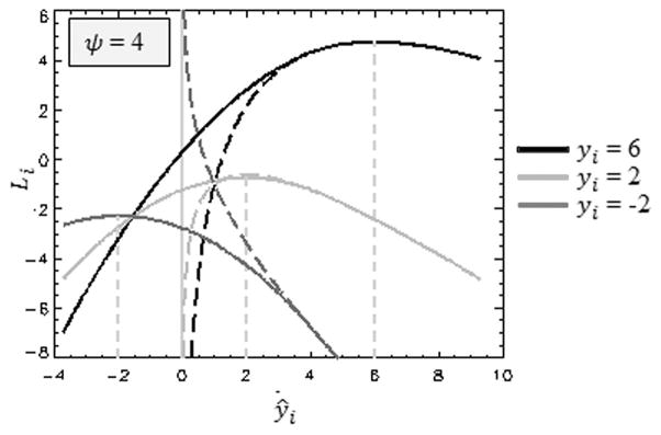
Standard likelihood function (dashed lines) is drawn for yi = 6 (black), yi = 2 (light grey), and yi = −2 (dark grey). Corresponding modified likelihood functions with ψ = 4, as proposed in (6), are drawn as solid lines.
Computing the reconstruction λ by maximizing the log-likelihood of (6) is not straightforward. Therefore, in every iteration n + 1, the objective function Lψ(ŷ;y) is approximated by the quadratic function Tψ(ŷ;ŷ(n), y) as follows:
| (7) |
where Di is independent of ŷi, and ŷ(n) denotes the calculated sinogram, obtained by applying (2) to the image λ(n) produced in iteration n. This function Tψ is equal to the likelihood Lψ in the current reconstruction and so are their first derivatives. Moreover, the derivatives of Lψ and Tψ have the same sign everywhere. Because they are both concave functions, this implies they have the same unique maximum
| (8) |
| (9) |
| (10) |
Using (2), Tψ(ŷ;ŷ(n), y) can be rewritten as a function of the new reconstruction λ. However, it is convenient to rewrite this new reconstruction as an update of the result from the previous iteration as follows:
| (11) |
where we introduced a set of αj ≥ 0 as design parameters. Now Tψ can be rewritten as a function of Δxj
| (12) |
To optimize T1, a gradient ascent algorithm as described in [13], [15], is applied. First, a series expansion of T1 around Δx = 0 is computed, applying the chain rule and noting that ∂ŷi/∂Δxj = αjcij is a constant [see (2)]
where the derivatives are evaluated in ŷ = ŷ(n). Since T1 is a quadratic function, the second-order expansion is exact. The second derivative of Tψ is always negative
| (13) |
Using in addition the inequality 2ΔxjΔxk ≤ (Δxj)2 + (Δxk)2, a surrogate function T2 for T1 can be defined. This surrogate function is equal to T1 in the current reconstruction λ(n) and lies below T1 elsewhere
| (14) |
| (15) |
Maximization of T2 is guaranteed to increase T1. Because every term of T2 depends on a single Δxj only, maximization of T2 is straightforward and yields
| (16) |
Using (11) and expanding the derivatives produces the new version of the NEGML algorithm
| (17) |
The original NEGML algorithm [13] is obtained when setting ψ = 1 and αj = 1. Neither ψ nor αj were explicit parameters in the original NEGML work. Instead of using ψ, division by zero was avoided by restricting the denominator to values larger than or equal to 1. Since ŷi is a number of photons, ŷi ≥ 1 was chosen as a reasonable value and gave good results. In other implementations of NEGML, this restriction was sometimes set at much smaller values e.g., ŷi ≥ 10−4 [11]. The results of different implementations were different regarding bias reduction, probably due to the different restriction for the denominator. The experiments in this work will explicitly test the influence of ψ on convergence and bias values.
When only using the Poisson likelihood, i.e., ŷi ≥ ψ for all i, and by using and ri = 0, the update becomes the MLEM update. The original NEGML algorithm used a mixed update step to improve the convergence in high activity regions. The update obtained for MLEM and NEGML were both calculated for voxel j and the largest of both was applied. This mixed update is equivalent to over-relaxation and might cause convergence problems. Hence, we prefer to use a pure NEGML update.
The convergence of high activity regions could be improved by altering the values for αj. This parameter was introduced in our work on metal artifact reduction and iterative reconstruction in CT [15], [16] and serves as a voxel convergence weight during reconstruction. Similar weights were used in the grouped coordinate algorithm by Fessler et al. [17]. Choosing gives the weighting used in MLEM, choosing αj = 1 results in the weighting of the original NEGML algorithm. A compromise could be obtained by defining weights that have a weaker dependence on the activity but still assign higher weights to high activity regions.
NEGML can be accelerated with ordered subsets, similarly as proposed for MLEM by Hudson and Larkin in [18].
B. AML
The ABML algorithm presented by Byrne [9] allows to perform an MLEM-like reconstruction between an image upper bound B and lower bound A by optimizing a well-chosen combination of KL distances (see [9]). This KL cost function can be considered as the sum of KL distances between yi and ŷi, using A and B as offsets. ABML can be seen as an extension of the MLEM algorithm, because when using the natural boundaries for MLEM, A = 0 and B = ∞, the KL cost function is equal to the Poisson likelihood and ABML becomes equivalent to MLEM.
The ABML reconstruction formula as used by Erlandsson et al. in [10] is
| (18) |
with
| (19) |
ABML can be used as a bias reduction algorithm by setting Aj to negative values. This way it allows for negative values in the image and the sinogram domain. It has been shown to reduce bias substantially [10], [11]. Often a single value for Aj is chosen, i.e., Aj = A for all voxels. This sets the lower limit for the reconstruction values to A and for the sinogram values to AΣkcik. Since there is no reason to have an upper bound for the image, Bj is usually set to a value much larger than the expected maximum activity. Introducing some approximations ABML can be extended to an ordered subsets version [10] with inclusion of randoms [11].
Since very large values are usually chosen for B, we propose to use ABML with infinite upper bound (as in MLEM), referred to as AML. This simplifies the expressions and avoids numerical problems that might occur for extreme values of B in (19). The AML update step for λj, with uniform A, in additive form becomes
| (20) |
This update step can be considered as an update where the image and sinogram are shifted, with A and AΣkcik respectively, for calculating the update step. This means that the Poisson distribution is evaluated at higher values where the influence of the non-negativity constraint is negligible. Before adding this to the current reconstruction the update is shifted back. Note that choosing A = 0 results in the original MLEM algorithm. The factor (λj − A)in (20) still represents an activity dependent weight for the update of voxel j, however, the weights become more uniform when A becomes more negative. Hong et al. [19] developed a variant of ABML that also allows for negative image values and reduces the influence of the non-negativity constraint during reconstruction by combining multiple time frames.
The parameter A is defined in image space. It is not straightforward to determine a lower bound such that bias-free images are ensured (i.e., such that negative values are not suppressed). To our knowledge no guidelines for choosing such a value for A have been published. When the lower bound is not low enough, bias might still occur. Therefore, A is usually set to a relatively extreme (negative) value to make sure that any constraint on the negativity has been eliminated. As argued in the next section, this turns the algorithm effectively into a least squares algorithm. It is unclear if such an extreme value is the best choice.
C. Unweighted Least Squares and Extreme Values for ψ and A
The influence of the parameter ψ and A on the reconstructions of NEGML and AML will be studied in this paper. The behavior of NEGML and AML for extremely high values for ψ and extremely low values of A will be studied as well. For large ψ, all sinogram pixels will be in the Gaussian regime. It is therefore expected that NEGML will become more and more similar to unweighted least squares reconstruction. The same holds for AML. When |A| is large1, the shift from A will be so large that the difference in Poisson weighting will be very small, eliminating all weighting difference in practice.
The NEGML algorithm for αj = 1 with ψ → ∞ becomes
| (21) |
This update formula is used whenever ŷi ≤ ψ for all ŷi.
The AML algorithm with A → −∞ yields
| (22) |
Unlike for NEGML this formula is theoretically only valid when A = −∞ since all finite values for A will still follow the Poisson distribution at ŷi − AΣhcih. However, this distribution becomes very flat for large |A|. For comparison, the typical least squares algorithm has the following form:
| (23) |
with ρ a relaxation factor. The results in (21) and (22) resemble the least squares update, but are not identical to it. Only when Σkcik is constant, both algorithms yield the least squares expression.
D. Additive Contamination
The additive contamination ri can be modeled as in (2). This is often referred to as ordinary Poisson, because it assumes that the randoms term ri is not noisy such that the Poisson model for yi is preserved. Ordinary Poisson is valid when an estimate of the randoms with low noise is available. This can be obtained by smoothing the randoms estimate [20] or by calculating them from the singles [21].
In some clinical PET systems, randoms precorrection is still applied. In this case, the randoms estimate is subtracted from the measurement, possibly leading to negative values in yi. For reconstruction with MLEM, these values should be set to zero which already introduces bias in the data. FBP, NEGML, and AML support negative sinogram values and no positivity requirement is needed. In [22] some modified statistical methods are given that specifically model randoms-precorrected PET emission data.
In the experiments described below, three different ways to correct for the randoms have been considered for the different reconstruction algorithms. For FBP, the randoms were always subtracted, with or without randoms smoothing. Since a uniform randoms contribution was used, this smoothing can be done with a Gaussian function. More dedicated smoothing algorithms have been developed for real PET systems [20]. For the iterative algorithms the following reconstructions can be used, where si is the noisy estimate of the randoms and is a smoothed randoms estimate (full-width half-maximum (FWHM) = 5 pixels).
Randoms precorrection with randoms smoothing: .
Ordinary Poisson with randoms smoothing: yi and .
Ordinary Poisson without randoms smoothing: yi and ri = si.
III. Experiments
This section describes the experiments that are performed to evaluate the bias reduction capacity of NEGML and AML, compared to FBP and MLEM. The experiments are based on 2-D simulations and consider the influence of the parameter ψ and A on the bias, variance, convergence and noise characteristics of NEGML and AML, respectively, for two different phantoms simulated with different settings.
A. Phantom 1
1) Simulations
A 2-D phantom with a cold, warm, and hot region, as shown in Fig. 2, is simulated. The activity in the image in activity per voxel is: 0 for the cold region, 1 for the warm region, and 4 for the hot region. The phantom is discretized in an image of 46 cm × 46 cm. During simulation this image was represented by a 920 × 920 pixel grid and a parallel beam simulation is performed with 920 lines of response per projection and 200 projections. Uniform water attenuation is applied. A uniform randoms contribution was simulated, assuming a Poisson distribution with the expectation equal to the mean of the uncontaminated sinogram. The system resolution was modeled by a Gaussian with FWHM of 5 mm.
Fig. 2.
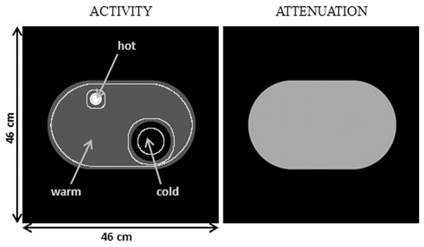
Phantom 1. Phantom has a cold, warm, and hot region. Activity for the main experiment was 0 for the cold region, 1 for the warm region, and 4 for the hot region. In a second setting, the phantom’s activity was multiplied by three. Phantom is assumed to have uniform water attenuation.
The obtained sinogram is rebinned to 230 lines of response per projection and 200 projections. This means that the simulation was four times oversampled. This simulation was repeated for 60 (Poisson) noise realizations and 50 time frames of increasing duration, resulting in data sets with mean count per sinogram pixel between 0.05 and 1000 counts. In a second simulation setting for this phantom, the activity in the image was multiplied by three.
2) Reconstructions
Reconstructions were performed with FBP, MLEM, NEGML, and AML on a 230 × 230 pixel grid, with pixel size 2 mm × 2 mm. FBP was performed using a standard ramp filter. For NEGML different values of ψ were evaluated: ψ = {1, 4, 9, 16, 25, 100, 100000}, αj = 1 was used for all j. For AML different values of A where used: A = {−1, −5, −10, −50, −100, −1000, −100000}. For all iterative methods 200 iterations were applied without the use of ordered subsets. During reconstruction the resolution was modeled by a Gaussian with FWHM 4 mm, introducing a small mismatch with the resolution of the simulation.
The simulations were reconstructed with three different ways of randoms handling, as listed in Section II-D.
3) Evaluation
A cold, warm and hot region of interest (ROI) are defined in the phantom. The ROIs exclude all pixels close to the edges, as shown in Fig. 2. The bias is estimated by calculating the mean value in a ROI over the different noise realizations, the ROI mean, defined by
| (24) |
with N the number of noise realizations and JROI the total number of pixels in the region. The ROI mean values are calculated for all 50 frames. The variance of the mean value over the noise realizations, the ROI Var, is calculated by
| (25) |
B. Phantom 2
This experiment is designed to further investigate whether the findings for phantom 1 and for the configuration described in the previous section, remain valid for other configurations. We will investigate whether changes in the number of projection lines (i.e., projection angles) for a fixed number of total counts has influence on the results. This will give an indication whether the results obtained in this study can be extended to fully 3-D PET and time-of-flight PET, where the ratio of the number of sinogram pixels to the number of image voxels is much larger than in 2-D PET. Because 3-D (TOF) PET simulations are very time consuming, it is more practical to study this effect by simulating 2-D PET with a much larger number of angles.
A different phantom with one cold and one warm region and three different projection settings are used for this experiment.
1) Simulations
A simple 2-D phantom consisting of a uniform disk with one cold region, depicted in Fig. 3, is simulated. The activity in the warm region is set to 1, in the cold region it is set to 0. The phantom is discretized in an image of 20 × cm 20 cm using a 400 × 400 pixel grid.
Fig. 3.
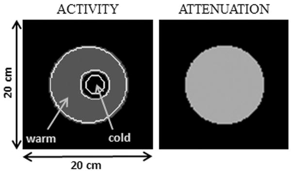
Phantom 2. Phantom consists of a warm and cold region. Activity and attenuation are shown. Phantom is assumed to have uniform water attenuation.
To evaluate the dependence on the sinogram pixel values this phantom was simulated with three different settings. For setting 1, 100 projection angles were calculated, 500 for setting 2, and 1000 for setting 3. However, the total number of counts for each simulation was kept constant, i.e., the sensitivity of each line of response of the simulated PET system was five times lower for setting 2 and 10 times lower for setting 3.
A parallel beam simulation with 400 lines of response per projection, was performed, assuming that the phantom was a uniform attenuator (consisting of water). A uniform randoms estimate was set equal to the mean of the uncontaminated sinogram. This simulated estimate was subjected to Poisson noise. The simulation was rebinned for reconstruction to 100 projection lines per angle.
For all three settings, 100 noise realizations were performed for 20 time frames of increasing duration. Only relatively short time frames were considered with mean sinogram count between 0.05 and 10 counts per pixel.
The system resolution was again modeled by a Gaussian with FWHM of 5 mm.
2) Reconstruction
The simulated measurements were reconstructed on a 100 × 100 pixel grid (2 mm isotropic pixel size) with FBP, MLEM, NEGML (ψ = {1, 4, 16}, again with αj = 1 for all j) and AML (A = {−1, −5, −50}). Precorrection of the randoms, using smoothed randoms (FWHM = 5 pixels), was used for FBP, Ordinary Poisson with smoothed randoms (FWHM = 5 pixels) was applied for the iterative methods. Iterative reconstruction was performed for 20 iterations with 10 subsets. As for phantom 1, a small mismatch with the resolution in the simulation was created by using by a Gaussian with FWHM = 4 mm during reconstruction.
3) Evaluation
A warm and a cold ROI are defined as shown in Fig. 3. The ROI mean is calculated, as in (24). Note that although all three settings have the same total amount of activity in the image and the sinogram, the mean count per sinogram pixel is larger for settings with fewer projection views.
IV. Results
A. Phantom 1
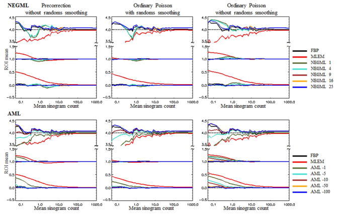
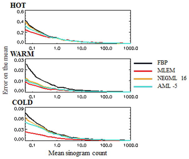
This section describes the main results of this work for the phantom depicted in Fig. 2. The ROI means as functions of the frame durations are shown in Fig. 4. The frame duration is represented by the mean number of sinogram counts in the frame. The standard error on the mean is given in Fig. 5
Fig. 4.
Phantom 1. Evaluation of the ROI Mean for different frame durations. Frame duration is represented by the mean number of counts per sinogram pixel in the frame. Three different ways for randoms handling are shown. Upper row gives the results for NEGML, the lower row shows the results for AML.
Fig. 5.
Phantom 1. Standard error on the mean for the Ordinary Poisson method with randoms smoothing (Fig. 4) for FBP, MLEM, NEGML 16, and AML −5 in the cold, warm, and hot region of phantom 1.
| (26) |
The results for ordinary Poisson with and without smoothed randoms and for randoms precorrection are shown. The upper row of the figure evaluates different values for ψ in NEGML, in comparison with FBP and MLEM. The lower row gives the evaluation of AML for different values of A.
Ordinary Poisson with randoms smoothing has the lowest bias for all methods. In general MLEM has the highest bias, especially in the cold and warm region. The bias of NEGML and AML is dependent on the model parameter. The positive bias in the cold region is higher when the data are noisier. Evaluating the bias in the cold region with respect to the expected value in the warm region, 40%–60% bias is observed for low count data. The bias only drops below 10% at on average 10 counts per sinogram pixels. The bias in the warm region is less pronounced, lower than 10%, for ordinary Poisson with randoms smoothing. It increases up to 40% for Ordinary Poisson without randoms smoothing and precorrection for very low count data. For NEGML all methods perform similarly with bias in the cold region mostly less than 2% (compared to the warm region). When the mean sinogram count has a value around ψ, a local increase in the bias can be observed. This is the most obvious in case of unsmoothed randoms. This local increase becomes less pronounced as ψ increases. We have currently no good explanation for this behavior. AML is dependent on A for bias reduction, the bias decreases with increasing |A|. This effect is again the most pronounced in case of unsmoothed randoms. For high values of |A| the bias is also below 2% everywhere and increases when |A| decreases.
In the hot region, even at relatively high counts, some remaining bias, of about 2%, is observed for NEGML and for AML with large |A|. This bias reduces when the number of iterations increases (data not shown). For less noisy data, MLEM performs in general better than both NEGML and AML in the high activity region. Note that there seems to be positive bias in the high activity region for FBP. However, this is a random error, caused by the high amounts of noise and the limited number of noise realizations. We verified this with additional noise realizations for low counts (data not shown).
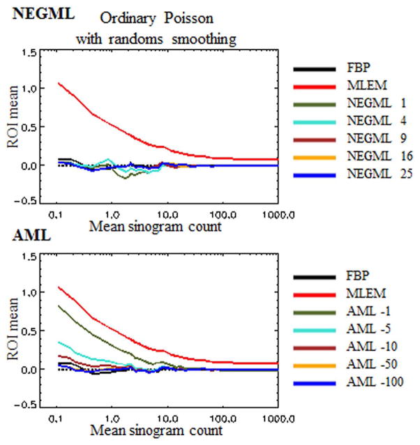
Fig. 6 depicts the ROI Mean as a function of the frame duration for the cold region of the same phantom with threefold increased activity reconstructed with Ordinary Poisson with randoms smoothing. In comparison with the phantom with lower activity, AML has more bias, which increases for smaller |A|. The results for NEGML are very similar to the case with less activity in the image. The reconstructions remain almost bias free. The difference between AML and NEGML for increased activity is due to the fact that was not changed while the activity in the image did change. The influence of increased activity on the bias in the warm and hot regions was less pronounced (not shown).
Fig. 6.
Phantom 1 with threefold increased activity. Evaluation of the ROI Mean for the cold regions for different frame durations with ordinary Poisson. Frame duration is represented by the mean number of counts per sinogram pixel in the frame. Upper row gives the results for NEGML, the lower row shows the results for AML.
The reconstructed images for the different methods with ordinary Poisson with randoms smoothing for on average five counts per sinogram pixel are shown in Fig. 7. After reconstruction, the images were smoothed with a Gaussian filter with FWHM of 4 mm. The maximum number of counts in this sinogram is 19 with more than 95% of the sinogram pixels below 16 counts. The typical noise-induced streaks are the most pronounced in the FBP reconstruction. MLEM suffers the least from these streaks. NEGML and AML have only few streaks for small ψ and small |A|. The streaks become more pronounced with increasing ψ or increasing |A|. AML has pixel dependent convergence weighting which means that it has more MLEM-like characteristics. The hot region is therefore sharper in MLEM and AML with small |A|. With respect to noise streaks there is no obvious difference observed between bias-free NEGML and AML images, only that AML has somewhat more streaks in the background of the image.
Fig. 7.
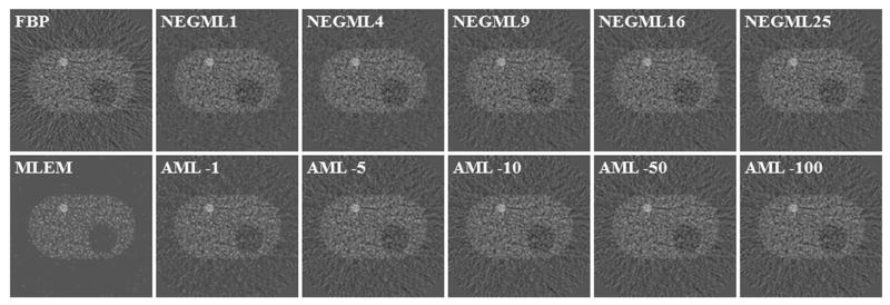
Phantom 1. FBP, MLEM, NEGML (ψ = {1, 4, 9, 16, 25}), and AML reconstruction (A = {−1, −5, −10, −50, −100}). Ordinary Poisson with randoms smoothing.
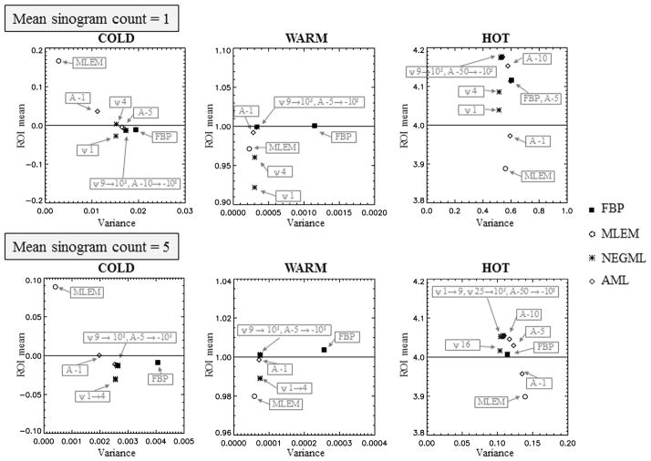
The influence of the parameter ψ or A on the ROI Mean and ROI Var is shown in Fig. 8. The frames represented in this figure have on average 1 or 5 counts per sinogram pixel. The variance in the cold and warm region is lower for NEGML and AML compared to FBP but still higher than for MLEM. For most parameter choices, the bias in NEGML and AML is better than for MLEM in the cold and warm regions. A local increase of the bias was observed when the mean sinogram count is close to the chosen value of ψ, the higher the value of ψ the smaller this increase in bias. This local increase is negligible from ψ = 16 and larger. The bias due to incomplete convergence in the hot region, for NEGML and AML with large |A|, was expected from previous results.
Fig. 8.
Phantom 1. Mean with respect to variance in the cold regions, warm region and hot region for different values of ψ and A. Chosen frame duration correspond to on average 1 and 5 counts per sinogram pixel. Solid line represent the true value for each region. Ordinary Poisson with randoms smoothing.
The influence of ψ and A on the convergence of NEGML and AML for all three regions is given in Fig. 9, for a measurement with on average five counts per sinogram pixel. The result is shown for ordinary Poisson with randoms smoothing and for parameters: ψ = {4, 25} and A = {−1, −10, −105}. For this frame duration NEGML with ψ = 25 worked completely in the Gaussian regime. The convergence for the cold and warm region is relatively fast. At 50 iterations all methods converged. In the hot regions MLEM and AML with small |A| converge faster than NEGML and AML with larger |A|. An experiment with more iterations (not shown) indicates that most of the algorithms were not yet converged in the hot region, another 100–200 iterations are needed to obtain complete convergence and a hot region without bias.
Fig. 9.
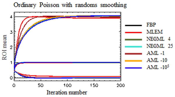
Phantom 1. Convergence of MLEM, NEGML (with ψ = {4, 25}), and AML (with A = {−1, −10, −105}). Value for FBP is given as a reference.
B. Phantom 2
The graphs in Fig. 10 depict the ROI mean in the cold and warm region of phantom 2 for a set of short frame durations for FBP, MLEM, NEGML, and AML. Three different projection setting, with a different number of projection angles were used.
Fig. 10.
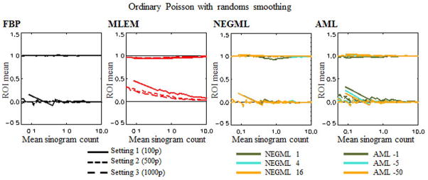
Phantom 2. ROI mean in the cold and warm region for three setting. Setting 1: 100 projections angles (solid line), setting 2: 500 projection angles (small dashes), setting 3: 1000 projection angles (long dashes).
FBP and NEGML show similar bias reduction for all three settings. For the smaller parameters, ψ = {1, 4}, again a local increase is observed, this is the most obvious for the warm region. For ψ = 16 no bias is observed for all three settings. The bias for MLEM and AML is not the same for all three settings. Although the activity in the image is the same for all settings, the same value for A results in different bias reduction depending on the setting. The largest value of |A|, A = −50, results in bias-free reconstruction for all three settings.
V. Discussion
Two methods for bias reduction have been presented. They both use a likelihood function which can be considered as a modified Poisson function.
NEGML uses a combination of a Poisson and Gaussian function with a transition between both functions at ψ such that negative sinogram values are allowed. AML is a modification of ABML with upper bound B set to infinity, which simplifies and stabilizes (numerically) the algorithm. AML can be considered to apply a shift on the data such that they are evaluated at higher values where the influence of the positivity constraint is negligible.
The influence of the parameters ψ and A on the bias in the reconstructed images has been investigated. It was shown that both algorithms converge to least squares-like algorithms when their parameter is sufficiently large.
For NEGML, very low bias was observed for most values of ψ. For low values of ψ, a (so far unexplained) increase in bias was seen when the mean sinogram count was similar to ψ. Consequently, sufficiently large negative values should be allowed to ensure bias-free reconstructions; ψ =16 was found to result in bias-free images under all circumstances. Note that the original NEGML method [13] implicitly used ψ =1 and that it was sometimes also used with even smaller values of ψ (e.g., 10−4 in [11]) leading to remaining bias in the images.
Small values for |A| in AML result in MLEM-like reconstruction properties, gradually increasing |A| yields a transition to least squares reconstruction properties. When |A| is sufficiently large, bias-free reconstructions are obtained. Note that in this work a fixed value for A was chosen. Studying the influence of an nonuniform image Aj with j = 1 … J, was beyond the scope of this paper.
For both algorithms large values for their parameter yield bias-free images. It turned out that least-squares-like behavior is required to obtain bias-free images. Both for NEGML and AML this bias-reduction comes at the cost of increased variance. No situation could be found where NEGML and AML have equal bias properties but significantly different variance behavior. Nevertheless, they both have lower variance than FBP, which is a useful property.
Parameters that give rise to bias-free NEGML and AML images often reduce the convergence rate of the hot region, even for relatively high counts. To reduce the required number of iterations ordered subsets can be used (to avoid limit cycle solutions the number of subsets could be decreased at higher iteration numbers). For NEGML, αj could be chosen non-uniformly but care has to be taken since convergence will be slowed down for voxels with relatively low αj. We tested some choices where αj increased monotonically with λj (data not shown), the results were comparable to the results for small |A| in AML: improved convergence in hot regions at the cost of risking more bias for cold regions.
This study also investigated the influence of the randoms handling on the bias in the image. The way the randoms are handled may have a large influence on the severeness of the bias. Ordinary Poisson with randoms smoothing copes best with noisy low count data. Ordinary Poisson without randoms smoothing shows the worst performance.
For precorrected data, the Shifted Poisson method as proposed by Yavuz and Fessler in [23] should be used instead of the Ordinary Poisson method. In a test using Shifted Poisson (data not shown), similar results have been obtained: the bias for Shifted Poisson without randoms smoothing was substantially increased compared to Shifted Poisson with randoms smoothing. The difference between Shifted Poisson and Ordinary Poisson was negligible compared to the difference between the use of unsmoothed and smoothed randoms. Randoms precorrection creates negative sinogram values, which must be set to zero in MLEM and therefore contribute a positive bias [5]. Since AML and NEGML can handle negative sinogram values, these algorithms do not encounter this problem. Under all circumstances both NEGML and AML (with large parameter) were able to mitigate the bias.
The experiments with the adjusted phantom 1 (threefold activity) and phantom 2 confirm the conclusions drawn for phantom 1, despite the fact that different activity and different projection settings were used. The experiments in this work have thus only been performed on 2-D data. However, a tenfold increase in the number of sinogram pixels for the same number of image pixels did not change the major results. Therefore, we anticipate that similar results will be obtained in 3-D and time-of-flight PET, where the ratio of sinogram pixels to image pixels is also much larger.
VI. Conclusion
Two algorithms are introduced that modify the Poisson likelihood in order to mitigate bias. Using very different mechanisms, both algorithms provide a kind of balance between the Poisson likelihood and the Gaussian likelihood (i.e., least squares), which is controlled by a single parameter.
NEGML combines a Poisson and Gaussian distribution and was shown to reduce the bias significantly when the parameter that determines the switch between both distributions, ψ, was at least equal to 16. AML is proposed as a simplification of ABML with upper bound B set to infinity. It results in bias-free images when the lower bound A is set low enough. Both algorithms are effective in reducing bias when their parameter was chosen high enough in magnitude. This comes at the cost of increased variance compared to MLEM but they both have lower variance than FBP.
Another issue that was studied was the influence of randoms handling. The use of unsmoothed randoms or randoms precorrected data increases the bias substantially. However, NEGML with ψ ≥ 16 and AML with a “sufficiently high” magnitude of A performed well for all randoms processing approaches.
Although the experiments in this work have been applied on 2-D data, the results suggested that the conclusion drawn may hold for 3-D and time-of-flight-PET configurations as well.
Footnotes
To avoid confusion when discussing negative values of A, |A| is used. Since this paper only considers negative values of A, |A| is unambiguous. Large |A| thus means a negative value of A with large magnitude.
Color versions of one or more of the figures in this paper are available online at http://ieeexplore.ieee.org.
Contributor Information
Katrien Van Slambrouck, Department of Imaging and Pathology, Division of Nuclear Medicine and Medical Imaging Research Center, K.U. Leuven, B-3000 Leuven, Belgium.
Simon Stute, CEA, DSV, I2BM, SHFJ, Orsay, F-91401, France.
Claude Comtat, CEA, DSV, I2BM, SHFJ, Orsay, F-91401, France.
Merence Sibomana, Sibomana Consulting SPRL, Emines, Belgium.
Floris H. P. van Velden, Department of Radiology and Nuclear Medicine, VU University Medical Center, 1007MB Amsterdam, The Netherlands
Ronald Boellaard, Department of Radiology and Nuclear Medicine, VU University Medical Center, 1007MB Amsterdam, The Netherlands.
Johan Nuyts, Email: johan.nuyts@uzleuven.be, Department of Imaging and Pathology, Division of Nuclear Medicine and Medical Imaging Research Center, K.U. Leuven, B-3000 Leuven, Belgium.
References
- 1.Qi J, Leahy R. Iterative reconstruction techniques in emission computed tomography. Phys Med Biol. 2006;51(15):R541–578. doi: 10.1088/0031-9155/51/15/R01. [DOI] [PubMed] [Google Scholar]
- 2.Shepp LA, Vardi V. Maximum likelihood reconstruction for emission tomography. IEEE Trans Med Imag. 1982 Oct;1(2):113–122. doi: 10.1109/TMI.1982.4307558. [DOI] [PubMed] [Google Scholar]
- 3.Lange K, Carson R. EM reconstruction for emission and transmission tomography. J Comput Assist Tomogr. 1984;8(2):306–316. [PubMed] [Google Scholar]
- 4.Boellaard R, van Lingen A, Lammertsma AA. Experimental and clinical evaluation of iterative reconstruction (OSEM) in dynamic PET: Quantitative characteristics and effects on kinetic modeling. J Nucl Med. 2001;42(5):808–817. [PubMed] [Google Scholar]
- 5.van Velden FHP, Kloet RW, van Berckel BNM, Wolfensberger SPA, Lammertsma AA, Boellaard R. Comparison of 3D-OP-OSEM and 3D-FBP reconstruction algorithms for high-resolution research tomograph studies: Effects of randoms estimation methods. Phys Med Biol. 2008;53:3217–3230. doi: 10.1088/0031-9155/53/12/010. [DOI] [PubMed] [Google Scholar]
- 6.Reilhac A, Tomeï S, Buvat I, Michel C, Keheren F, Costes N. Simulation-based evaluation of OSEM iterative methods in dynamic brain PET studies. NeuroImage. 2008;39:359–268. doi: 10.1016/j.neuroimage.2007.07.038. [DOI] [PubMed] [Google Scholar]
- 7.Barrett H, Myers K. Foundations of Image Science. Hoboken, NJ: Wiley; 2004. [Google Scholar]
- 8.Cloquet C, Defrise M. MLEM and OSEM deviate from the Cramer-Rao bound at low counts. IEEE Trans Nucl Sci. 2013 Feb;601:134–143. [Google Scholar]
- 9.Byrne C. Iterative algorithms for deblurring and deconvolution with constraints. Inverse Problems. 1998;14:1455–1467. [Google Scholar]
- 10.Erlandsson K, Visvikis D, Waddington W, Cullum I, Jarritt P, Polowsky L. Low-statistics reconstruction with AB-EMML. IEEE Nucl Sci Symp Conf Rec. 2000;2:15/249–253. [Google Scholar]
- 11.Verhaeghe J, Reader A. AB-OSEM reconstruction for improved Patlak kinetic parameter estimation: A simulation study. Phys Med Biol. 2010;55:6739–6757. doi: 10.1088/0031-9155/55/22/009. [DOI] [PubMed] [Google Scholar]
- 12.Rahmim A, Zhou Y, Tang J, Lu L, Sossi V, Wong DF. Direct 4D parametric imaging for linearized models of reversibly binding PET tracers using generalized AB-EM reconstruction. Phys Med Biol. 2012;57:733–755. doi: 10.1088/0031-9155/57/3/733. [DOI] [PMC free article] [PubMed] [Google Scholar]
- 13.Nuyts J, Stroobants S, Dupont P, Vleugels S, Flamen P, Mortelmans L. Reducing loss of image quality due to the attenuation artifact in uncorrected PET whole body images. J Nucl Med. 2002;43:1054–1062. [PubMed] [Google Scholar]
- 14.Grèzes-Besset L, Nuyts J, Boellaard R, Buvat I, Michel C, Pierre C, Costes N, Reilhac A. Simulation-based evaluation of NEG-ML iterative reconstruction of low count PET data. Nucl Sci Symp Conf Rec. 2007:3009–3014. [Google Scholar]
- 15.Van Slambrouck K, Nuyts J. Reconstruction scheme for accelerated maximum likelihood reconstruction: The patchwork structure. IEEE Trans Nucl Sci. 2014 Feb;61(1):173–181. [Google Scholar]
- 16.Van Slambrouck K, Nuyts J. Metal artifact reduction in computed tomography using local models in an image block-iterative scheme. Med Phys. 2012;39(11):7080–7093. doi: 10.1118/1.4762567. [DOI] [PubMed] [Google Scholar]
- 17.Fessler JA, Ficaro EP, Clinthorne NH, Lange K. Grouped-coordinate ascent algorithm for penalized-likelihood transmission image reconstruction. IEEE Trans Med Imag. 1997 Apr;16(2):166–175. doi: 10.1109/42.563662. [DOI] [PubMed] [Google Scholar]
- 18.Hudson H, Larkin R. Accelerated image reconstruction using ordered subsets of projection data. J Theoret Biol. 1994;13(4):601–609. doi: 10.1109/42.363108. [DOI] [PubMed] [Google Scholar]
- 19.Hong I, Cho S, Casey M, Michel C. Complementary reconstruction: Improving image quality in dynamic PET studies. IEEE Nucl. Sci. Symp. Med. Imag. Conf; Valencia, Spain. 2011; pp. 4327–4328. [Google Scholar]
- 20.Watson C. Co-fan-sum ratio algorithm for randoms smoothing and detector normalization in PET. IEEE Nucl. Sci. Symp. Conf. Rec; Knoxville, TN. 2010; pp. 3326–3329. [Google Scholar]
- 21.Stearns C, McDaniel D, Kohlmeyer S, Arul P, Geiser B, Shanmugan V. Random coincidence estimation from single event rates on the discovery ST PET/CT scanner. IEEE Nuclear Sci. Symp. Conf. Rec; Portland, OR. 2003; pp. 3067–3069. [Google Scholar]
- 22.Ahn S, Fessler J. Emission image reconstruction for randoms-precorrected PET allowing negative sinogram values. IEEE Trans Med Imag. 2004 May;23(5):591–601. doi: 10.1109/tmi.2004.826046. [DOI] [PubMed] [Google Scholar]
- 23.Yavuz M, Fessler J. Statistical image reconstruction methods for randoms-precorrected PET scans. Med Image Anal. 1999;2(4):369–378. doi: 10.1016/s1361-8415(98)80017-0. [DOI] [PubMed] [Google Scholar]


