Cortical Folding Development Study based on Over-Complete Spherical Wavelets

Abstract

We introduce the use of over-complete spherical wavelets for shape analysis of 2D closed surfaces. Bi-orthogonal spherical wavelets have been shown to be powerful tools in the segmentation and shape analysis of 2D closed surfaces, but unfortunately they suffer from aliasing problems and are therefore not invariant under rotations of the underlying surface parameterization. In this paper, we demonstrate the theoretical advantage of over-complete wavelets over bi-orthogonal wavelets and illustrate their utility on both synthetic and real data. In particular, we show that over-complete spherical wavelets allow us to build more stable cortical folding development models, and detect a wider array of regions of folding development in a newborn dataset.

1. Introduction

The Euclidean wavelet transform [1] is a powerful tool in image processing that decomposes a signal into component signals of different scales and spatial locations. It has been widely applied to compression, de-noising, and medical image analysis [2–4].

In the past decade, there has been much work on extending the general paradigm of linear filtering to the spherical domain. For example, the lifting scheme in [5] adopts a non-parametric approach to computing a wavelet decomposition of arbitrary meshes by generalizing the standard 2-scale relation of the Euclidean wavelets, enabling a multiscale representation of the original mesh (image) with excellent compression and speed performance. The resulting bi-orthogonal spherical wavelet transform has been successfully applied to the segmentation and shape analysis of 2D closed surfaces in medical imaging [6, 7]. In particular, the use of spherical wavelet transform in cortical shape analysis allows us to study cortical folds of different spatial scales, which are difficult to analyze by cortical folding analysis methods based on local features such as curvature and sulcal depth measurements.

Unfortunately, the bi-orthogonal spherical wavelet transform is not rotationally invariant under rotations of the surface parameterization. Since we are considering 2D closed surfaces with spherical topology, a natural parameterization is a 1-1 mapping to the sphere. The rotation of surface parameterization refers to the rotation of the underlying spherical coordinate system. Figure 1 shows a toy example that illustrates the sensitivity of bi-orthogonal wavelets to the rotation of surface parameterization. We first generate a bump centered at the north pole on a sphere, as shown in Figure 1(a). We then apply the bi-orthogonal wavelet transform to both the original surface and the reparameterized surface where the spherical coordinate is rotated by an arbitrary angle. Figure 1(b) and 1(c) show the low level (coarse scale) bi-orthogonal wavelet coefficients that have significant magnitude before and after the rotation of surface parameterization. With the original parameterization, we can accurately detect the location of the bump since only the wavelet coefficient at the center of the bump has large magnitude, illustrated by a single bright spot in Figure 1(b). However, with the rotation of parameterization, two wavelet coefficients have significant magnitude, as shown by the two bright spots in Figure 1(c).

Figure 1.

The comparison of bi-orthogonal and over-complete spherical wavelets in detecting local shape variation. (a) Synthetic surface with a bump. (b) The bi-orthogonal wavelet coefficient that has the largest magnitude when the north pole of surface mesh is right underneath the center of bump. (c) The bi-orthogonal wavelet coefficients with large magnitude when the surface parameterization is rotated. (d) The over-complete wavelet coefficients that have the largest magnitude with or without the rotation of surface parameterization.

The bi-orthogonal wavelet transform is not invariant under rotations of the underlying parameterization because it subsamples the signal progressively when decomposing it at the lower frequency (coarser) levels. This subsampling causes aliasing at all the single frequency levels although all the levels, when combined, add up to an invertible transform. This is problematic since being able to analyze the wavelet coefficients at each individual frequency level is one of the advantages of wavelet transform. Consequently, surface analysis results can vary significantly with the rotation of surface parameterization and one loses the ability to accurately localize geometric effects of interest.

The aliasing of individual levels of orthogonal and bi-orthogonal wavelets is a well-known problem in the Euclidean domain. Over-complete wavelets, such as the steerable pyramid proposed by Simoncelli et al. [8], are useful for solving the aliasing problem.

Recently, the corresponding steerable pyramid in the spherical domain was proposed by Antoine et al. [9] and discretized by Bogdanova et al. [10] for axis-symmetric wavelets. Unlike the steerable pyramid, their method of construction is grounded in group or representation theory. In this paper, we propose to use the over-complete wavelets introduced by Yeo et al. [11]. Their over-complete wavelets are based on filter bank theory, directly extending the ideas of Simoncelli to the sphere. In this work we only consider invertible axis-symmetric wavelets which are not necessarily self-invertible. We note that axis-symmetric spherical wavelets are symmetrical about the north pole.

With the over-complete wavelet transform, we can always accurately detect the single bump, as shown in Figure 1(d), regardless of the rotation of the underlying surface parameterization. The over-complete wavelet transform achieves such invariance by sufficiently sampling at each level of the wavelet transform.

In the following section, we introduce the construction of both wavelets, and theoretically prove the invariance property of the over-complete wavelet transform. In section 3, we describe the use of both wavelets in building cortical folding development models in a newborn dataset. Finally in section 4, we show the advantage of the over-complete wavelets in providing more accurate and sensitive results for the folding development study.

2. Methods

For closed 2D surface that has a spherical topology, various methods have been developed to impose a spherical coordinate system on the surface [12, 13]. In the underlying spherical coordinate system, we can use {X (θ_i, ϕ_i), Y (θ_i, ϕ_i),Z (θ_i, ϕ_i)} to denote the set of mesh vertices indexed by i. Many parametric mesh representations have been proposed, including spherical harmonics [12], polynomials [14] and bi-orthogonal spherical wavelets [6, 7], to transform or decompose the individual coordinate functions X (θ_i, ϕ_i), Y (θ_i, ϕ_i) and Z (θ_i, ϕ_i) separately.

We employ the over-complete wavelet transform to define local decomposition of the surface. We use the resulting wavelet coefficients of the coordinates for shape analysis. Without loss of generality, we introduce both the bi-orthogonal and over-complete spherical wavelet transforms for a generic scalar spherical function f (θ, ϕ) in the following two subsections.

2.1. Bi-orthogonal spherical wavelet transform

The bi-orthogonal spherical wavelets employed in this paper belong to the second generation wavelets, which no longer rely on the adaptive constructions based on traditional dilation and shifting, but still maintain the notion that a basis function at a certain level can be expressed as a linear combination of basis functions at a finer, more subdivided level.

The construction of these spherical wavelets relies on a recursive subdivision of an icosahedron (subdivision level 0). Denoting the set of all vertices on the mesh before the j^th subdivision as K(j), a set of new vertices M(j) can be obtained by adding vertices at the midpoint of edges and connecting them with geodesics. Therefore, the complete set of vertices at the (j+1)^th level is given by K (j + 1) = K (j) ∪ M (j). As a result, the number of vertices at level j is 10 × 4^j + 2, e.g., 12 vertices at level 0, 42 at level 1, 162 at level 2, etc.

Next, by using an interpolating subdivision scheme and the lifting scheme, we can construct a set of wavelet functions ψ_j,m at levels j = −1, …, J and node m ∈ M (j) on the subdivided icosahedron surfaces. At the coarsest level −1, the wavelet functions are actually the scaling functions at the level 0, and we denote M (−1) = K (0) to facilitate notation. Any function f with finite energy can then be decomposed as a linear combination of these basis functions:

$$f=\sum _{j=-1,\dots ,J,m\in M(j)}{\gamma }_{j,m}{\psi }_{j,m},$$ (1)

where γ_j,m is the wavelet coefficient at level j and node m ∈ M (j).

In practice, we first interpolate the input spherical function onto a subdivided icosahedron mesh, and then carry out the forward and inverse wavelet transforms using the interpolation subdivision and lifting scheme, without explicit construction of the wavelet functions [5].

2.2. Over-complete spherical wavelet transform

The construction of the over-complete spherical wavelet function is based on the general continuous filter bank theory [11]. Continuous spherical function f (θ, ϕ) is projected onto the space of N spherical analysis filters ${\{{\tilde{h}}_n(\theta ,\varphi )\}}_{n=1}^N$ by performing a spherical convolution between f (θ, ϕ) and each analysis filter h̃_n (θ, ϕ).

In the case of axis-symmetric spherical filters, the convolution outputs are also spherical images ${\{g_n(\theta ,\varphi )\}}_{n=1}^N$. We can then perform an inverse spherical convolution between each convolution output g_n (θ, ϕ) and corresponding spherical synthesis filter h_n (θ, ϕ), and obtain a reconstructed image f̑ (θ, ϕ) by summing the outputs of the inverse spherical convolution. The system of forward and inverse spherical convolutions, using analysis and synthesis filters respectively, is invertible if f̑ is equal to f.

We define the system of spherical filters to be an over-complete forward and inverse wavelet transform if it is invertible and the analysis filters ${\{{\tilde{h}}_n(\theta ,\varphi )\}}_{n=1}^N$ are dilated versions of a mother wavelet.

For this work in particular, we choose the Laplacian-of-Gaussian on the plane as our mother wavelet. We then perform the usual dilation on the plane to generate the differently dilated daughter wavelets. At last, we stereographically project the set of wavelets onto the sphere to obtain the corresponding wavelet analysis filters. This process of dilation via the plane is known as stereographic dilation and is utilized because dilation on a sphere is necessarily non-linear [9–11].

Noting that the spherical harmonics are a set of orthonormal basis for functions on L² (S²) and denoting by h^l,m the spherical harmonic coefficient of degree l and order m of a spherical function h, we define the synthesis filters to be [11]:

$$h_n^{l,m}=\{\begin{array}{cc}\hfill \frac{1}{H_{\tilde{h}}(l)}{\tilde{h}}_n^{l,m}\hfill & \mathit{\text{for}}{H}_{\tilde{h}}(l)>0,\hfill \\ \hfill 0\hfill & \mathit{\text{otherwise}}\hfill \end{array}$$ (2)

where

$$H_{\tilde{h}}(l)=\frac{8{\pi }^2}{2l+1}\sum _{n=1}^N\sum _{m\prime =-1}^l|{\tilde{h}}_n^{l,m\prime }{|}^2.$$ (3)

Therefore, by using equation (2) and (3) to construct the synthesis filters, we ensure that our over-complete wavelets are invertible, as proved by Yeo et al. in [11].

Since our wavelet analysis filters are axis-symmetric, the forward and inverse continuous wavelet transform can be performed in the spherical harmonic domain [11, 15]. Thus, the original function f, the reconstructed function f̑ and the wavelet coefficient g can be represented by their spherical harmonic coefficients of degree l and order m as f^l,m, f̂^l,m and g^l,m respectively.

Since the wavelet transform is conducted in the spherical harmonic domain, in practice, we first re-interpolate the surface mesh onto a latitude-longitude grid, and then use the publicly available program S2kit [16] to perform the fast discrete spherical harmonic transform [15]. Because the latitude-longitude grid is denser near the poles than at the equator, we ensure sufficient samples at the equator to avoid aliasing.

Since the purpose of wavelet decomposition is to analyze the underlying function locally in both space and frequency, we use S2kit to transform the acquired wavelet coefficients g_n^l,m, at each level n back to the latitude-longitude grid {g_n (θ_j, ϕ_j)}. We note that the inverse spherical harmonic transform is invertible via the sampling theorem of Driscoll and Healy [15] and thus we do not lose any information by working in the spatial domain. Therefore, we can equivalently think of {g_n (θ_j, ϕ_j)} as over-complete discrete wavelet transform.

In some cases, it might be more efficient to analyze the wavelet coefficients on a more uniform grid. In our work, we re-interpolate the wavelet coefficients samples on the latitude-longitude grid onto a subdivided icosahedron grid of high enough resolution. In our experiments, the re-interpolating process has little effects on the analysis as long as the samples are sufficiently dense relative to the size of the geometric features of interest.

2.3. Rotational invariance and aliasing

2.3.1. Rotating the surface

For the purpose of shape analysis, we apply the wavelet transformation to the individual coordinate functions X (θ_i, ϕ_i), Y (θ_i, ϕ_i) and Z (θ_i, ϕ_i) separately. Since both the bi-orthogonal and the over-complete spherical wavelet transforms are linear, we can show that

$$\mathrm{\Phi }(R([X({\theta }_i,{\varphi }_i);Y({\theta }_i,{\varphi }_i);Z({\theta }_i,{\varphi }_i)]))=R(\mathrm{\Phi }([X({\theta }_i,{\varphi }_i);Y({\theta }_i,{\varphi }_i);Z({\theta }_i,{\varphi }_i)]))$$ (4)

where Φ denotes the wavelet transform and R(·) denotes a rotation operator that rotates a point in 3D. Applying R(·) to {X, Y, Z} therefore rotates the surface in 3D.

Equation (4) implies that rotating a surface before the wavelet transformation is the same as applying a rotation after the wavelet transformation. Hence, both the bi-orthogonal and over-complete wavelet transforms are invariant under the rotation of 2D closed surfaces.

2.3.2. Rotating the surface parameterization

In contrast, the bi-orthogonal wavelet transform is not invariant under rotations of the surface parameterization, as demonstrated in the Introduction Section. This is because at each subsequent lower frequency level (coarser resolution), the input to the bi-orthogonal wavelet transform is implicitly a smooth sub-sampled version of the original function. However, despite the smoothing, the number of samples is insufficient to prevent aliasing. Therefore, when the surface parameterization is rotated, the sub-sampled spherical function and thus the wavelet coefficients can change substantially. As a result, the bi-orthogonal wavelet coefficients are not invariant under rotations of the surface parameterization, and the shape analysis results based on the bi-orthogonal wavelet transform depend on the arbitrary choice of the parameterization frame (origins and axes).

Because the bi-orthogonal spherical wavelet transform is computed implicitly rather than defined via sampling of the continuous convolution between a spherical function and the wavelet kernels, it is not trivial to artificially increase the number of samples at each level.

Conversely, the over-complete spherical wavelets are invariant under the surface parameterization since each level of the wavelet transform is sufficiently sampled.

Specifically, for the over-complete wavelet transform, we compute the wavelet coefficients g_n at level n by convolving the spherical function f with level n analysis filter h̃_n. Since the analysis filter is axis-symmetric, we can compute the convolution in the spherical harmonic domain as [17]:

$$g_n^{l,m}=\sqrt{\frac{4\pi }{2l+1}}{\tilde{h}}_n^{l,0*}{f}^{l,m}$$ (5)

Let Df be the rotation of the parameterization of a spherical image f by D. It can be shown that

$${(Df)}^{l,m}=\sum _{|m\prime |\le l}{D}_l^{mm\prime }{f}^{l,m\prime }$$ (6)

where $D_l^{mm\prime }$ denotes the Wigner-D function associated with the rotation D [17]. Combining equations (5) and (6), we obtain:

$$\sqrt{\frac{4\pi }{2l+1}}{\tilde{h}}_n^{l,0*}{(Df)}^{l,m}=\sqrt{\frac{4\pi }{2l+1}}{\tilde{h}}_n^{l,0*}\sum _{|m\prime |<l}{D}_l^{mm\prime }{f}^{l,m\prime }=\sum _{|m\prime |<l}{D}_l^{mm\prime }\sqrt{\frac{4\pi }{2l+1}}{\tilde{h}}_n^{l,0*}{f}^{l,m\prime }=\sum _{|m\prime |<l}{D}_l^{mm\prime }{g}^{l,m\prime }={(D{g}_n)}^{lm}.$$ (7)

Therefore, the over-complete wavelet transform is invariant under rotations of the underlying coordinate system. Although we sample the resulting wavelet transform as described in Section 2.2, the sampling theorem of Driscoll and Healy [15] ensures the process is lossless. Therefore the over-complete discrete wavelet transform is also rotationally invariant up to the spacing of the sampling grid. In practice, we over-sample to locate regions of interest to within the accuracy of the original surface parameterization, as described in Section 3.1.

To illustrate the advantage of over-complete wavelets over the bi-orthogonal wavelets in shape analysis, we compare the results of cortical folding development study using both wavelets in the following sections.

3. Experimental setup

3.1. Data and preprocessing

The dataset used in this study includes T1 weighted 3D MR images of eight normal neonates with corrected gestational ages (cGA) of 30.57, 31.1, 34, 37.71, 38.1, 38.4, 39.72, and 40.43 weeks, and 3 children who were 2, 3 and 7 years old (T2 weighted MR images not available for this dataset). We use Freesurfer [18] to preprocess this dataset, except that manual segmentation has to be done on the images of newborns due to inverted gray/white contrast. Based on the image segmentation, we reconstruct and refine the white/gray matter boundary, and use these white matter surfaces in our cortical shape analysis. We map the white matter surface onto a sphere and register all the surfaces in the spherical coordinate system [13, 19, 20]. We then apply a wavelet transform to the x, y and z coordinates of the surface points. Therefore, each output wavelet coefficient in this shape analysis is a vector with corresponding x, y and z components. In order to compare the bi-orthogonal and the over-complete wavelets in the cortical shape analysis, we generate a second set of white matter surfaces where the underlying spherical coordinate system is rotated by 30 degree around the x- and y- axes respectively.

For the bi-orthogonal wavelets used in this work, we employed the butterfly subdivision scheme and a lifting algorithm to ensure that the constructed wavelet function has one vanishing moment [5]. Before applying the forward wavelet transform, we first sample the registered white matter surface to an icosahedron at subdivision level 7 because it has a total number of 163,842 vertices and is thus sufficiently dense to represent the white matter surface reconstructed from ~1 mm isotropic MRI, which typically has about 120,000 vertices. Following the widely used convention, we index the resulting wavelet basis functions from level −1 to 6, and plot part of them in Figure 2(a).

Figure 2.

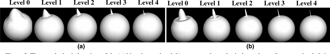
The wavelet basis functions of the (a) bi-orthogonal and (b) over-complete spherical wavelets at frequency levels 0–4.

For the over-complete wavelets, the smallest scale analysis filter is chosen to be the Laplacian of a Gaussian function with width 0.002 radian on the latitude-longitude grid. The wavelets at coarser levels are constructed by dilating the smallest scale wavelet subsequently by a factor of 2 each time. We index our over-complete wavelets from level −2 to 5 in order to match the spatial scales of the bi-orthogonal wavelets at the same levels, as shown in Figure 2(b). Before conducting the over-complete wavelet transform in the spherical harmonic domain using equation (5), we first sample the white matter surfaces onto a latitude-longitude grid of 10⁶ points and then transform them to the spherical harmonic domain using S2kit [16].

Finally, we apply these two wavelet transforms to the white matter surfaces with both the original and the rotated parameterizations to study the influence of this rotation on the results of folding development study.

3.2. Cortical folding development model

To quantitatively study the cortical folding development, which starts slowly, and accelerates before slowing down to approach a limit, we apply the widely accepted Gompertz model to the white matter surface in the wavelet domain [7]. Specifically, if w(t) is one of the spherical wavelet features extracted from a subject of age t, we use a Gompertz curve to model the evolution of this feature with age as follows:

$$w(t_i)=b_1{e}^{-e^{(-b_2(t_i-b_3))}}+\epsilon (t_i){,}_{i=1,\dots ,11}$$ (8)

where b₁ is the maximum value at maturation, b₂ is the growth rate that quantifies the speed of the folding development, b₃ is the inflexion point that indicates the age of the fastest folding development, and ε(t) represents additive zero-mean noise.

Due to the limited number of subjects available in this study, we apply a regularization framework for estimating parameter b₁, b₂ and b₃ to avoid overfitting. In such a framework, we minimize a cost function:

$$Q({\{b_j\}}_{j=1}^3)=\sum _{i=1}^N{(b_1{e}^{-e^{(-b_2(t_i-b_3))}}-w(t_i))}^2+c\sum _{j=1}^3{b}_j^2,$$ (9)

where the second term is a scaled l²-norm regularizer. We select the scale factor from a collection of pre-specified values using leave-one-out cross-validation. We employ a quasi-Newton method based on the BFGS approximation [21] to estimate the parameters.

To measure the goodness-of-fit of this model, we calculate the R² statistic, the ratio of the sum of squares explained by the model and the total sum of squares around the mean:

$$R^2=1-\frac{\sum _{i=1}^N{(\stackrel{⌢}{w}(t_i)-w(t_i))}^2}{\sum _{i=1}^N{(\stackrel{⌢}{w}(t_i)-\frac{1}{N}\sum _{i=1}^{N}w(t_i))}^2}$$ (10)

We apply this regularized Gompertz model to study cortical folding development at different spatial resolutions in newborns based on the two types of spherical wavelets.

4. Experimental results

4.1. Overall folding development study

We first fit the regularized Gompertz model to the wavelet power, which is the sum of squares of the l²-norm of each wavelet coefficient, i.e., the sum of squares of its x, y and z components, at each frequency level. We study the wavelet power to quantify changes of the overall cortical folding across the dataset at different spatial scales.

As a result, we find that the wavelet power based on both bi-orthogonal and over-complete wavelets fit very well with the regularized Gompertz model at all levels. For both the original and rotated surface parameterization, the estimated maximum folding development age increases monotonically with frequency level, and the estimated development speed increases with frequency at some of levels as well. These results indicated that the larger scale cortical folds develop earlier, but with a slower speed, which is consistent with previous observation [7].

However, the estimated parameters based on the bi-orthogonal wavelets vary with the rotation of the surface parameterization. As an example, Figure (3) shows that estimated Gompertz curves change significantly with the rotation. We can also see that this effect is more pronounced at the lower frequency levels since the surface is more severely sub-sampled at coarser resolutions. Here we present the results for the right hemisphere. We also observe the same effect for the left hemisphere.

Figure 3.

Comparison of the predicted cortical folding development curves using surfaces with rotated parameterizations based on bi-orthogonal spherical wavelets. The curves are estimated using wavelet power at frequency levels 0 to 3 of the right hemisphere. Horizontal axis is the actual age up to 45 weeks and vertical axis is the wavelet power with logarithmic (base 10) scale.

Since the over-complete wavelet transform is invariant under rotations of the surface parameterization, the resulting wavelet coefficients are only minimally altered by sampling on the latitude-longitude grid. The estimated folding development curves using over-complete wavelets remain unchanged under the rotation. Since the estimated development curves are virtually identical for the rotated representation, we choose to omit them for presentation.

Furthermore, when we apply the bi-orthogonal wavelets to the white matter surfaces with rotated parameterization, we observed that the estimated maximum development age of the left hemisphere is younger than the right hemisphere at some frequency levels. However, this phenomenon is not observed before we rotate the surface parameterization using the bio-orthogonal wavelets. On the other hand, using the over-complete wavelets, we can clearly appreciate at all frequency levels that the left hemisphere leads the development of the right hemisphere, as shown in Figure 4. Although this finding has not been previously reported, it could potentially provide more insights into the study of cortical folding development.

Figure 4.

Predicted cortical folding development curves using wavelets power based on over-complete spherical wavelets for the left and right hemispheres at frequency levels 0 to 3 (horizontal axis is the actual age up to 35 weeks; vertical axis is the wavelet power with logarithmic (base 10) scale). The curves are invariant to the rotation of surface parameterization.

These results show that the rotation-variant property of the bi-orthogonal wavelets presentation can lead to unstable shape analysis results of the cortical surfaces, and conceal important neurological findings.

4.2. Localizing regions of folding development

Next, we fit the sum of squares of the x, y and z components of every single wavelet coefficient across 11 subjects to the cortical folding development model. With this approach, we can discover not only when, but also where the folding of the white matter surface occurs at different spatial scales.

Since the bi-orthogonal wavelets are directly constructed on the level 7 subdivided icosahedron mesh, we can take the wavelet coefficient that has a good fit to the folding development model (R² > 0.5) as the center of folding development region. However, since the over-complete wavelet transform is on the latitude-longitude grid, their wavelet coefficients are reinterpolated to a level 7 subdivided icosahedron. At each frequency level, we segment connected regions of the coefficients that have a R² > 0.6, and then select the vertex corresponding to the maximal R² in each smoothed region as the center of an effect of folding development.

For each of the detected development centers, we determine the support region that represents 99% of the total energy of the associated wavelet basis function.

To visualize these results, we superimpose the support regions of these selected wavelet coefficients on the youngest newborn white matter surface and color code them to reflect the estimated development speed and age of the corresponding wavelet coefficients, as shown in Figure 5. For points in the overlapped support regions of two or more wavelet basis functions, the estimated age and speed of the nearest wavelet function is assigned.

Figure 5.

The estimated folding development speed and maximum development ages for the left hemisphere using individual wavelets at different frequency levels. Colormaps encode the estimated development speed (1/week) and age of maximum development (weeks) of selected wavelet coefficients in the support regions of their corresponding wavelet basis functions. For points in the overlapped regions of two or more wavelet basis functions, the estimated age and speed of the closest wavelet function is assigned. Rows 1–2: Estimated folding development speed and age at frequency levels 0 and 1 (top-down) of the original and reparameterized white matter surfaces (left-right) based on bi-orthogonal wavelets; Rows 3–4: Estimated folding development speed and age at frequency levels 0 and 1 (top-down) of the original and reparameterized white matter surfaces (left-right) based on over-complete wavelets.

As shown in the top two rows of Figure 5, using the bi-orthogonal wavelet, different cortical growth regions are detected before and after the rotation of surface parameterization. In contrast, using the over-complete wavelet, the detected regions of growth are slightly affected by the rotation of the underlying coordinate system, as shown in the bottom two rows of Figure 5.

Furthermore, comparison of the colormaps generated based on both wavelets shows that more cortical regions are detected to fit well with the Gompertz curve by using the over-complete wavelets. This result is consistent with our visual inspection and the wavelet power study results, suggesting that over-complete wavelets are more sensitive for detecting regions of growth presented in this dataset. However, we are still exploring other methods to account for the grey regions that do not fit well with the current cortical folding development model.

5. Conclusion

We demonstrate in this paper that the over-complete spherical wavelets have significant advantages over bi-orthogonal spherical wavelets in the analysis of the geometric properties of cortical surfaces because of their invariance under rotations of the coordinate frame used to parameterize the 2D closed surfaces. We use the over-complete spherical wavelet transform to build folding development models based on a newborn dataset. The models reveal the temporal order of left and right hemispheres in the folding development, in addition to the speed, age and frequency correlation previously disclosed using the bi-orthogonal wavelets. Furthermore, we detect a wider array of regions of folding development using the over-complete spherical wavelet transform compared to the bi-orthogonal wavelets. Future work includes both validating and improving the current cortical folding development models with the inclusion of more data and extending the use of the over-complete spherical wavelets to statistical shape analysis and discrimination study.

References

- 1.Daubechies I. Ten Lectures on Wavelets. Society for Industrial and Applied Mathematics. 1992 [Google Scholar]
- 2.Brammer MJ. Multidimensional wavelet analysis of functional magnetic resonance images. Human Brain Mapping. 1998;6:378–382. doi: 10.1002/(SICI)1097-0193(1998)6:5/6<378::AID-HBM9>3.0.CO;2-7. [DOI] [PMC free article] [PubMed] [Google Scholar]
- 3.Davatzikos C, Tao X, Shen D. Hierarchical active shape models, using the wavelet transform. IEEE Transactions on Medical Imaging. 2003;22:414–423. doi: 10.1109/TMI.2003.809688. [DOI] [PubMed] [Google Scholar]
- 4.Nowak RD. Wavelet-based rician noise removal for magnetic resonance imaging. IEEE TMI. 1999;8:1408–1419. doi: 10.1109/83.791966. [DOI] [PubMed] [Google Scholar]
- 5.Schröder P, Sweldens W. Spherical wavelets: Efficiently representing functions on a sphere. Proc. SIGGRAPH '95. 1995 [Google Scholar]
- 6.Nain D, Haker S, Bobick A, Tannenbaum A. Multiscale 3-d shape representation and segmentation using spherical wavelets. IEEE Transaction on Medical Imaging. 2007;26:598–618. doi: 10.1109/TMI.2007.893284. [DOI] [PMC free article] [PubMed] [Google Scholar]
- 7.Yu P, Grant PE, Qi Y, Han X, et al. Cortical surface shape analysis based on spherical wavelets. IEEE Transaction on Medical Imaging. 2007;26:582–597. doi: 10.1109/TMI.2007.892499. [DOI] [PMC free article] [PubMed] [Google Scholar]
- 8.Simoncelli E, Freeman W, Adelson E, Heeger D. Shiftable multi-scale transforms. IEEE Transactions on Information Theory. 1992;38:587–607. [Google Scholar]
- 9.Antoine J-P, Vandergheynst P. Wavelets on the 2-sphere: a group-theoretical approach. Applied and Computational Harmonic Analysis. 1999:262–291. [Google Scholar]
- 10.Bogdanova I, Vandergheynst P, Antoine J-P, Jacques L, Morvidone M. Stereographic wavelet frames on the sphere. Applied and Computational Harmonic Analysis. 2005;19:223–252. [Google Scholar]
- 11.Yeo BTT, Ou W, Golland P. On the construction of invertible filterbank on the 2-sphere. Technical Report. 2006 http://people.csail.mit.edu/ythomas/IFB2006.pdf.
- 12.Brechbüler C, Gerig G, Kubler O. Parametrization of closed surfaces for 3-D shape description. Computer Vision and Image Understanding. 1995;61:154–170. [Google Scholar]
- 13.Fischl B, Sereno MI, Dale AM. Cortical surface-based analysis. II: Inflation, flattening, and a surface-based coordinate system. Neuroimage. 1999;9:195–207. doi: 10.1006/nimg.1998.0396. [DOI] [PubMed] [Google Scholar]
- 14.Staib L, Duncan J. Model-based deformable surface finding for medical images. IEEE TMI. 1996;15:720–731. doi: 10.1109/42.538949. [DOI] [PubMed] [Google Scholar]
- 15.Driscoll J, Healy D. Computing Fourier transforms and convolutions on the 2-sphere. Advances in Applied Mathematics. 1994;15:202–250. [Google Scholar]
- 16.Kostelec P, Rockmore D. A lite version of spharmonic kit. http://www.cs.dartmouth.edu/geelong/sphere/. [Google Scholar]
- 17.Sakurai J. Modern Quantum Mechanics: Addison-Wesley. 1994 [Google Scholar]
- 18. Http://surfer.nmr.mgh.harvard.edu. [Google Scholar]
- 19.Dale AM, Fischl B, Sereno MI. Cortical surface-based analysis I: Segmentation and surface reconstruction. Neuroimage. 1999;9:179–194. doi: 10.1006/nimg.1998.0395. [DOI] [PubMed] [Google Scholar]
- 20.Fischl B, Salat DH, Busa E, Albert M, Dieterich M, Haselgrove C, van der Kouwe A, Killiany R, Kennedy D, Klaveness S, Montillo A, Makris N, Rosen B, Dale AM. Whole brain segmentation: automated labeling of neuroanatomical structures in the human brain. Neuron. 2002;33:341–355. doi: 10.1016/s0896-6273(02)00569-x. [DOI] [PubMed] [Google Scholar]
- 21.Broyden CG. An alternative derivation of simplex method. J. Inst. Math. Appl. 1970;6:76–90. [Google Scholar]