Reconstructing folding energy landscapes from splitting probability analysis of single-molecule trajectories

Significance

Energy landscape theory provides the conceptual foundation for describing how structures self-assemble in proteins and nucleic acids, but energy landscapes are hard to measure experimentally, which has limited quantitative applications of landscape theory. Current methods for measuring landscapes based on single-molecule folding trajectories are strongly influenced by the properties of the instrumental probe, which can confound the results. We present a new approach that avoids these limitations, based on the splitting probability that describes the likelihood of folding proceeding to completion at a given point along the reaction coordinate. We demonstrate the method using measurements of DNA hairpins as a model system, as well as computational simulations, discussing both the advantages of this approach and its limitations.

Abstract

Structural self-assembly in biopolymers, such as proteins and nucleic acids, involves a diffusive search for the minimum-energy state in a conformational free-energy landscape. The likelihood of folding proceeding to completion, as a function of the reaction coordinate used to monitor the transition, can be described by the splitting probability, p_fold(x). P_fold encodes information about the underlying energy landscape, and it is often used to judge the quality of the reaction coordinate. Here, we show how p_fold can be used to reconstruct energy landscapes from single-molecule folding trajectories, using force spectroscopy measurements of single DNA hairpins. Calculating p_fold(x) directly from trajectories of the molecular extension measured for hairpins fluctuating in equilibrium between folded and unfolded states, we inverted the result expected from diffusion over a 1D energy landscape to obtain the implied landscape profile. The results agreed well with the landscapes reconstructed by established methods, but, remarkably, without the need to deconvolve instrumental effects on the landscape, such as tether compliance. The same approach was also applied to hairpins with multistate folding pathways. The relative insensitivity of the method to the instrumental compliance was confirmed by simulations of folding measured with different tether stiffnesses. This work confirms that the molecular extension is a good reaction coordinate for these measurements, and validates a powerful yet simple method for reconstructing landscapes from single-molecule trajectories.

Structure formation by biological polymers like proteins and nucleic acids, an essential process linked to biological function, is typically described by energy landscape theory, in which folding is viewed as a diffusive search through the conformational space of the molecule for the minimum-energy structure (1, 2). This search takes place on an energy landscape, with the surface describing the energy of the molecule as a function of all possible conformations. Because of the many conformational degrees of freedom in even a small biopolymer, folding landscapes are inherently multidimensional, forming a hypersurface. Experimental measurements, however, typically follow some observable that is used to monitor the progress of the reaction. As a result, the full energy hypersurface is projected onto a 1D profile along the chosen reaction coordinate. There is great interest in measuring such energy landscape profiles directly, because they provide a fundamental basis for understanding folding phenomena.

Recent advances in single-molecule approaches have provided powerful tools for measuring landscapes. Most notably, 1D landscape profiles can be reconstructed in several ways from force spectroscopy measurements, wherein tension is applied to a molecule and the resulting changes in the molecular extension, the reaction coordinate, are measured (3). Landscapes may be reconstructed from equilibrium measurements, based on fluctuations in the extension (4–6); from force jumps, based on nonequilibrium distributions of the extension (7, 8); and from force ramps, using fluctuation theorems (9–11). However, these methods are influenced strongly by the characteristics of the experimental apparatus, such as the stiffness and/or size of the force probe and the properties of any molecular handles used to attach to the molecule of interest, whose effects must be removed to recover the intrinsic landscape (4, 12, 13).

Here, we describe a new approach to landscape reconstruction that makes use of the splitting probability, p_fold(x), which measures the likelihood that the molecule goes to the folded state as a function of its position along the reaction coordinate, x (14). We demonstrate this method using folding trajectories of single DNA hairpins measured under tension in an optical trap (15), where the reaction coordinate is the end-to-end extension of the molecule (3). We find that the landscape recovered by this method agrees well with the results using other approaches but does not require deconvolution of instrumental effects.

Results

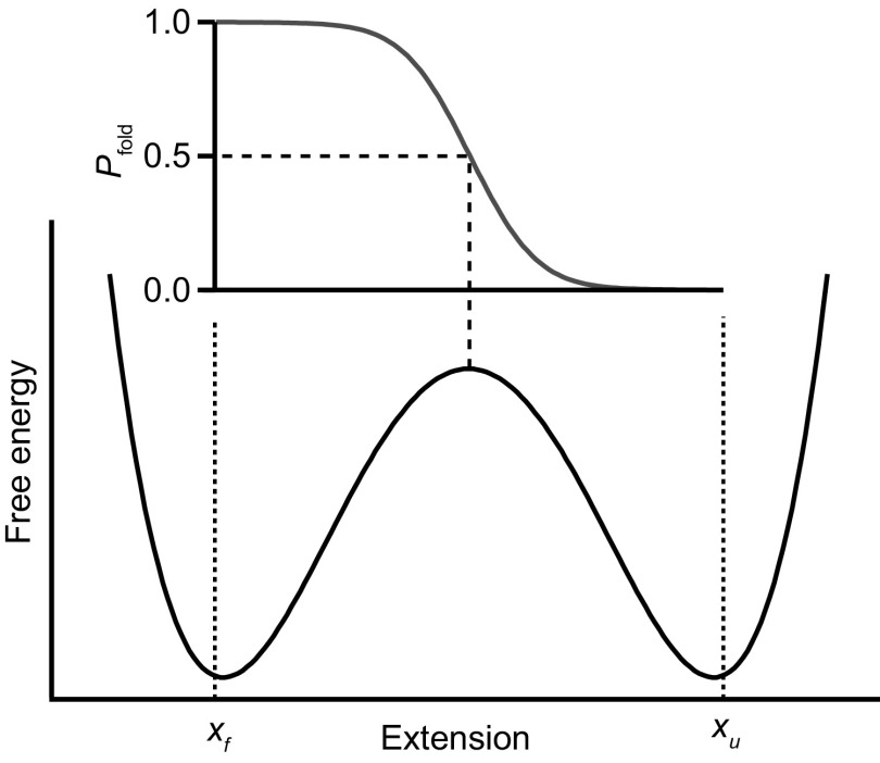
For a simple two-state system consisting of two potential wells separated by a barrier (Fig. 1), p_fold(x) is ∼0 when the molecule is in the unfolded state, ∼1 when it is in the folded state, and ∼1/2 when the molecule is at the top of the barrier (x = x^‡). Empirically, p_fold can be estimated from a measured trajectory of finite duration T for a given value of the reaction coordinate, x₀:

$$p_{\text{fold}}\left(x_0\right)={\displaystyle \underset{0}{\overset{T}{\int }}\delta (x_0-x\left(t\right))c_{x_f}\left(t\right)dt}/{\displaystyle \underset{0}{\overset{T}{\int }}\delta (x_0-x\left(t\right))dt},$$ [1]

where the function c(t) is 0 unless, subsequent to time t, the trajectory reaches an absorbing boundary at x_f (representing the location of the folded state along the reaction coordinate) before it hits a boundary at x_u (representing the location of the unfolded state), in which case c(t) = 1 (16). The denominator thus counts the number of times the trajectory crosses x₀, whereas the numerator counts the number of crossings where the trajectory subsequently reaches x_f before x_u.

Fig. 1.

Energy landscape and p_fold. Schematic energy landscape for a two-state system, with the corresponding splitting probability, p_fold(x), expected from Eq. 2. P_fold = 0.5 at the barrier. Dotted lines indicate the position of the absorbing boundaries.

Usually, p_fold(x) is used to test if the reaction coordinate is “good,” faithfully capturing the dynamics of the molecule during folding. At a minimum, for example, one should have p_fold ∼ 1/2 at the position along the reaction coordinate corresponding to the barrier in the energy landscape, x^‡ (with exact equality holding when diffusion is position-independent). However, p_fold(x) can also be related explicitly to the energy landscape for the folding. Assuming Langevin dynamics over a 1D profile G(x) with diffusion coefficient D, p_fold(x) is related to G(x) by (17, 18):

$$p_{\text{fold}}\left(x\right)={\displaystyle \underset{x}{\overset{x_u}{\int }}d{x}^{\prime }D{\left(x^{\prime }\right)}^{-1}{e}^{\beta G(x\prime )}}/{\displaystyle \underset{x_f}{\overset{x_u}{\int }}d{x}^{\prime }D{\left(x^{\prime }\right)}^{-1}{e}^{\beta G(x\prime )}}.$$ [2]

Here, β is the inverse thermal energy. Inversion of Eq. 2 then allows p_fold(x) estimates obtained from the trajectory to be used to reconstruct G(x): to within a constant,

$$G\left(x\right)={\beta }^{-1}\ln \left(-D\left(x\right)\frac{d{p}_{\text{fold}}}{dx}\right).$$ [3]

D generally varies with x in a manner that depends on the projection of the free-energy hypersurface onto the reaction coordinate (18); typically, D(x) is higher in the unfolded state and drops as the transition state is neared (19–21). However, it is often approximated as being constant (16), an approximation that is appropriate for hairpin folding, given previous work showing good agreement between measured rates and kinetic models with constant D (22), in which case Eqs. 2 and 3 become independent of D. Intriguingly, Eq. 2 is effectively the same as the equation relating the extension distributions in equilibrium and nonequilibrium regimes, as developed for reconstructing landscapes from force-jump measurements (7, 8). This earlier approach may therefore share some of the advantages of the p_fold approach, although its sensitivity to instrumental compliance has not yet been tested experimentally.

To test the application of p_fold(x) for landscape reconstructions, we used high-resolution measurements of the folding of individual two-state DNA hairpins under tension in optical traps, as described previously (15). Briefly, DNA constructs consisting of the desired hairpin sequence flanked by dsDNA handles were attached specifically to polystyrene beads to create “dumbbells” held in independently controlled optical traps (Fig. 2A, Upper Inset). Force was applied to induce the hairpin to fluctuate in equilibrium between folded and unfolded states, and the molecular extension was then measured over time. A typical extension record for the hairpin 30R50/T4 (15) (Fig. 2A, Left Inset), held at constant force just above F_1/2 (the force at which equal time is spent in each state) using a passive force clamp (23), is shown in Fig. 2A.

Fig. 2.

P_fold and energy landscape for a two-state DNA hairpin. (A) Extension of a single molecule of hairpin 30R50/T4 held under constant tension between two optical traps (Upper Inset) measured as the hairpin fluctuates between folded and unfolded states. Dashed lines indicate the absorbing boundaries for p_fold calculations. (Right Inset) Distribution of hairpin extension. (Left Inset) Hairpin sequence (light blue = T, dark blue = A, light red = C, dark red = G). (B) Splitting probability calculated from the trajectory (black) does not agree well with the splitting probability calculated from the apparent PMF implied by the extension distribution (blue), but it is very similar to the splitting probability found from the PMF after deconvolution of the instrument compliance (red). (C) PMF implied by the extension distribution (blue) and after deconvolution of the instrumental compliance (red).

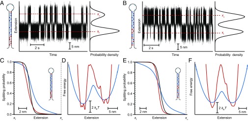
The splitting probability was first calculated directly from the trajectories (hereafter, this probability is denoted as p_traj) using Eq. 1, with the result shown in Fig. 2B (black). For comparison, we used the hairpin extension distribution, P(x) (Fig. 2A, Right Inset), to calculate the apparent potential of mean force (PMF) as −k_BTlnP(x) (Fig. 2C, blue), and then derived the splitting probability implied by the apparent PMF, hereafter denoted p_PMF(x), from Eq. 2. The result (Fig. 2B, blue) does not agree particularly well with p_traj(x): The apparent barrier location (where P = 1/2) differs by ∼2 nm between the two curves, and there are significant differences in the shape of the splitting probabilities as a function of x. A similar analysis was applied to extension trajectories of two other hairpins, 20TS06/T4 (Fig. 3A, Left Inset) and 20TS10/T4 (Fig. 3B, Left Inset), from a study by Woodside et al. (4). Again, p_traj(x) (Fig. 3 C and E, black), calculated directly from the trajectories (Fig. 3 A and B), did not agree particularly well with p_PMF(x) (Fig. 3 C and E, blue), calculated from the apparent PMFs (Fig. 3 D and F, blue).

Fig. 3.

P_fold and energy landscape for different DNA hairpin sequences. (A) Extension of hairpin 20TS06/T4 fluctuating between folded and unfolded states. Dashed lines indicate the absorbing boundaries for p_fold calculations. (Right Inset) Hairpin extension distribution. (Left Inset) Hairpin sequence. (B) Same for hairpin 20TS10/T4. (C) Splitting probabilities for hairpin 20TS06/T4 calculated from the trajectory (black), the apparent PMF implied by the extension distribution (blue), and the PMF after deconvolution (red). (E) Same for hairpin 20TS10/T4. (D) Apparent PMF implied by the extension distribution (blue) and PMF after deconvolution (red) for hairpin 20TS06/T4. (F) Same for hairpin 20TS10/T4.

Such disagreement has been interpreted previously as evidence that x is not a particularly good reaction coordinate for the hairpin folding (16). However, this analysis failed to consider how the compliance of the trapped dumbbells alters the apparent PMF (4) in a way that would invalidate direct comparison of p_PMF(x) and p_traj(x). In contrast, alternate analyses of the quality of the reaction coordinate based on a tensegrity parameter (24) and the conditional transition path probability (25) found that x was indeed a reasonable reaction coordinate for these hairpins. To demonstrate that instrumental effects were responsible for the disagreement between p_PMF(x) and p_traj(x), we recalculated p_PMF(x), this time using the landscapes reconstructed from the extension probabilities after removing the effects of the dumbbell compliance via deconvolution (4) (red curves in Fig. 2C and Fig. 3 D and F). In this case, the landscape-derived splitting probabilities (red curves in Fig. 2B and Fig. 3 C and E) agreed much better with the trajectory-derived probabilities all along the reaction coordinate, with the location of P = 1/2 differing by less than 1 nm for each hairpin, confirming that the end-to-end extension is a good reaction coordinate in these measurements.

Finally, we used p_traj(x) to recover G(x) from Eq. 3 for each of the three hairpins in the constant-D approximation. The results (Fig. 4, black) agreed well with the landscapes reconstructed for each hairpin by inverse Boltzmann transform from the deconvolved extension distributions (Fig. 4, red) but disagreed with the apparent PMFs found before deconvolution (blue curves in Fig. 2C and Fig. 3 D and F). We note that, of course, the landscape can only be reconstructed in this way between the absorbing boundaries x_f and x_u, but this region is the critical region for folding because it contains the barrier.

Fig. 4.

Energy landscapes reconstructed from p_traj. (A) Landscape reconstructed from p_traj (black) for hairpin 30R50/T4 agrees well with the landscape reconstructed from the deconvolved extension distribution (red), recovering the same barrier height and position. Good agreement is also found for hairpin 20TS06/T4 (B) and hairpin 20TS10/T4 (C).

Discussion

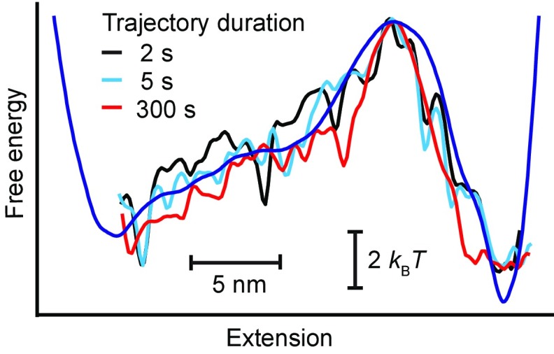
As seen in Fig. 4, the essential features, such as the height and position of the barrier, were captured in the landscapes reconstructed from Eq. 3, agreeing with the landscapes reconstructed from the deconvolved extension distributions within 1 k_BT or less for the barrier height and 1 nm for the position. Even such subtle features as the inflection in the 30R50/T4 landscape between the folded state and the barrier were recovered. The splitting probability thus allows free-energy landscapes to be recovered without the need to remove directly the effects of the probe compliance on the measurement. Notably, landscape reconstructions can be obtained from measurements containing remarkably few transitions [as few as 10 can provide a reasonable reconstruction (Fig. S1), compared with the hundreds or thousands required for other methods (4, 9, 11)], reducing the exceptionally low levels of instrumental noise and drift typically required for successful landscape reconstructions.

Fig. S1.

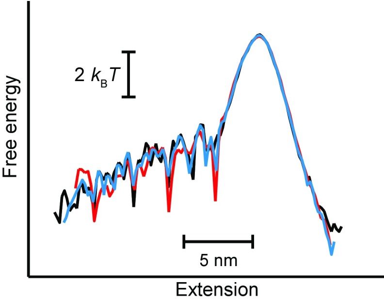
Landscape reconstructions using different trajectory durations. The landscapes recovered using Eq. 3 from the first 2 s (black) and 5 s (cyan) of the full trajectory for hairpin 30R50/T4 both agree quite well with the landscape recovered from the full 300-s trajectory (red), as well as with the landscape reconstructed from the deconvolved extension distribution (blue). The 2-s trajectory contains only six transitions (three each, folding and unfolding), and the 5-s trajectory contains only 14 transitions (seven each, folding and unfolding), demonstrating that very few trajectories are required to recover the correct barrier height and position.

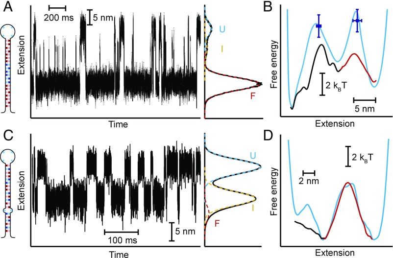
This approach can also be extended to multistate folders. A three-state hairpin (Fig. 5A) designed to fold sequentially in two steps (26, 27) was analyzed by calculating p_traj(x) independently for each transition in the folding pathway. The full landscape profile was then recovered piecewise by joining together the results from Eq. 2 for the two transitions (Fig. 5B, red and black). The positions of the two barriers agreed well with the results obtained from the force dependence of the kinetics (26) using the Bell–Zhurkov model (28) (Fig. 5B, blue), as well as with the barrier positions predicted by a model for the energy landscape of a hairpin under tension (15) (Fig. 5B, cyan). However, the results revealed one of the practical limitations of the method: the need for distinct states to be sufficiently well-resolved along the reaction coordinate so that the distributions of extensions from different states do not overlap significantly. In this case, overlap between the intermediate and unfolded states resulted in a barrier height (Fig. 5B, red) that was only half of the value expected from the force dependence of the kinetics and landscape model.

Fig. 5.

Landscape reconstruction for three-state hairpins. (A) Extension trajectory for a hairpin with a short-lived intermediate state. (Right Inset) Distribution of hairpin extensions shows significant overlap between the intermediate (I) and unfolded (U) states. (Left Inset) Hairpin sequence. (B) Landscape reconstructed from p_fold recovers the barrier positions expected from the force dependence of the kinetics and a model of the hairpin landscape, but significantly underestimates the height of the barrier between I and U. (C) Extension trajectory for a hairpin with a single-base mismatch. (Right Inset) Distribution of hairpin extensions shows significant overlap between the folded (F) and I states. (Left Inset) Hairpin sequence. (D) Landscape reconstructed from p_fold agrees well with the landscape found from the deconvolved extension distribution in the region of the barrier between I and U, but the barrier between F and I cannot be recovered from p_fold owing to the overlap of these states.

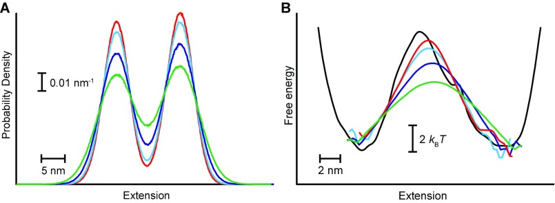
In the case of another three-state hairpin, this time containing a base pair mismatch (4), the overlap between the folded and intermediate states was sufficiently large (Fig. 5C, red and yellow) that the absorbing boundaries supposedly representing these two states when calculating p_traj(x) did not, in fact, discriminate between them. As a result, no barrier could be recovered from the p_fold analysis for this transition (Fig. 5D, black), even though the landscape between the intermediate and unfolded states recovered from Eq. 3 (Fig. 5D, red) agreed well with the profile reconstructed from the inverse Boltzmann transform of the deconvolved equilibrium extension distribution (4) (Fig. 5D, cyan). This effect of overlap between states was confirmed by adding a variable amount of Gaussian noise to the extension trajectory of a two-state hairpin, causing the tails of the distributions for the two states to overlap more extensively (Fig. S2A). Recalculating p_traj(x) in the presence of the additional noise, the height of the barrier in the landscape reconstructed via Eq. 3 was found to decrease continuously as the amount of overlap between the two states became ever more significant (Fig. S2B).

Fig. S2.

Effect of added noise on landscape reconstruction. (A) Adding Gaussian noise to the trajectory for hairpin 20TS10/T4 broadens the widths of the peaks corresponding to the folded and unfolded states, causing them increasingly to overlap (red: no added noise; cyan: 1 nm of noise; blue: 2 nm of noise; green: 3 nm of noise). (B) Increasing overlap between the states owing to increasing noise causes the apparent height of the barrier (red: no added noise; cyan: 1 nm of noise; blue: 2 nm of noise; green: 3 nm of noise) to decrease compared with the barrier in the landscape reconstructed from the deconvolved extension distribution (black).

Why are the landscape profiles found from p_fold(x) not affected as strongly by the mechanical properties of the force probe as in other landscape reconstruction methods based on force spectroscopy measurements (3)? We can understand this question by considering the difference between the motion of the molecule, the object of our true interest, and the motion of the beads, as actually observed. P_fold(x) is designed to capture the “decision” of the molecule to fold/unfold and cause a structural transition. This decision is driven primarily by the properties of the molecule’s intrinsic energy landscape; once the molecule has folded/unfolded, the decision is relayed to the beads via the compliant handles. Hence, the primary effect of the compliant tethers [at least for tethers that are not too rigid (29, 30)] is to add additional fluctuations on top of those fluctuations that arise from the molecular dynamics. With methods based on the distribution of extensions such as the inverse Boltzmann transform, the landscape reconstruction is degraded when the compliance fluctuations start to redistribute statistical weight from the folded/unfolded states to the barrier region, which is otherwise rarely occupied (i.e., when the tails of the folded/unfolded state distributions reach the barrier). Qualitatively, this degradation should occur when σ_k = (k_BT/k)^1/2 is comparable to Δx^‡, the distance to the barrier, where k is the effective stiffness of the system. The landscape reconstruction from p_fold, however, depends on the rate at which p_fold changes. Because most of the change in p_fold normally occurs across the barrier region, the reconstruction will only become degraded once the fluctuations from the folded or unfolded state reach all of the way across the barrier, significantly altering p_fold in the regions where it is close to constant. Because this distance is always larger than Δx^‡, the reconstruction based on p_fold is more robust against the added fluctuations from the instrumental compliance, even though the compliance of the traps and tethers still alters the distribution of the observed bead positions (and thus the extension of the molecule), as well as the time course of the transitions between states (13). It is not completely insensitive, however, starting to fail when there is too much overlap between the distributions for different states (as in Fig. 5). A full theoretical treatment of the problem, analogous to the theory for deconvolution of instrumental effects on the inverse Boltzmann transform (12), awaits future developments in theory.

To illustrate more directly the effects of changing the system compliance, we analyzed computational simulations of a molecule connected via a compliant tether (stiffness ranging from 1 to 0.1 pN/nm) to a probe applying a constant force (Fig. 6A), where the folding/unfolding involved diffusion across a model 1D potential chosen to be similar to the landscape for hairpin 30R50/T4. For the stiffest tether, the splitting probabilities calculated from the apparent PMF (Fig. 6B, dashed black line) and the extension trajectory (Fig. 6B, solid red line) are very similar, whereas for a more compliant tether (k = 0.6 pN/nm), p_PMF(x) (Fig. 6B, dashed brown line) diverges from p_traj(x) (Fig. 6B, solid brown line) in a manner similar to what is seen for the experimental hairpin data (Fig. 2B). This divergence becomes even more pronounced when the stiffness is lowered further, to 0.3 and 0.1 pN/nm (Fig. 6B, blue and green, respectively), because the apparent PMF becomes highly distorted by the effects of the compliance (Fig. 6C, dotted lines). Nevertheless, the results for p_traj(x) are effectively the same at the three highest stiffness values, and only diverge significantly at 0.1 pN/nm. The landscapes reconstructed via Eq. 3 thus agree reasonably well for the three highest stiffnesses (Fig. 6C, solid red, brown, and blue lines), demonstrating the relative insensitivity of the method to the system stiffness while recovering the shape of the 1D potential used in the simulations (Fig. 6C, black). In contrast, the landscapes derived from the inverse Boltzmann transform of the extension distribution (Fig. 6C, dotted lines) are affected much more strongly by the compliance at all stiffnesses below 1 pN/nm. These results agree with the qualitative criteria discussed above: Because x^‡ is just over 4 nm from the unfolded state, whereas the distance across the barrier is about 10 nm, we would expect to see compliance effects below k ∼1 pN/nm using the inverse Boltzmann transform (where σ_k ∼ Δx^‡), but these effects should become apparent using p_fold only at k ∼0.1 pN/nm.

Fig. 6.

Simulations of effect of tether stiffness on p_fold and landscape reconstruction. (A) Simulated extension trajectories (position of the bead) for a molecule diffusing across the 1D potential shown in C while connected by a compliant tether (black: k = 0.6 pN/nm; gray: k = 0.1 pN/nm) to a bead subjected to a constant force. (B) P_traj curves (solid lines) calculated from simulations at four stiffnesses (red: 1 pN/nm, brown: 0.6 pN/nm, blue: 0.3 pN/nm, green: 0.1 pN/nm) disagree with p_PMF curves from the same trajectories (dashed lines; black: 1 pN/nm) except at the highest stiffness (1 pN/nm). The p_traj curves are effectively the same for all except the lowest stiffness (0.1 pN/nm). (C) Landscapes reconstructed from p_traj (solid lines) are similar for all except the lowest tether stiffness and agree well with the 1D potential used in the simulation (black); only at 0.1 pN/nm (green) does the compliance significantly distort the reconstruction. In contrast, significant distortions are seen in the apparent PMF (dotted lines, offset for clarity) for all except the highest stiffness value.

We note that the success of this method for landscape reconstruction depends on the assumption that the experimental observable used to monitor the folding transitions (here, the end-to-end extension) provides a good reaction coordinate. If this assumption does not hold, the barrier reconstructed via p_fold may not describe the folding particularly well (31, 32). In the case of the hairpins studied here, the end-to-end extension has been proven to be a good reaction coordinate (25), which is quite reasonable because of the linear zippering mechanism for folding/unfolding under tension, but the same may not hold true for molecules folding by more complex mechanisms.

In conclusion, we have demonstrated a new approach for reconstructing energy landscapes from single-molecule trajectories using p_fold(x). P_fold(x) provides a more direct way of probing the barrier region in the folding landscape than other methods, avoiding the confounding effects introduced by the force probe and the need to remove them by error-prone deconvolution methods. With advantages that include simple calculation, the requirement for relatively few transitions, and no need to characterize carefully the properties of the force probe, the approach described here represents a powerful tool for studying energy landscapes.

Methods

Samples and Measurements.

DNA hairpin constructs consisting of hairpins of specific sequence connected to dsDNA handles were made and measured as described previously (4, 15). Briefly, hairpin constructs consisting of a single hairpin of the specified sequence connected at each end to dsDNA handles with a length of ∼600 bp and 1,000 bp were attached to polystyrene beads with a diameter of 600 nm and 820 nm held in a dual-trap system with a passive force clamp for measuring hairpin folding trajectories at constant force (23). The trap stiffness was 0.3 pN/nm. Data were sampled at 20–50 kHz during trajectories with a duration of 10–300 s at a given force and filtered at the Nyquist frequency.

Calculation of Splitting Probabilities.

P_traj(x) was calculated from trajectories with a duration of 10–300 s using Eq. 2 in MATLAB (MathWorks), with code provided courtesy of John Chodera, Memorial Sloan-Kettering Cancer Center, New York (16). The absorbing boundaries x_f and x_u, representing, respectively, the folded and unfolded states in a two-state transition, were chosen to be close to the center of the corresponding peaks in the extension distribution: x_f was placed ∼1 nm below the peak center for the folded state, whereas x_u was placed ∼1 nm above the peak center for the unfolded state. The result was insensitive to the exact location of x_f and x_u for physically reasonable choices (Fig. S3). For three-state hairpins, p_traj(x) was calculated sequentially for the folded-to-intermediate and intermediate-to-unfolded transitions. All calculations were done using steps in x of less than 0.2 nm.

Fig. S3.

Reconstruction is insensitive to the position of boundaries. Recalculating p_traj for different choices of the boundaries x_u and x_f (here, differing by ∼1 nm) did not materially change the shape of the reconstructed landscape.

Landscape Reconstructions.

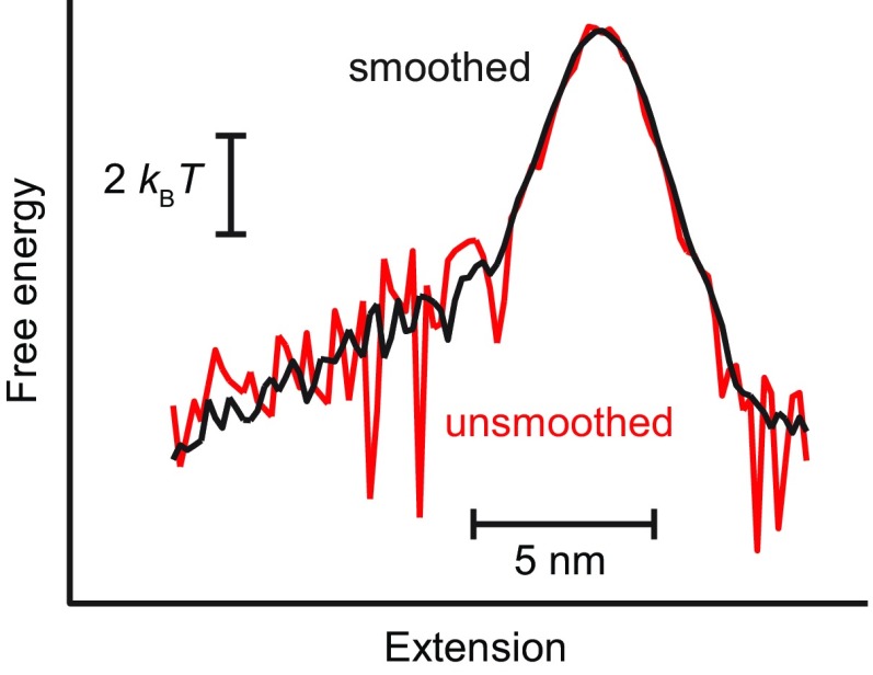
The landscape G(x) was calculated from p_traj(x) using Eq. 3, with D constant, after first smoothing p_traj(x) in a 1-nm window with a boxcar filter to reduce noise from differentiation. This filtering window was chosen to be smaller than the typical range over which substantial changes occur in the landscape but large enough to remove regions where fluctuations in p_traj produced a locally positive slope, such that the logarithm in Eq. 3 was undefined; the smoothing did not alter any of the central features of the landscape (Fig. S4). Differentiation was done numerically, using the central-difference method. Only the portion of the landscape between x_f and x_u was recovered this way, such that the potential wells were not fully reconstructed. Landscapes for multistate hairpins were reconstructed by joining together the reconstructions from each transition in the folding pathway. Landscape reconstructions done by inverse Boltzmann transform were performed as described previously (4). For the force-dependent kinetics analysis, microscopic transition rates (folding and unfolding) found from signal-pair correlation analysis (26) were fit to an exponential force dependence: k(F) = k₀exp(βF⋅Δx^‡), where Δx^‡ is the distance to the barrier and k₀ is the rate at zero force. Because the force range was insufficient to use more complete models for k(F) that include the barrier height (33), the latter was deduced from k₀ by assuming that the Kramers’ rate prefactor (34) was the same as the average for a panel of DNA hairpins measured previously (35) (∼5 × 10⁴ s⁻¹).

Fig. S4.

Effect of smoothing. Comparing the landscapes reconstructed from p_traj using Eq. 3, with (black) and without (red) smoothing, shows smoothing of p_traj does not affect the major features of the landscape.

Simulations.

Simulations were done as described previously (13). Briefly, diffusive motion over a defined 1D landscape similar to the diffusive motion for hairpin 30R50/T4 was assumed. The molecule was attached at one end to a bead of radius r and density ρ via a tether with stiffness k, and a constant force F was applied to the bead. Stochastic forces on the molecule and bead were drawn from Gaussian distributions of width (2γΔt/β)^1/2, where γ = 1/βD for the molecule (with diffusion coefficient D = 3 × 10⁵ nm²⋅s⁻¹) and γ = 6πηr (with viscosity η = 10⁻³ Pa⋅s⁻¹) for the bead, the time step Δt was 10⁻⁴ μs, r = 400 nm, and 1/β = 4.1 pN/nm. D for the molecule was chosen to be similar to the values found experimentally for DNA hairpin folding (35). The nonstochastic forces on the molecule and bead were, respectively, −V′(x₁) + k(x₂ − x₁) and k(x₁ − x₂) − Fx₂, where x₁ is the extension of the molecule, x₂ is the position of the bead, and V(x₁) is the potential landscape for the folding. A mixed simulation scheme was used, treating x₁ in pure Brownian fashion but evolving x₂ according to Langevin dynamics with explicit inertial terms using a modified Verlet-style algorithm (36). The density of the bead was ρ = 1.05 g/cm³ (as for polystyrene). The system was initially thermalized in a harmonic well matching the folded or unfolded well, and tested for correct energy equipartition and velocity autocorrelation decay. For each stiffness condition (k = 1, 0.6, 0.3, and 0.1 pN/nm), simulated data were collected for at least 80 s. Simulated data were analyzed in the same way as the experimental data.

References

- 1.Bryngelson JD, Wolynes PG. Spin glasses and the statistical mechanics of protein folding. Proc Natl Acad Sci USA. 1987;84(21):7524–7528. doi: 10.1073/pnas.84.21.7524. [DOI] [PMC free article] [PubMed] [Google Scholar]
- 2.Dill KA, MacCallum JL. The protein-folding problem, 50 years on. Science. 2012;338(6110):1042–1046. doi: 10.1126/science.1219021. [DOI] [PubMed] [Google Scholar]
- 3.Woodside MT, Block SM. Reconstructing folding energy landscapes by single-molecule force spectroscopy. Annu Rev Biophys. 2014;43:19–39. doi: 10.1146/annurev-biophys-051013-022754. [DOI] [PMC free article] [PubMed] [Google Scholar]
- 4.Woodside MT, et al. Direct measurement of the full, sequence-dependent folding landscape of a nucleic acid. Science. 2006;314(5801):1001–1004. doi: 10.1126/science.1133601. [DOI] [PMC free article] [PubMed] [Google Scholar]
- 5.Gebhardt JCM, Bornschlögl T, Rief M. Full distance-resolved folding energy landscape of one single protein molecule. Proc Natl Acad Sci USA. 2010;107(5):2013–2018. doi: 10.1073/pnas.0909854107. [DOI] [PMC free article] [PubMed] [Google Scholar]
- 6.de Messieres M, Brawn-Cinani B, La Porta A. Measuring the folding landscape of a harmonically constrained biopolymer. Biophys J. 2011;100(11):2736–2744. doi: 10.1016/j.bpj.2011.03.067. [DOI] [PMC free article] [PubMed] [Google Scholar]
- 7.Zhang Q, Brujic J, Vanden-Eijnden E. Reconstructing free energy profiles from nonequilibrium relaxation trajectories. J Stat Phys. 2011;144(2):344–366. [Google Scholar]
- 8.Lannon H, Haghpanah JS, Montclare JK, Vanden-Eijnden E, Brujic J. Force-clamp experiments reveal the free-energy profile and diffusion coefficient of the collapse of protein molecules. Phys Rev Lett. 2013;110(12):128301. doi: 10.1103/PhysRevLett.110.128301. [DOI] [PubMed] [Google Scholar]
- 9.Hummer G, Szabo A. Free energy reconstruction from nonequilibrium single-molecule pulling experiments. Proc Natl Acad Sci USA. 2001;98(7):3658–3661. doi: 10.1073/pnas.071034098. [DOI] [PMC free article] [PubMed] [Google Scholar]
- 10.Hummer G, Szabo A. Free energy profiles from single-molecule pulling experiments. Proc Natl Acad Sci USA. 2010;107(50):21441–21446. doi: 10.1073/pnas.1015661107. [DOI] [PMC free article] [PubMed] [Google Scholar]
- 11.Gupta AN, et al. Experimental validation of free-energy-landscape reconstruction from non-equilibrium single-molecule force spectroscopy measurements. Nat Phys. 2011;7(8):631–634. [Google Scholar]
- 12.Hinczewski M, Gebhardt JCM, Rief M, Thirumalai D. From mechanical folding trajectories to intrinsic energy landscapes of biopolymers. Proc Natl Acad Sci USA. 2013;110(12):4500–4505. doi: 10.1073/pnas.1214051110. [DOI] [PMC free article] [PubMed] [Google Scholar]
- 13.Woodside MT, Lambert J, Beach KSD. Determining intrachain diffusion coefficients for biopolymer dynamics from single-molecule force spectroscopy measurements. Biophys J. 2014;107(7):1647–1653. doi: 10.1016/j.bpj.2014.08.007. [DOI] [PMC free article] [PubMed] [Google Scholar]
- 14.Du R, Pande VS, Grosberg AY, Tanaka T, Shakhnovich ES. On the transition coordinate for protein folding. J Chem Phys. 1998;108(1):334–350. [Google Scholar]
- 15.Woodside MT, et al. Nanomechanical measurements of the sequence-dependent folding landscapes of single nucleic acid hairpins. Proc Natl Acad Sci USA. 2006;103(16):6190–6195. doi: 10.1073/pnas.0511048103. [DOI] [PMC free article] [PubMed] [Google Scholar]
- 16.Chodera JD, Pande VS. Splitting probabilities as a test of reaction coordinate choice in single-molecule experiments. Phys Rev Lett. 2011;107(9):098102. doi: 10.1103/PhysRevLett.107.098102. [DOI] [PMC free article] [PubMed] [Google Scholar]
- 17.Rhee YM, Pande VS. One-dimensional reaction coordinate and the corresponding potential of mean force from commitment probability distribution. J Phys Chem B. 2005;109(14):6780–6786. doi: 10.1021/jp045544s. [DOI] [PubMed] [Google Scholar]
- 18.Best RB, Hummer G. Coordinate-dependent diffusion in protein folding. Proc Natl Acad Sci USA. 2010;107(3):1088–1093. doi: 10.1073/pnas.0910390107. [DOI] [PMC free article] [PubMed] [Google Scholar]
- 19.Nettels D, Gopich IV, Hoffmann A, Schuler B. Ultrafast dynamics of protein collapse from single-molecule photon statistics. Proc Natl Acad Sci USA. 2007;104(8):2655–2660. doi: 10.1073/pnas.0611093104. [DOI] [PMC free article] [PubMed] [Google Scholar]
- 20.Kubelka J, Henry ER, Cellmer T, Hofrichter J, Eaton WA. Chemical, physical, and theoretical kinetics of an ultrafast folding protein. Proc Natl Acad Sci USA. 2008;105(48):18655–18662. doi: 10.1073/pnas.0808600105. [DOI] [PMC free article] [PubMed] [Google Scholar]
- 21.Soranno A, et al. Quantifying internal friction in unfolded and intrinsically disordered proteins with single-molecule spectroscopy. Proc Natl Acad Sci USA. 2012;109(44):17800–17806. doi: 10.1073/pnas.1117368109. [DOI] [PMC free article] [PubMed] [Google Scholar]
- 22.Manosas M, Collin D, Ritort F. Force-dependent fragility in RNA hairpins. Phys Rev Lett. 2006;96(21):218301. doi: 10.1103/PhysRevLett.96.218301. [DOI] [PubMed] [Google Scholar]
- 23.Greenleaf WJ, Woodside MT, Abbondanzieri EA, Block SM. Passive all-optical force clamp for high-resolution laser trapping. Phys Rev Lett. 2005;95(20):208102. doi: 10.1103/PhysRevLett.95.208102. [DOI] [PMC free article] [PubMed] [Google Scholar]
- 24.Morrison G, Hyeon C, Hinczewski M, Thirumalai D. Compaction and tensile forces determine the accuracy of folding landscape parameters from single molecule pulling experiments. Phys Rev Lett. 2011;106(13):138102. doi: 10.1103/PhysRevLett.106.138102. [DOI] [PMC free article] [PubMed] [Google Scholar]
- 25.Neupane K, Manuel AP, Lambert J, Woodside MT. Transition-path probability as a test of reaction-coordinate quality reveals DNA hairpin folding is a one-dimensional diffusive process. J Phys Chem Lett. 2015;6(6):1005–1010. doi: 10.1021/acs.jpclett.5b00176. [DOI] [PubMed] [Google Scholar]
- 26.Hoffmann A, Woodside MT. Signal-pair correlation analysis of single-molecule trajectories. Angew Chem Int Ed Engl. 2011;50(52):12643–12646. doi: 10.1002/anie.201104033. [DOI] [PubMed] [Google Scholar]
- 27.Woodside MT, García-García C, Block SM. Folding and unfolding single RNA molecules under tension. Curr Opin Chem Biol. 2008;12(6):640–646. doi: 10.1016/j.cbpa.2008.08.011. [DOI] [PMC free article] [PubMed] [Google Scholar]
- 28.Bell GI. Models for the specific adhesion of cells to cells. Science. 1978;200(4342):618–627. doi: 10.1126/science.347575. [DOI] [PubMed] [Google Scholar]
- 29.Chang J-C, de Messieres M, La Porta A. Effect of handle length and microsphere size on transition kinetics in single-molecule experiments. Phys Rev E Stat Nonlin Soft Matter Phys. 2013;87(1):012721. doi: 10.1103/PhysRevE.87.012721. [DOI] [PubMed] [Google Scholar]
- 30.Makarov DE. Communication: Does force spectroscopy of biomolecules probe their intrinsic dynamic properties? J Chem Phys. 2014;141(24):241103. doi: 10.1063/1.4904895. [DOI] [PubMed] [Google Scholar]
- 31.Dudko OK, Graham TGW, Best RB. Locating the barrier for folding of single molecules under an external force. Phys Rev Lett. 2011;107(20):208301. doi: 10.1103/PhysRevLett.107.208301. [DOI] [PubMed] [Google Scholar]
- 32.Best RB, Hummer G. Reaction coordinates and rates from transition paths. Proc Natl Acad Sci USA. 2005;102(19):6732–6737. doi: 10.1073/pnas.0408098102. [DOI] [PMC free article] [PubMed] [Google Scholar]
- 33.Dudko OK, Hummer G, Szabo A. Theory, analysis, and interpretation of single-molecule force spectroscopy experiments. Proc Natl Acad Sci USA. 2008;105(41):15755–15760. doi: 10.1073/pnas.0806085105. [DOI] [PMC free article] [PubMed] [Google Scholar]
- 34.Hanggi P, Talkner P, Borkovec M. Reaction-rate theory—50 years after Kramers. Rev Mod Phys. 1990;62(2):251–341. [Google Scholar]
- 35.Neupane K, et al. Transition path times for nucleic Acid folding determined from energy-landscape analysis of single-molecule trajectories. Phys Rev Lett. 2012;109(6):068102. doi: 10.1103/PhysRevLett.109.068102. [DOI] [PubMed] [Google Scholar]
- 36.Gronbech-Jensen N, Farago O. A simple and effective Verlet-type algorithm for simulating Langevin dynamics. Mol Phys. 2013;111(8):983–991. [Google Scholar]