Recursion-Transform method to a non-regular m×n cobweb with an arbitrary longitude

Abstract

A general Recursion-Transform method is put forward and is applied to resolving a difficult problem of the two-point resistance in a non-regular m × n cobweb network with an arbitrary longitude (or call radial), which has never been solved before as the Green’s function technique and the Laplacian matrix approach are difficult in this case. Looking for the explicit solutions of non-regular lattices is important but difficult, since the non-regular condition is like a wall or trap which affects the behavior of finite network. This paper gives several general formulae of the resistance between any two nodes in a non-regular cobweb network in both finite and infinite cases by the R-T method which, is mainly composed of the characteristic roots, is simpler and can be easier to use in practice. As applications, several interesting results are deduced from a general formula, and a globe network is generalized.

The computation of the two-point resistance in a resistor network is a classical problem in circuit theory and graph theory, which has been researched for more than 160 years. The computation of resistance is relevant to a wide range of problems ranging from classical transport in disordered media¹, first-passage processes², lattice Greens functions³,⁴, random walks⁵, resistance distance⁶,⁷, to graph theory⁴,⁸. However, it is usually very difficult to obtain the explicit expression of resistance in a non-regular resistor networks (it means different resistors are arranged on the network, which differs from a normal resistor network), since the non-regular condition is like a wall or trap which affects the behavior of finite network. Thus the construction of and research on the models of non-regular networks therefore make sense for theories and applications.

There may be more calculation methods of equivalent resistance of a resistor network, but the main research methods which can calculate the equivalent resistance of an m × n resistor networks are only a few. For example, the first method is that Kirchhoff found the node current law (KCL) and the circuit voltage law (KVL) in 1845, in theory the methods can resolve all the problems but that is not the case because of the algebra and technique; The second method is that Cserti evaluated the two-point resistance using the lattice Green’s function⁹, his study is mainly confined to regular lattices of infinite size; The third method is Ref. 10,11 formulated a different approach (call the Laplacian matrix method), especially Ref. 11 derived the explicit expressions for the two-point resistance in arbitrary finite and infinite lattices with normative boundary (such as free, periodic boundary etc.) in terms of the eigenvalues and eigenvectors of the Laplacian matrix relies on two matrices along two vertical directions. After some improvements, the Laplacian approach has been extended to the complex impedance network¹² and to the resistor network with zero resistor boundary¹³,¹⁴,¹⁵; The fourth method is that Tan created the Recursion-Transform (R-T) method¹⁶ (one may refer Ref. 17, 18, 19, 20, 21), which compute the equivalent resistance relies on just one matrix along one direction, and the explicit resistance is expressed by a single summation¹⁷,¹⁸,¹⁹,²⁰,²¹. The advantage of the R-T method is different from the Laplacian matrix method is that it only dependent on a matrix not two matrices. Very recently Ref. 22 propose a method of nodal potentials which may be able to calculate all kinds of resistor networks, but we find it is difficult to obtain the concise expression of resistance of an arbitrary m × n resistor networks except for a series of simple resistor networks (perhaps this method will also lead to solving this problem in the future).

For the arbitrary resistor networks of various topologies, various new results of the resistor networks have been obtained by applying the R-T method. For example, a cobweb model¹⁷, a globe network¹⁸, a fan network¹⁹, a cobweb network with 2r boundary²⁰, a hammock network¹⁵, especially, very recently this method was further generalized in Ref. 21, which can applied to the resistor network with an arbitrary boundary.

However, there are still some non-regular resistor networks unresolved because of the complexity of the boundary conditions of the network in real life. Thanks to the R-T method provides us with new technique to deal with the complex networks of various topologies. In this paper we will study the resistances of a complex network with arbitrary resistors on the longitude line.

Figure. 1 is called a non-regular m × n resistor cobweb which has arbitrary resistor r₂ on the boundary and an arbitrary longitude with arbitrary resistors r₁ (in order to facilitate our study, we refer the name in globe and call the radial as longitude, and call the circle line as latitude). This paper focus on the computation of the two-point resistance between any two nodes in the non-regular m × n cobweb network, which has never been solved before, the Green’s function technique and the Laplacian matrix approach are difficult in this case because they depend on the two matrices along two directions (one may refer the discussion at the end). Figure. 1 is a multipurpose network model, when the boundary resistor r₂ = 0, the non-regular cobweb degrades into a nearly globe network as shown in Fig. 2.

Figure 1. A non-regular 7 × 14 cobweb with arbitrary top boundary and an arbitrary longitude (with r₁), which has 7 latitudes (including boundary) and 14 longitudes.

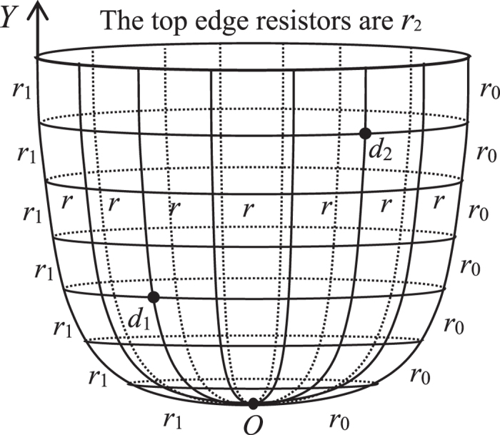
Bonds in the longitudes and latitudes directions represent, respectively, resistors r₀ and r except for the resistor r₁ on a longitude and the boundary resistor r₂.

Figure 2. An 7 × 12 globe network with an arbitrary longitude, which has 7 latitude and 12 longitude.

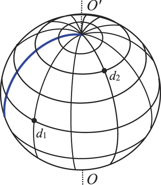
Bonds in the longitudes and latitudes directions represent, respectively, resistors r₀ and r except for an arbitrary longitude.

Results

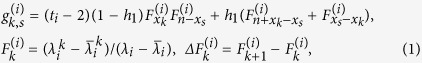
The boundary resistor r₂ is a key parameter since the different parameter can represent different geometric structure, such as a globe is from a nearly cobweb with r₂ = 0. In this paper we will consider three cases of r₂ = {0, r, 2r}, and give several results in three cases. We first define several variables , , S_k,i and t_i for later uses by

where , and are for later uses expressed as

Noticing that θ_i has three kinds different values with three different resistors of r₂ = {0, r, 2r}

The results in the case of r ₂ = r

Consider a nearly m × n resistor cobweb with resistances r and r₀ in the respective latitudes and longitudes except for a longitude resistors r₁, where m and n are, respectively, the numbers of grids along longitude and latitude directions as shown in Fig. 1. Assuming the center node O is the origin of the rectangular coordinate system, and a longitude with r₁ act as Y axis. Denote nodes of the network by coordinate {x, y}. The equivalent resistance between any two nodes d₁(x₁, y₁) and d₂(x₂, y₂) in a nearly m × n cobweb network with free boundary can be written as

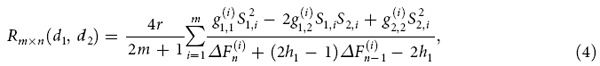where θ_i = (2i − 1)π/(2m + 1), , and h_k, S_k,i are respectively defined in (1) and (2)

In particular, from (4) we have the special cases:

Case 1

When h₁ = 1, the network degrades into a normal cobweb, we have

where Δx = x₂ − x₁.

Case 2

When h₁ = 0, we have

Case 3

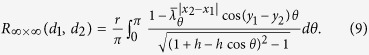
When n → ∞, x₁, x₂ → ∞ with x₁ − x₂ finite, we have

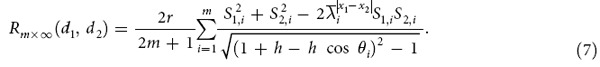Case 4

When x₁ = x₂ = x, m,n → ∞ with y₁, y₂ finite, we have

Case 5

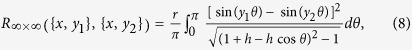
When m,n → ∞, but x₁ − x₂ and y₁ − y₂ are finite, we have

where .

Case 6

When d₁ = (x, y₁) and d₂ = (x, y₂) are both on the same longitude, we have

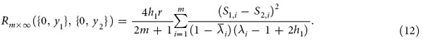
Especially, when d₁ = (0, y₁) and d₂ = (0, y₂) are both on the Y axis, we have

and when n → ∞ with y₁, y₂ finite, we have

The result in the case of r ₂ = 2r

When r₂ = 2r, the equivalent resistance between any two nodes d₁(x₁, y₁) and d₂(x₂, y₂) in a nearly m × n cobweb network with 2r boundary is

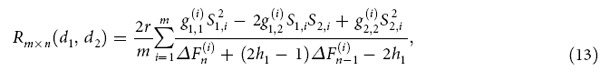where . Especially, when h₁ = 1, from (13) we have

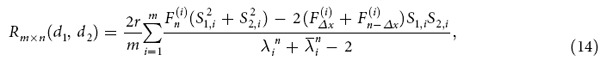with Δx = x₂ − x₁.

The result in the case of r ₂ = 0

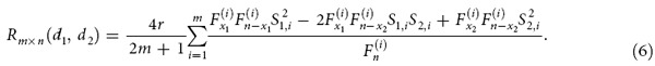
When r₂ = 0, the non-regular cobweb network degrades into a nearly globe network with an arbitrary longitude as shown in Fig. 2. The equivalent resistance between any two nodes d₁(x₁, y₁) and d₂(x₂, y₂) in a nearly m × n globe network with an arbitrary longitude can be written as

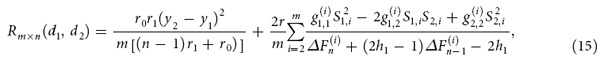where θ_k = (k − 1)π/m. Especially, when h₁ = 1, the nearly globe degrades into a normal globe network, from (15) we have

Note that: the above similar formulae are different because their θ_i are different from each other. The above results are original research which have not been solved before.

Method

Calculating resistance by Ohm’s law

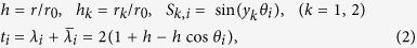
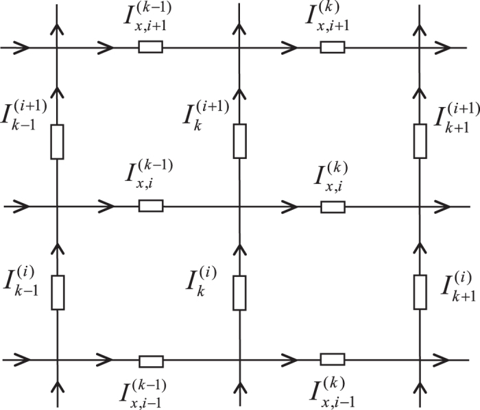
Assuming the electric current J is constant and goes from the input d₁(x₁, y₁) to the output d₂(x₂, y₂) as shown in Fig. 1. Denote the currents in all segments of the network as shown in Fig. 3. The resulting currents passing through all m row (latitude) resistors are: , , … (1 ≤ k ≤ m); the resulting currents passing through all n column (longitude) resistors are: , ,… (0 ≤ k ≤ n).

Figure 3. Segment of the cobweb with current parameters and directions.

To find the resistance , using Ohm’s law the potential difference may be measured along a path from d₁(x₁, y₁) to O and then to d₂(x₂, y₂), so we have

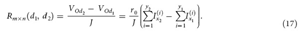How to resolve the current parameters and is the key to the problem. We are going to resolve the problem by the R-T approach.

Modeling the matrix equations

A segment of the rectangular network is shown in Fig. 3. Using Kirchhoff’s law to study the resistor network, the nodes current equations and the meshes voltage equations can be achieved from Fig. 3. We focus on the four rectangular meshes and nine nodes, this gives the matrix relation (one may refer ^{[17, 18, 19, 20, 21]})

where I_k and H_x are respectively m × 1 column matrix, and reads

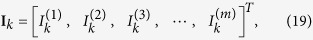where [ ]^T denote matrix transposes, and (H_k)_i is the elements of H_x with the injection of current J at d₁(x₁, y₁) and the exit of current J at d₂(x₂, y₂), and A_m is an m × m matrix,

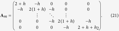where h = r/r₀, h₂ = r₂/r₀.

We consider the bound conditions of a specific longitude with resistors r₁. Applying Kirchhoff’s laws to two meshes adjacent to the specific longitude we obtain three matrix equations to model the bound currents,

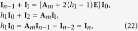where h₁ = r₁/r₀ and E is an m-dimensional identity matrix, and matrix A_m is given by (21).

Above Eqs.(18) ~ (22) are all equations we need to calculate the equivalent resistance of the non-regular m × n cobweb network with an arbitrary longitude.

Approach of the matrix transform

To solve the matrix equation (18) we rebuild a new difference equation and resolve Eq.(18) indirectly by means of matrix transform. First, the eigenvalues t_i (i = 1, 2,…,m) of A_m are the m solutions of the equation

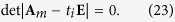Since A_m is a special tridiagonal matrix which is Hermitian, it can be diagonalized by a similarity transformation to yield

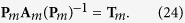where T_m = diag{t₁, t₂,…,t_m} is a diagonal matrix with eigenvalues t_i of A_m in the diagonal, and the column vectors of P_m is the eigenvector of A_m. From (23) and (24) we obtain (2) in the cases of r₂ = {0, r, 2r}, meanwhile, obtain , and , respectively, appeared in Eqs.(15), (4) and (13).

In order to implement the matrix transform, we define

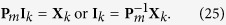where X_m is an m × 1 column matrix, and reads

Thus we apply P_m to (18) on the left-hand side, and obtain a new matrix equation

Assuming the row vectors of matrix P_m is

When r₂ = {0, r, 2r}, we can obtain the explicit matrix P_m. We let the i^th element of the column vector X_k be . Then (27) gives

where (reads as ζ_1,i , and as ζ_2,i)

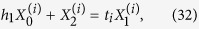
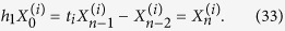
Supposing are the roots of the characteristic equation for , from (29) we obtain (3). Next we conduct the same matrix transform to (22), we are led to

When r₂ = {0, r, 2r}, from the above equations (29) ~ (33) we therefore obtain after some algebra and reduction the two solutions and needed in our resistance calculation (17).

Derivation of the resistance formula

According to Eq. (17), the key currents and must be calculated for deriving the equivalent resistance R_{m × n}(d₁, d₂). From (25) we have , thus we obtain and . Finally, substituting and into (17), we therefore obtain the resistance R_{m × n}(d₁, d₂) in three cases of r₂ = {0, r, 2r}.

Discussion

Considerable progress has recently been made in the development of techniques to exactly determine two-point resistances in the networks of various topologies. In this paper the R-T method is applied to computation of the two-point resistance in a non-regular m × n cobweb network with an arbitrary boundary and an arbitrary longitude, which has never been solved before. The resistance formulae are given in the form of a single summation, and several previous research results have become our special cases. Such as formula (5) is equivalent to the result of Ref. 19, formula (14) is the same with the result of Ref. 20, formula (16) agrees with the result of Ref. 18, and formula (9) is the same with the result of Ref. 21. Obviously, Fig. 1 is a multipurpose network model which contains several different cases.

The reason why the Green’s function technique and the Laplacian matrix approach are difficult to resolve the non-regular network in Fig. 1 is that they depend on the two matrices along two directions, besides matrix (21), there is another matrix with an arbitrary element of r₁ when we set up a matrix along the latitudes directions, which is impossible for us to obtain the explicit eigenvalues and eigenvectors of a matrix with arbitrary element.

The reason why we just consider r₂ = {0, r, 2r} is that, at present, we cannot obtain the explicit eigenvalues and eigenvectors of matrix (21) when r₂ ≠ {0, r, 2r}, although the R-T method is feasible. Of course, we can obtain the resistance of the non-regular network as soon as we obtain the explicit eigenvalues and eigenvectors of matrix (21).

The R-T method splits the derivation into three parts. The first creates a recursion relation between the current distributions on three successive longitude lines. The second part derives a recursion relation between the current distributions on the bound longitude. The third part implements the matrix transform of diagonalization to produce a recurrence relation involving only variables on the same axis. Basically, the method reduces the problem from two dimensions to one dimension.

In addition, an important usefulness is that the R-T method can be extended to impedance networks, since the Ohm’s law based on which the method is formulated is applicable to impedances. Such as the grid elements r and r₀ can be either a resistors or impedances, we can therefore study the m × n complex impedance networks by the R-T method.

Additional Information

How to cite this article: Tan, Z.-Z. Recursion-Transform method to a non-regular m×n cobweb with an arbitrary longitude. Sci. Rep. 5, 11266; doi: 10.1038/srep11266 (2015).

References

- Kirkpatrick S. Percolation & Conduction, Rev. Mod. Phys. 45, 574–588 (1973). [Google Scholar]
- Redner S. A Guide to First-Passage Processes Cambridge University Press, Cambridge, 2001. [Google Scholar]
- Katsura S. & Inawashiro S. Lattice Green’s functions for the rectangular and the square lattices at arbitrary points. J. Math. Phys. 12, 1622 (1971). [Google Scholar]
- Kook. Woong Combinatorial Green’s function of a graph and applications to networks, Advances in Applied Mathematics 46 (2011) 417–423 [Google Scholar]
- Doyle P. G. & Snell J. L. Random Walks and Electrical Networks, The Mathematical Association of America, Washington, DC, 1984. [Google Scholar]
- Klein D. J. & Randi M. Resistance distance, J. Math. Chem. 12, 8195 (1993). [Google Scholar]
- Xiao W. J. & Gutman I. Resistance distance and Laplacian spectrum, Theory Chem. Acc. 110, 284–289 (2003). [Google Scholar]
- Novak L. & Gibbons A. Hybrid Graph Theory and Network Analysis, Cambridge Univ. Press, 2009. [Google Scholar]
- Cserti J. Application of the lattice Green’s function for calculating the resistance of an infinite network of resistors. Am. J. Phys. 68, 896 (2000). [Google Scholar]
- Chandra A. K., Raghavan P., Ruzzo W. L., Smolensky R. & Tiwari P. “The electrical resistance of a graph captures its commute and cover times”, in Proceedings of the 21st Annnual ACM Symposium on the Theory of Computing (ACM Press, New York, 1989), pp. 574–586
- Wu F. Y. Theory of resistor networks: the two-point resistance. J. Phys. A: Math. Gen. 37, 6653 (2004). [Google Scholar]
- Tzeng W. J. & Wu F. Y. Theory of impedance networks: the two-point impedance and LC resonances. J. Phys. A: Math. Gen. 39, 8579 (2006). [Google Scholar]
- Izmailian N. Sh., Kenna R. & Wu F. Y. The two-point resistance of a resistor network: a new formulation and application to the cobweb network. J. Phys. A: Math. Theor. 47, 035003(2014). [Google Scholar]
- Izmailian N. Sh. & Kenna R. A generalised formulation of the Laplacian approach to resistor networks. J. Stat. Mech. 09, 1742–5468, P09016 (2014). [Google Scholar]
- Essam J. W., Izmailian N. Sh., Kenna R. & Tan Z. Z. Comparison of methods to determine point-to-point resistance in nearly rectangular networks with application to a “hammock” network. arXiv:1411.1916v1, (2014). [DOI] [PMC free article] [PubMed]
- Tan Z. Z. Resistance network Model. (Xidian Univ. Press, Xi’an 2011). [Google Scholar]
- Tan Z. Z., Zhou L. & Yang J. H. The equivalent resistance of a 3×n cobweb network and its conjecture of an m×n cobweb network. J. Phys. A: Math. Theor. 46, 195202 (2013). [Google Scholar]
- Tan Z. Z., Essam J. W. & Wu F. Y. Two-point resistance of a resistor network embedded on a globe. Phys. Rev. E. 90, 012130 (2014). [DOI] [PubMed] [Google Scholar]
- Essam J. W., Tan Z. Z. & Wu F. Y. Resistance between two nodes in general position on an m×n fan network. Phys. Rev. E. 90, 032130 (2014). [DOI] [PubMed] [Google Scholar]
- Tan Z. Z. & Fang J. H. Two-point resistance of a cobweb network with a 2r boundary. Commun. Theor. Phys. 63, 36–44 (2015). [Google Scholar]
- Tan Z. Z. Recursion-Rransform approach to compute the resistance of a resistor network with an arbitrary boundary. Chin. Phys. B. 24, 020503 (2015). [Google Scholar]
- Kagan. Mikhail On equivalent resistance of electrical circuits. Am. J. Phys. 83, 53 (2015). [Google Scholar]