Clustering-Induced Multi-task Learning for AD/MCI Classification

Abstract

In this work, we formulate a clustering-induced multi-task learning method for feature selection in Alzheimer’s Disease (AD) or Mild Cognitive Impairment (MCI) diagnosis. Unlike the previous methods that often assumed a unimodal data distribution, we take into account the underlying multipeak¹ distribution of classes. The rationale for our approach is that it is likely for neuroimaging data to have multiple peaks or modes in distribution due to the inter-subject variability. In this regard, we use a clustering method to discover the multipeak distributional characteristics and define subclasses based on the clustering results, in which each cluster covers a peak. We then encode the respective subclasses, i.e., clusters, with their unique codes by imposing the subclasses of the same original class close to each other and those of different original classes distinct from each other. We finally formulate a multi-task learning problem in an ℓ_2,1-penalized regression framework by taking the codes as new label vectors of our training samples, through which we select features for classification. In our experimental results on the ADNI dataset, we validated the effectiveness of the proposed method by achieving the maximal classification accuracies of 95.18% (AD/Normal Control: NC), 79.52% (MCI/NC), and 72.02% (MCI converter/MCI non-converter), outperforming the competing single-task learning method.

1 Introduction

From a computational modeling perspective, while the feature dimension of neuroimaging data is high in nature, we have a very limited number of observations/samples available. This so-called “small-n-large-p” problem has been of a great challenge in the field to build a robust model that can correctly identify a clinical label of a subject, e.g., AD, MCI, Normal Control (NC) [10]. For this reason, reducing the feature dimensionality, by which we can mitigate the overfitting problem and improve a model’s generalizability, has been considered as a prevalent step in building a computer-aided AD diagnosis system as well as neuroimaging analysis [6]. On the other hand, pathologically, since the disease-related atrophy or hypo-metabolism could happen in the part of a Region Of Interest (ROI), or cover small regions of multiple ROIs, it is difficult to predefine ROIs, and thus important to consider the whole brain features and then select the most informative ones for better diagnosis.

The main limitation of the previous methods of Principal Component Analysis (PCA) and Linear Discriminant Analysis (LDA), and an embedded method such as ℓ₁-penalized regression model is that they consider a single mapping or a single weight coefficient vector in reducing the dimensionality. But, if the underlying data distribution is not unimodal, e.g., mixture of Gaussians, then these methods would fail to find the proper mapping or weighting functions, and thus result in performance degradation. In this regard, Zhu and Martinez proposed a Subclass Discriminant Analysis (SDA) [12] that first clustered samples of each class and then reformulated the conventional LDA by regarding clusters as subclasses. Recently, Liao et al. applied the SDA method to segment prostate MR images and showed the effectiveness of the subclass-based approach [5].

In this paper, we propose a novel method of feature selection for AD/MCI diagnosis by integrating the embedded method with the subclass-based approach. The motivation of clustering samples per class is the potential heterogeneity within a group, which may result from (1) a wrong clinical diagnosis; (2) different sub-types in AD (e.g., amnestic/non-amnestic); (3) conversion of MCI non-converter or NC to AD after the follow-up time. Specifically, we first divide each class into multiple subclasses by means of clustering, with which we can approximate the inherent multipeak data distribution of a class. Note that we regard each cluster as a subclass by following Zhu and Martinez’s work [12]. Based on the clustering results, we encode the respective subclasses with their unique codes, for which we impose the subclasses of the same original class close to each other and those of different original classes distinct from each other. By setting the codes as new labels of our training samples, we finally formulate a multi-task learning problem in an ℓ_2,1-penalized regression framework that takes into account the multipeak data distributions, and thus help enhance the diagnostic performances.

2 Materials and Image Processing

We use the ADNI dataset publicly available on the web². Specifically, we consider only the baseline Magnetic Resonance Imaging (MRI) and 18-Fluoro-DeoxyGlucose (FDG) Positron Emission Tomography (PET) data acquired from 51 AD, 99 MCI, and 52 NC subjects. For the MCI subjects, they were further clinically subdivided into 43 MCI Converters (MCI-C) and 56 MCI Non-Converters (MCI-NC), who progressed and did not progress to AD in 18 months, respectively.

The MR images were preprocessed by applying the prevalent procedures of Anterior Commissure (AC)-Posterior Commissure (PC) correction, skull-stripping, and cerebellum removal. Specifically, we used MIPAV software³ for AC-PC correction, resampled images to 256×256×256, and applied N3 algorithm [8] for intensity inhomogeneity correction. Then, structural MR images were segmented into three tissue types of Gray Matter (GM), White Matter (WM) and CSF with FAST in FSL package⁴. We finally parcellated them into 93 ROIs by warping Kabani et al.’s atlas [4] to each subject’s brain space. Regarding FDG-PET images, they were rigidly aligned to the respective MR images, and then applied parcellation propagated from the atlas by registration. For each ROI, we used the GM⁵ tissue volume from MRI, and the mean intensity from FDG-PET as features. Therefore, we have 93 features from an MR image and the same dimensional features from an FDG-PET image.

3 Method

Throughout the paper, we denote matrices as boldface uppercase letters, vectors as boldface lowercase letters, and scalars as normal italic letters, respectively. For a matrix X = [x_ij], its i-th row and j-th column are denoted as xⁱ and x_j, respectively. We further denote the Frobenius norm and ℓ_2,1-norm of a matrix X as ${\Vert \mathbf{X}\Vert }_F=\sqrt{{\sum }_i{\Vert {\mathbf{x}}^i\Vert }_2^2}=\sqrt{{\sum }_j{\Vert {\mathbf{x}}_j\Vert }_2^2}$ and ${\Vert \mathbf{X}\Vert }_{2,1}={\sum }_i{\Vert {\mathbf{x}}^i\Vert }_2={\sum }_i\sqrt{{\sum }_j{x}_{ij}^2}$, respectively, and the ℓ₁-norm of a vector as ||w||₁ = Σ_i |w_i|.

3.1 Preliminaries

Let X ∈ R^N×D and y ∈ R^N denote, respectively, the D neuroimaging features and clinical labels of N samples. Assuming that the clinical label can be represented by a linear combination of the neuroimaging features, many research groups have utilized a least square regression model with various regularization terms. In particular, despite its simple form, the ℓ₁-penalized linear regression model has been widely and successfully used in the literature [1, 11], as formulated as follows:

$$\underset{\mathbf{w}}{min}{\Vert \mathbf{y}-\mathbf{Xw}\Vert }_2^2+{\lambda }_1{\Vert \mathbf{w}\Vert }_1$$ (1)

where λ₁ denotes a sparsity control parameter. Since this method finds a single optimal weight coefficient vector w that regresses the target response vector y, it is classified into a single-task learning (Fig. 1(a)) in machine learning.

Fig. 1.

In the response vector/matrix, the colors of blue, red, and white represent 1, −1, and 0, respectively. In multi-task learning, each row of the response matrix represents a newly defined sparse code for each sample by the proposed method.

If there exists additional class-related information, then we can further extend the ℓ₁-penalized linear regression model into a more sophisticated ℓ_2,1-penalized one as follows:

$$\underset{\mathbf{w}}{min}{\Vert \mathbf{Y}-\mathbf{XW}\Vert }_F^2+{\lambda }_2{\Vert \mathbf{W}\Vert }_{2,1}$$ (2)

where Y = [y₁, · · ·, y_S] ∈ R^N×S is a target response matrix, W = [w₁, · · ·, w_S] ∈ R^D×S is a weight coefficient matrix, S is the number of response variables, and λ₂ denotes a group sparsity control parameter. In machine learning, this framework is classified into a multi-task learning⁶ (Fig. 1(b)) because it needs to find a set of weight coefficient vectors by regressing multiple response values, simultaneously.

3.2 Clustering-Induced Multi-task Learning

Because of the inter-subject variability [3, 7], it is likely for neuroimaging data to have multiple peaks in distribution. In this paper, we argue that it is necessary to consider the underlying multipeak data distribution in feature selection. To this end, we propose to divide classes into subclasses and to utilize the resulting subclass information for guiding feature selection by means of a multi-task learning.

To divide the training samples of each original class into their respective subclasses, we exploit a clustering technique. Specifically, thanks to its simplicity and computational efficiency, especially in a high dimensional space, we use a K-means algorithm. Note that the resulting clusters are regarded as subclasses, following Zhu and Martinez’s work [12]. We then encode the subclasses with their unique labels, for which we use discriminative sparse codes to enhance classification performance. Let K₍₊₎ and K₍₋₎ denote, respectively, the number of clusters/subclasses for the original classes of ‘+’ and ‘−’. Without loss of generality, we define sparse codes for the subclasses of the original classes of ‘+’ and ‘−’ as follows:

$${\mathbf{s}}_l^{(+)}=\left[\begin{array}{ccc}+1& {\mathbf{z}}_l^{(+)}& {\mathbf{0}}_{K_{(-)}}\end{array}\right]$$ (3)

$${\mathbf{s}}_m^{(-)}=\left[\begin{array}{ccc}-1& {\mathbf{0}}_{K_{(+)}}& {\mathbf{z}}_m^{(-)}\end{array}\right]$$ (4)

where l ∈ {1, · · ·, K₍₊₎}, m ∈ {1, · · ·, K₍₋₎}, 0_K(+) and 0_K(−) denote, respectively, zero row vectors with K₍₊₎ and K₍₋₎ elements, and ${\mathbf{z}}_l^{(+)}\in {\{0,1\}}^{K_{(+)}}$ and ${\mathbf{z}}_m^{(-)}\in {\{0,-1\}}^{K_{(-)}}$ denote, respectively, indicator row vectors in which only the l-th/m-th element is set to 1/−1 and the others are 0. Thus, the full code set is defined as follows:

$$\mathbb{S}=\{{\mathbf{s}}_1^{(+)},\cdots ,{\mathbf{s}}_l^{(+)},\cdots ,{\mathbf{s}}_{K_{(+)}}^{(+)},{\mathbf{s}}_1^{(-)},\cdots ,{\mathbf{s}}_m^{(-)},\cdots ,{\mathbf{s}}_{K_{(-)}}^{(-)}\}.$$ (5)

Fig. 2 presents a simple toy example of finding subclasses and defining the respective sparse code vectors. It is noteworthy that in our sparse code set, we reflect the original label information to our new codes by setting the first element of the sparse codes with their original label. Furthermore, by setting the indicator vectors ${\{{\mathbf{z}}_l^{(+)}\}}_{l=1}^{K_{(+)}}$ and ${\{{\mathbf{z}}_m^{(-)}\}}_{m=1}^{K_{(-)}}$ to be positive and negative, respectively, the distances become close among the subclasses of the same original class while distant among the subclasses of the different original classes.

Fig. 2.

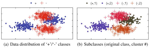
A toy example of finding subclasses and defining the respective sparse code vectors. (+, 1) : ${\mathbf{s}}_1^{(+)}=[\begin{array}{ccccc}+1& +1& 0& 0& 0\end{array}]$, (+, 2) : ${\mathbf{s}}_2^{(+)}=[\begin{array}{ccccc}+1& 0& +1& 0& 0\end{array}]$, (−, 1) : ${\mathbf{s}}_1^{(-)}=[\begin{array}{ccccc}-1& 0& 0& -1& 0\end{array}]$, and (−, 2) : ${\mathbf{s}}_2^{(-)}=[\begin{array}{ccccc}-1& 0& 0& 0& -1\end{array}]$.

Using the newly defined sparse codes, we assign a new label vector yⁱ to a training sample xⁱ as follows:

$${\mathbf{y}}^i={\mathbf{s}}_{{\gamma }_i}^{(y_i)}$$ (6)

where y_i ∈ {+, −} is the original label of the training sample xⁱ, and γ_i denotes the cluster to which the sample xⁱ was assigned by the K-means algorithm. In this way, we extend the original scalar labels of +1 or −1 into sparse code vectors in .

Thanks to our new sparse codes, it becomes natural to convert a single-task learning in Eq. (1) into a multi-task learning in Eq. (2) by replacing the original label vector y in Eq. (1) with a matrix $\mathbf{Y}={[{\mathbf{y}}^i]}_{i=1}^N\in {\{-1,0,1\}}^{N\times (1+K_{(+)}+K_{(-)})}$. Therefore, we have now (1 + K₍₊₎ + K₍₋₎) tasks. Note that the task of regressing the first column response vector y₁ corresponds to our binary classification problem between the original classes of ‘+’ and ‘−’. Meanwhile, the tasks of regressing the remaining column vectors ${\{{\mathbf{y}}_i\}}_{i=2}^{1+K_{(+)}+K_{(-)}}$ formulate new binary classification problems between one sub-class and all the other subclasses. It should be noted that unlike the single-task learning that finds a single mapping w between regressors X and the response y, the clustering-induced multi-task learning finds multiple mappings {w₁, · · ·, w_{(1+K(+)+K(−))}}, and thus allows us to efficiently use the underlying multipeak data distribution in feature selection.

3.3 Feature Selection and Classifier Learning

Because of the ℓ_2,1-norm regularizer in our objective function of Eq. (2), after finding the optimal solution, we have some zero row-vectors in W. In terms of the linear regression, the corresponding features are not informative in regressing the response values. In this regard, we finally select the features whose weight coefficient vector is non-zero, i.e., ||wⁱ||₂ > 0. With the selected features, we then train a linear Support Vector Machine (SVM) for making a diagnostic decision.

4 Experimental Results and Analysis

4.1 Experimental Setting

We considered three binary classification problems: AD/NC, MCI/NC, and MCI-C/MCI-NC. In the classification of MCI/NC, we labeled both MCI-C and MCI-NC as MCI. Due to the limited number of samples, we applied a 10-fold cross-validation technique in each binary classification problem. Specifically, we randomly partitioned the samples of each class into 10 subsets with approximately equal size without replacement. We then used 9 out of 10 subsets for training and the remaining one for testing. For performance comparison, we took the average of the 10 cross-validation results.

Regarding model selection, i.e., number of clusters K, sparsity control parameters of λ₁ in Eq. (1) and λ₂ in Eq. (2), and the soft margin parameter C in SVM [2], we further split the training samples into 5 subsets for nested cross-validation. To be more specific, we defined the spaces of the model parameters as follows: K ∈ {1, 2, 3, 4, 5}, C ∈ {2⁻¹⁰, . . . , 2⁵}, λ₁ ∈ {0.001, 0.005, 0.01, 0.05, 0.1, 0.15, 0.2, 0.3, 0.5}, and λ₂ ∈ {0.001, 0.005, 0.01, 0.05, 0.1, 0.15, 0.2, 0.3, 0.5}. The parameters that achieved the best classification accuracy in the inner cross-validation were finally used in testing.

To validate the effectiveness of the proposed Clustering-Induced Multi-Task Learning (CIMTL) method, we compared it with the Single-Task Learning (STL) method that used only the original class label as the target response vector. For each set of experiments, we used 93 MRI features and/or 93 PET features as regressors in the respective least square regression models. Regarding the neuroimaging fusion of MRI and PET [9], we constructed a long feature vector by concatenating features of the modalities. It should be noted that the only difference between the proposed CIMTL method and the competing STL method lies in the way of selecting features, i.e., single-task learning vs. multi-task learning. We used five quantitative metrics for comparison: ACCuracy (ACC), SENsitivity (SEN), SPECificity (SPEC), Balanced ACcuracy (BAC), and Area Under the receiver operating characteristic Curve (AUC).

4.2 Classification Results and Discussion

We summarized the performances of the competing methods with various modalities for AD and NC classification in Table 1. The proposed method showed the mean ACCs of 93.27% (MRI), 89.27% (PET), and 95.18% (MRI+PET). Compared to the STL method that showed the ACCs of 90.45% (MRI), 86.27% (PET), and 92.27% (MRI+PET), the proposed CIMTL method improved by 2.82% (MRI), 3% (PET), and 2.91% (MRI+PET). The proposed CIMTL method achieved higher AUC values than the STL method for all the cases. It is also remarkable that, except for the metric of SPEC with PET, 90.33% (STL) vs. 88.33% (CIMTL), the proposed CIMTL method consistently outperformed the competing STL method over all the metrics and modalities.

Table 1.

A summary of the performances for AD/NC classification

Method	Modality	ACC (%)	SEN (%)	SPEC (%)	BAC (%)	AUC (%)
STL	MRI	90.45±6.08	82.67	98.33	90.50	93.55
	PET	86.27±8.59	82.00	90.33	86.17	90.12
	MRI+PET	92.27±5.93	90.00	94.67	92.33	94.91
CIMTL	MRI	93.27±6.33	88.33	98.33	93.33	94.19
	PET	89.27±7.43	90.00	88.33	89.17	91.67
	MRI+PET	95.18±6.65	94.00	96.33	95.17	96.15

In the discrimination of MCI from NC, as reported in Table 2, the proposed CIMTL method showed the ACCs of 76.82% (MRI), 74.18% (PET), and 79.52% (MRI+PET). Meanwhile, the STL method showed the ACCs of 74.85% (MRI), 69.51% (PET), and 74.85% (MRI+PET). Again, the proposed CIMTL method outperformed the STL method by improving ACCs of 1.97% (MRI), 4.67% (PET), and 4.67% (MRI+PET), respectively. We believe that the high sensitivities and the low specificities for both competing methods resulted from the imbalanced data between MCI and NC. In the metrics of BAC and AUC that somehow reflect the imbalance of the test samples, the proposed method achieved the best BAC of 75.44% and the best AUC of 77.91% with MRI+PET.

Table 2.

A summary of the performances for MCI/NC classification

Method	Modality	ACC (%)	SEN (%)	SPEC (%)	BAC (%)	AUC (%)
STL	MRI	74.85±5.92	80.67	64.00	72.33	76.55
	PET	69.51±10.11	74.78	59.67	67.22	73.54
	MRI+PET	74.85±3.91	84.78	56.00	70.39	78.79
CIMTL	MRI	76.82±7.15	85.78	59.67	72.72	77.84
	PET	74.18±7.18	81.89	59.67	70.78	72.73
	MRI+PET	79.52±5.39	88.89	62.00	75.44	77.91

Lastly, we conducted experiments of MCI-C and MCI-NC classification, and compared the results in Table 3. The proposed CIMTL method achieved the best ACC of 72.02%, the best BAC of 70.33%, and the best AUC of 69.64% with MRI+PET. In line with the fact that the classification between MCI-C and MCI-NC is the most important for early diagnosis and treatment, it is remarkable that compared to the STL method, the propose method improved the ACCs by 4.62% (MRI), 5.15% (PET), and 7.4% (MRI+PET), respectively.

Table 3.

A summary of the performances for MCI-C/MCI-NC classification

Method	Modality	ACC (%)	SEN (%)	SPEC (%)	BAC (%)	AUC (%)
STL	MRI	56.98±20.61	51.00	60.67	55.83	58.85
	PET	61.58±17.79	55.00	66.00	60.50	60.63
	MRI+PET	64.62±14.04	62.50	66.00	64.25	63.87
CIMTL	MRI	61.60±13.12	44.00	75.67	59.83	60.76
	PET	66.73±11.32	39.00	88.00	63.50	65.57
	MRI+PET	72.02±13.80	58.00	82.67	70.33	69.64

For interpretation of the selected features, we built a histogram of the frequency of the selected ROIs of MRI and PET over CVs per binary classification. By setting the mean frequency as the threshold, features from the following ROIs were mostly selected: subcortical regions (e.g., amygdala, hippocampus, parahippocampal gyrus) and temporal lobules (e.g., superior/middle temporal gyrus, temporal pole).

Regarding the identified subclasses, we computed the statistics (mean±std) of the optimal number of clusters determined in our cross-validation: 2.5±1.7/2.5±1.2 (AD/NC), 3.1±1.1/2.9±1.2 (MCI/NC), 3.4±0.8/3.8±1.3 (MCI-C/MCI-NC). Based on these statistics, we can say that there exists heterogeneity in a group, and by reflecting such information in feature selection, we could improve the diagnostic accuracy.

5 Conclusion

In this paper, we proposed a novel method that formulates a clustering-induced multitask learning by taking into account the underlying multipeak data distribution of the original classes. In our experiments on the ADNI dataset, we proved the validity of the proposed method and showed its significantly better performance than the competing methods in the three binary classifications of AD/NC, MCI/NC, and MCI-C/MCI-NC.

References

- 1.de Brecht M, Yamagishi N. Combining sparseness and smoothness improves classification accuracy and interpretability. NeuroImage. 2012;60(2):1550–1561. doi: 10.1016/j.neuroimage.2011.12.085. [DOI] [PubMed] [Google Scholar]
- 2.Burges CJC. A tutorial on support vector machines for pattern recognition. Data Mining and Knowledge Discovery. 1998;2(2):121–167. [Google Scholar]
- 3.Fotenos A, Snyder A, Girton L, Morris J, Buckner R. Normative estimates of cross-sectional and longitudinal brain volume decline in aging and AD. Neurology. 2005:1032–1039. doi: 10.1212/01.WNL.0000154530.72969.11. [DOI] [PubMed] [Google Scholar]
- 4.Kabani N, MacDonald D, Holmes C, Evans A. A 3D atlas of the human brain. NeuroImage. 1998;7(4):S717. [Google Scholar]
- 5.Liao S, Gao Y, Shi Y, Yousuf A, Karademir I, Oto A, Shen D. Automatic prostate mr image segmentation with sparse label propagation and domain-specific manifold regularization. In: Gee JC, Joshi S, Pohl KM, Wells WM, Zöllei L, editors. IPMI 2013. LNCS. Vol. 7917. Springer; Heidelberg: 2013. pp. 511–523. [DOI] [PMC free article] [PubMed] [Google Scholar]
- 6.Mwangi B, Tian T, Soares J. A review of feature reduction techniques in neuroimaging. Neuroinformatics. 2013:1–16. doi: 10.1007/s12021-013-9204-3. [DOI] [PMC free article] [PubMed] [Google Scholar]
- 7.Noppeney U, Penny WD, Price CJ, Flandin G, Friston KJ. Identification of degenerate neuronal systems based on intersubject variability. NeuroImage. 2006;30(3):885–890. doi: 10.1016/j.neuroimage.2005.10.010. [DOI] [PubMed] [Google Scholar]
- 8.Sled JG, Zijdenbos AP, Evans AC. A nonparametric method for automatic correction of intensity nonuniformity in MRI data. IEEE Transactions on Medical Imaging. 1998;17(1):87–97. doi: 10.1109/42.668698. [DOI] [PubMed] [Google Scholar]
- 9.Suk HI, Lee SW, Shen D. Latent feature representation with stacked auto-encoder for AD/MCI diagnosis. Brain Structure and Function. 2013:1–19. doi: 10.1007/s00429-013-0687-3. [DOI] [PMC free article] [PubMed] [Google Scholar]
- 10.Suk HI, Wee CY, Shen D. Discriminative group sparse representation for mild cognitive impairment classification. In: Wu G, Zhang D, Shen D, Yan P, Suzuki K, Wang F, editors. MLMI 2013. LNCS. Vol. 8184. Springer; Heidelberg: 2013. pp. 131–138. [Google Scholar]
- 11.Varoquaux G, Gramfort A, Poline JB, Thirion B. Brain covariance selection: better individual functional connectivity models using population prior. In: Lafferty J, Williams CKI, Shawe-Taylor J, Zemel RS, Culotta A, editors. Advanced in Neural Information Processing Systems. 2010. pp. 2334–2342. [Google Scholar]
- 12.Zhu M, Martinez AM. Subclass discriminant analysis. IEEE Transactions on Pattern Analysis and Machine Intelligence. 2006;28(8):1274–1286. doi: 10.1109/TPAMI.2006.172. [DOI] [PubMed] [Google Scholar]