Coherent Flow Power Doppler (CFPD): Flow Detection using Spatial Coherence Beamforming

Abstract

Power Doppler imaging is a widely used method of flow detection for tissue perfusion monitoring, inflammatory hyperemia detection, deep vein thrombosis diagnosis, and other clinical applications. However, thermal noise and clutter limit its sensitivity and ability to detect slow flow. In addition, large ensembles are required to obtain sufficient sensitivity, which limits frame rate and yields flash artifacts during moderate tissue motion. We propose an alternative method of flow detection using the spatial coherence of backscattered ultrasound echoes. The method enhances slow flow detection and frame rate, while maintaining or improving the signal quality of conventional power Doppler techniques. The feasibility of this method is demonstrated with simulations, flow-phantom experiments, and an in-vivo human thyroid study. In comparison to conventional power Doppler imaging, the proposed method can produce Doppler images with 15-30 dB SNR improvement. Therefore, it is able to detect flow with velocities approximately 50% lower than conventional power Doppler, or improve the frame rate by a factor of 3 with comparable image quality. The results show promise for clinical applications of the method.

I. Introduction

Ultrasonic flow detection is a widely used technique to measure blood flow velocity [1], [2], monitor perfusion [3]–[5], detect hyperemia [6], diagnose thrombosis [7]–[11], and assess stenosis [12], [13]. Conventional techniques include color Doppler imaging and power Doppler imaging. These methods depend on either the phase change or the power of the backscattered echoes from blood. Color Doppler imaging estimates the axial blood velocity from temporal changes in the echo phase. Because the measurement of blood velocity may be sensitive to noise [14], color Doppler imaging has sub-optimal performance with small vessel and slow flow. Power Doppler imaging measures the power of the temporal differences in backscattered echoes, and can provide higher sensitivity with small vessel and slow flow detection at the expense of direction information [15]. However, it requires a large ensemble length, limiting the frame rate to a few frames per second.

The potential noise sources that degrade power Doppler imaging include clutter and thermal noise. Clutter originates from sound reverberations in tissue layers, scattering from off-axis structures, ultrasound beam distortion, and returning echoes from previously transmitted pulses [16]. Clutter is stationary with respect to time and obscures blood vessels and other clinical targets. In cardiac imaging, stationary echoes may be 40 to 100 dB stronger than the signal from blood [17]. In conventional Doppler imaging, high-pass wall filters are commonly used to remove stationary echoes. However, the small number of samples (8 to 16) available to the wall filter reduces the ability of the wall filter to effectively reject unwanted signals [17], and stationary echoes may pass through the wall filter depending on their magnitude of temporal frequency content. Thermal noise (i.e. electronic noise) is a temporally and spatially white noise process and appears as a rapidly moving target in the ensemble. Therefore, it cannot be removed with wall filters typically used in Doppler imaging. If any of these types of noise has comparable power as the blood signal after wall filtering, they will degrade the quality of the power estimate. Although considerable efforts have been made to improve the image quality and frame rate of Doppler imaging techniques using novel sequence designs such as synthetic aperture [18] and μDoppler sequences [14], the aforementioned noise sources still impose significant limitations on the performance of Doppler imaging.

Short-lag spatial coherence (SLSC) imaging was recently introduced as an imaging method that forms ultrasound images using the spatial coherence information of backscattered echoes [19]. It makes use of a classical theorem of statistical optics, the van Cittert-Zernike (VCZ) theorem, which describes the equal-time degree of coherence in a field generated by a spatially incoherent quasi-monochromatic source [20]. The expression of the VCZ theorem bears close resemblance with the Huygens-Fresnel principle and the Fraunhofer diffraction at an aperture. Mallart and Fink [21] and Liu and Waag [22] generalized this theorem to pulse echo ultrasound imaging, and showed that the spatial covariance of the backscattered pressure field at the transmit focus is proportional to the autocorrelation of the transmitting aperture function. A similar result was also derived using a k-space representation by Walker and Trahey [23].

The SLSC method computes the normalized covariance of the signals received on every pair of elements of the transducer, denoted by s_i(n) for element i and s_i+m(n) for element i + m of the transducer, in which n is the fast-time index. The normalized covariance of the signal is defined as

$$\widehat{R}(m)=\frac{1}{N-m}\sum _{i=1}^{N-m}\frac{{\sum }_{n=n_1}^{n_2}{s}_i(n)s_{i+m}(n)}{\sqrt{{\sum }_{n=n_1}^{n_2}{s}_i^2(n){\sum }_{n=n_1}^{n_2}{s}_{i+m}^2(n)}},$$ (1)

in which m, defined as lag, is the spacing of elements between element i and element i + m. R̂(m) represents the normalized covariance of the signals received on the pairs of elements with lag m, and N is the number of transducer elements in the active aperture. n₂ – n₁ is the kernel size for cross-correlation calculation.

The spatial correlation in Equation (1) can then be used to produce the SLSC metric. The metric is computed by summing the spatial correlation values produced with Equation (1) corresponding to the smallest M lags

$$V_{\mathit{\text{slsc}}}=\sum _{m=1}^M\widehat{R}(m).$$ (2)

An SLSC image is produced by computing the V_slsc value for each pixel. A parameter Q is introduced to represent M as a percentage of the receive aperture size:

$$\mathrm{Q}=\frac{M}{N}\times 100\%$$ (3)

It has been shown that the spatial coherence backscattered from tissue is considerably higher than adjacent anechoic or hypoechoic regions [19]. Using this difference in spatial coherence, the technique has been shown to produce images resembling those produced by conventional delay-and-sum beamforming. In addition, because thermal noise and clutter are often spatially incoherent (i.e. R̂(m) ≈ 0, for m > 0), the SLSC imaging technique is less susceptible to such noise sources and artifacts than conventional delay-and-sum beamforming. It can produce images with higher speckle SNR and higher contrast-to-noise-ratio (CNR) [19] [24]. The method has been extended to harmonic spatial coherence imaging [25] and synthetic aperture SLSC imaging [26] to further improve image quality and mitigate depth of field limitations of the method.

Herein, we describe a recent development in a coherent flow imaging technique, termed Coherent Flow Power Doppler (CFPD) imaging, that is based on the spatial coherence of the blood signal. This technique utilizes a similar pulse sequence as conventional power Doppler (PD) imaging, but obtains and images spatial coherence information of the backscattered signal [19]. The performance of this technique is evaluated under various flow velocities and channel SNR using simulations, phantom experiments, and in-vivo studies. The image quality and limit of detection are benchmarked with those of a conventional PD technique.

The article is organized as follows: Section II presents the principles of CFPD imaging; Section III describes the methods utilized in the simulations, phantom studies, and in-vivo studies; Sections IV analyzes the results from these studies, evaluates the performance of CFPD, and compares its performance with PD; and Section V and VI present further discussion and conclusions.

II. Principles of Coherent Flow Imaging

A. Power Doppler imaging

Conventional power Doppler (PD) imaging requires an ensemble of RF traces to estimate the presence of flow. An ensemble of 8-16 RF lines is acquired at each azimuthal position in a Doppler image. The A-scans are acquired at a fixed pulse-repetition frequency (f_prf) focused at the same location and beamformed using delay-and-sum beamforming. The focus is shifted to the next location, and the next A-scan ensemble is acquired in the same way. The A-scans from each location can also be interleaved to improve frame rate and control the pulse repetition rate. Because the ensemble of A-scans contain stationary echoes from tissue that may overpower the blood signal, a high-pass wall filter is applied to the A-scan ensemble to attenuate any stationary and slowly changing signal in order to obtain flow information. A PD image is produced by applying a power estimator to the filtered signal. A commonly used estimator, proposed by Loupas et al. [27] and based on a two-dimensional (2D) autocorrelator, for blood flow estimation is:

$$\text{PD}=\sum _{k=1}^K\sum _{p=1}^P{|r(k,p)|}^2,$$ (4)

in which r(k, p) is the high-pass filtered complex signal at depth sample k and ensemble sample p. K is the number of samples summed in the axial dimension; and P is the ensemble length.

Equation (4) shows that the output signal of PD is dependent on the energy of the signal. This technique does not measure the velocity of flow. For flow at a fixed velocity, the strength of PD signal is associated with the number of scatterers in the voxel to a first approximation [28]. It has higher sensitivity for slow flow and small vessel detection than color Doppler imaging [15].

One problem with PD is that the high-pass filter requires a large number of samples (i.e. a large ensemble length) to achieve steady-state performance with high attenuation in the stopband. This is not ideal for clinical applications because a very large ensemble length reduces the frame rate and is susceptible to flash or motion artifact. Therefore, the filters used in Doppler imaging operate in their transient state with inferior performance, due to a wider transition band and lower attenuation in the stop band (see Fig. 1).

Fig 1.

A comparison of transient state and steady state frequency responses of a high-pass 2-tap Butterworth filter with projection initialization. H(f) denotes the frequency response of the filter. The frequency axis is normalized to the Nyquist frequency. The cutoff frequency is 5% of the Nyquist frequency. In the transient state, the filter has lower attenuation in the stopband and a wider transition band than the steady state.

Reverberation clutter can appear similar to slowly moving blood. Therefore, the attenuation applied by the wall filters on reverberation clutter and slowly moving tissue may not be strong enough, and such noise may pass through the wall filter and degrade the power Doppler image. In addition, if the flow velocity is too low, the flow signal may fall into the transition band of the filter and may be attenuated. If the power of the thermal noise is higher than the backscattered signal energy from blood, the flow signal will not be differentiable from the background.

B. Coherent flow imaging

Coherent flow imaging utilizes SLSC beamforming to obtain coherence information of flow, and then utilizes a power estimator to produce an image that resembles the conventional PD images. Fig. 2 presents an outline of CFPD for coherent flow imaging, as well as a comparison of CFPD with PD. In coherent flow imaging, the pulse sequence is identical to conventional PD imaging, however, the method requires individual channel RF data, rather than the beamformed data in the case of PD imaging. These RF channel data from all acquisitions are delayed according to path length differences and filtered across the ensemble on a per-channel basis to remove stationary signals and slowly moving tissue signals and isolate the blood signal.

Fig 2.

Signal processing path of CFPD and PD. For both CFPD and PD, RF channel data are first (a) acquired at one focused lateral location at a fixed f_prf, and then (b) time delayed. For CFPD, the delayed data are (c) high-pass filtered across the ensemble length, and then (d) processed with the SLSC method. (e) A power estimator is used to produce one A-scan, and the whole process is repeated for all lateral positions to produce one Doppler image frame. For the PD method, the delayed data are (f) summed across the receive aperture, and (f) high-pass filtered across the ensemble length. (h) A power estimator is used to produce one A-scan, and the whole process is repeated for all lateral positions to produce a Doppler image frame.

The filtered RF channel data for each scan in the ensemble are processed using the SLSC method described in Section I to obtain the spatial coherence of backscattered signal from blood. Based on the preliminary results presented in Section III.A, a lag of M = 10, corresponding to Q = 7.8% is chosen to be used in all data processing in this work. In order to produce Doppler images, a modified Loupas estimator is then applied to the data to produce Doppler information. Specifically, the square of the SLSC values is added across the ensemble dimension:

$$\text{CFPD}=\sum _{p=1}^P{V}_{\mathit{\text{slsc}}}^2(p),$$ (5)

where V_slsc(p) is the SLSC signal calculated with Equation (2) for the pth acquisition, and P is the ensemble length used in the estimator. Note that for B-mode SLSC, V_slsc(p) is calculated from time-delayed RF channel data, but for CPFD, V_slsc(p) is calculated from time-delayed and high-pass filtered RF channel data.

III. Methods

A. Simulations

Simulations were performed with Field II [29], [30] to observe the performance of CFPD for various flow velocities under different noise conditions. In the simulations, a 2 mm vessel was embedded in homogeneous tissue. The setup and an example Doppler image are shown in Fig. 3. Blood signal within the vessel was simulated by scatterers with scattering amplitude 60 dB lower than the surrounding tissue scatterers. The peak velocity of the scatterers within the vessel was varied from 1 to 30 mm/s with a parabolic velocity profile in order to study the change in performance of the method with respect to different flow velocities. This range covers the blood flow velocity of human capillaries (e.g. the velocity of capillary blood flow in postocclusive reactive hyperemia is 0.9 mm/s [31], and veinous and arterial blood flow velocity in human retina is 19 - 22 mm/s) [32]). The scatterer density for both the blood and the surrounding tissue was 15 scatterers per resolution voxel. The simulations were conducted with a 128-element linear transducer array with a center frequency of 7.5 MHz and a pitch of 0.1953 mm. The transmit pulses had a fractional bandwidth of 35% and were focused at 3 cm.

Fig 3.

A map of the flow velocities in the simulated phantoms. The peak velocity shown in this image is 30 mm/s. The colored region in the center indicates the location and size of the vessel. In the vessel, the blood flow velocity has a parabolic profile. The dashed boxes indicated the locations of background signal in SNR measurement. The scale bars on the bottom right of the image indicate 1 mm, and the color scale indicates flow velocities with units of mm/s.

Simulated channel data were acquired at a sampling rate of 40 MHz for a lateral field-of-view of 12 mm with 0.1 mm beam spacing. For each location, an ensemble of 15 A-scans was acquired at an f_prf of 1 kHz, and the channel signals were appropriately delayed. Thermal noise was simulated by adding white noise to the delayed channel data. The noise amplitude was added in the range of -20 to 0 dB relative to the blood signal (i.e. -60 to -80 dB relative to the tissue signal). In order to observe the effect of ensemble length on image quality, the data were truncated in the ensemble dimension into different sets with ensemble lengths ranging from 3 to 15 with the same f_prf. Each of the truncated data sets were processed separately. The data in each set were filtered with a 2-tap projection-initializated Butterworth filter with a cutoff frequency of 5 Hz to remove stationary clutter. The filtered data were then processed with the method described in Section II.B to produce CFPD images. In order to reduce image size, only a lateral FOV of 5 mm about the center of the vessel is shown. The remaining region is used in the SNR measurement as part of the background and does not have any features of interest. As a comparison, the same data were also processed with conventional PD imaging method described in Section II.A.

B. Phantom and in-vivo studies

Phantom and in-vivo studies were conducted with a Verasonics Vantage system (Verasonics, Inc., Redmond, WA) and an ATL L12-5 linear transducer. The transducer transmitted 6 half-wave (3 full cycles) pulses. The center frequency of the pulses is 5 MHz. 128 transducer elements were used to generate the transmit wave that focused at 5 cm, corresponding to an F/2 configuration. For each acquisition, the RF channel signals for 50 locations (for a total width of 9.8 mm) were obtained for an ensemble size of 15 and an f_prf of 1 kHz. In addition, one B-mode scan of 129 lateral lines was also acquired, centered about the same location. All data were sampled at 19.2 MHz.

In the phantom experiments, a continuous-flow pump and cardiac Doppler flow phantom (Model 523, ATS Laboratories, Inc., CT) system was used to circulate a 3% (mass/mass) cornstarch-water mixture through a 6 mm vessel inside the flow phantom with speeds ranging from 11.5 mm/s to 274 mm/s. The phantom has a mean acoustic velocity of 1452 m/s, and the fluid has a density of 1030 kg/m⁻³ and speed of sound of approximately 1531 m/s. The velocity of flow was calibrated by measuring the weight of fluid pumped over a fixed period of time.

In the in-vivo study, thyroid scans from a 26-year-old healthy male volunteer were acquired in the same way after obtaining informed consent. The vessel was identified using the prepackaged, real-time, power Doppler imaging method on the Verasonics scanner, and the channel data were saved to be processed and analyzed off-line.

All data from the phantom and in-vivo studies were processed with the method described in Section II.B to produce CFPD images. The data were also processed with the method described in Section II.A to produce conventional PD images. The filter cut-off frequency was chosen to be 150 Hz for the phantom studies and 200 Hz for the in-vivo studies. In order to provide better visualization of the data, the dynamic ranges of the Doppler images were compressed with a base-10 logarithmic function.

C. CFPD with novel sequence designs

CFPD is not dependent on specific pulse sequences. As demonstrated previously with SLSC, this beamforming method can be applied in conjunction with pulse-inversion harmonic [25] and synthetic aperture imaging [26]. CFPD has the potential to utilize recent advancements in novel sequence design in Doppler imaging, such as plane-wave transmit with coherent angular compounding (termed μDoppler) [14] and synthetic aperture flow imaging [18]. As proof-of-concept, CFPD flow detection is experimentally demonstrated in-vivo with plane-wave transmit coherent angular compounding.

The experiment was carried out with the same setup as in the phantom and in-vivo studies. Specifically, an ATL L12-5 transducer is used with a Verasonics Vantage system. The transmit center frequency was 5 MHz, and receive data were sampled at 19.2 MHz.

For transmit, the entire aperture of 128 elements were used to sequentially transmit 15 plane waves evenly spanning an azimuthal angular range of -18 to 18 degree. The transmit interval between acquisitions at adjacent angles is 133 μs, corresponding to an effective f_PRF of 500 Hz. An ensemble size of 15, each from the coherent compounding of 15 angles, was acquired. The details of beamforming with plane-wave transmit and coherent angular compounding can be found in Mace et al. [14]. However, in this application, the channel signals are synthesized for the CFPD process rather than the delay-and summed RF signals.

The plane-wave sequence was used to acquire liver scans on a 57-year-old healthy male with high body mass index (> 25). Time delay and coherent angular compounding were performed on the data according to Mace et al. [14] to obtain synthesized channel signal. CFPD was applied to the data to produce flow information. As a comparison, PD images are also created from the synthesized channel signal. All images are displayed with base-10 logarithmic compression and a dynamic range of 30 dB.

D. Image quality metrics

The quality of the simulated and experimental Doppler images are evaluated in two aspects: the strength of the signal, and the defects in the signal. The strength of the signal directly affects the detection of the presence of flow, and the defects in the shape and smoothness of the intensity profile affect the quality of estimates on the size and number of vessels. Signal-to-noise ratio (SNR) and contrast-to-noise ratio (CNR) were used to measure the quality of images in these two aspects, respectively.

The SNR measures the strength, or power, of the signal relative to the power of the noise. It is defined as the ratio between the root-mean-square (RMS) of signal from the vessel and the RMS of the background region:

$$\text{SNR}=20\cdot {log}_{10}\left(\frac{\sqrt{\frac{1}{N}\cdot \sum _{i=1}^N{\mathrm{I}}_{\mathit{\text{sig}}}^2(i)}}{\sqrt{\frac{1}{M}\cdot \sum _{i=1}^M{\mathrm{I}}_{\mathit{\text{bkgd}}}^2(i)}}\right),$$ (6)

where I_sig(i) represents the value at the i-th pixel in the vessel region in the Doppler images; N is the total number of pixels used for SNR measurement in the vessel region; I_bkgd(i) is the pixel value at the i-th pixel in the background; and M is the total number of pixels used in the background region. The vessel region was determined with known vessel diameters and center locations in the simulations and experiments. The background region used for SNR measurement was chosen such that it was at the same depth as the vessel region, as shown in Fig.3.

The definition of CNR is adopted from Lediju et al. [19] as

$$\text{CNR}=20\cdot {log}_{10}\left(\frac{|S_{\mathit{\text{sig}}}-S_{\mathit{\text{bkgd}}}|}{\sqrt{{\sigma }_{\mathit{\text{sig}}}^2+{\sigma }_{\mathit{\text{bkgd}}}^2}}\right),$$ (7)

where S_sig and S_bkgd are the mean of the pixel values in the signal region and the background region, respectively; and σ_sig and σ_bkgd are the standard deviation of the pixel values in these regions. CNR quantifies detection of a signal with noise. It takes into account both the mean values and the fluctuations inside both signal region and background region.

IV. Results

A. Normalized covariance measurement of tissue and fluid

Fig. 4 presents measured normalized covariance R̂(m) curves as a function of lag for stationary tissue, fluid, and thermal noise. The stationary tissue data was acquired on the liver of a 57-year-old healthy male subject, after informed consent was obtained. The fluid data was from the phantom study with a flow velocity of 11.5 mm/s and an ensemble length of 15. As shown in the figure, the normalized covariance of both tissue and fluid share similar characteristics in the short-lag region (Q < 30%). In this region, they have higher values than the normalized covariance of thermal noise. The normalized covariance of tissue and fluid are higher than that of reverberation clutter as shown previously [33]. Because the backscattered signal from blood has the same coherence properties as tissue, CFPD processing on blood signal will result in high values in the final image. Because thermal noise and reverberation clutters have low coherence, they will be suppressed in the CFPD computation.

Fig 4.

An example of normalized covariance, R̂(m), from an in-vivo stationary tissue sample, moving fluid, and thermal noise. The abscissa represents the lag as a percentage of the aperture size; the ordinate represents normalized covariance. The stationary tissue and moving fluid exhibit similar spatial coherence profiles. In the short-lag region (Q < 30%), they have higher values than thermal noise.

B. Simulations

Fig. 5 presents a comparison of simulated CFPD and PD images for four different flow speeds (5 mm/s, 7 mm/s, 15 mm/s, and 30 mm/s) with -10 dB noise added to the channel data. The images are shown on a base-10 logarithmic scale with a dynamic range of 30 dB. The CFPD images are on the left of each image set, and the PD images are on the right. A cross-section of a 2 mm vessel can be observed in the figures. The CFPD images have lower background noise than the PD images generated from the same simulation data and the flow region in the CFPD images displays a smoother and fuller profile. Both methods show improved signal quality for higher flow speeds. The displayed image quality can be improved by individually tuning the dynamic range of each image. Therefore, quantitative analysis was performed on the CFPD and PD images for a more objective comparison.

Fig 5.

Simulated CFPD (left) and PD (right) images for different flow speeds. Speeds: (a) 5 mm/s; (b) 7 mm/s; (c) 15 mm/s; (d) 30 mm/s. The diameter of the vessels is 2 mm. An ensemble length of 15 was used to produce the images, and -10 dB noise is added. The scale bar in the right corner indicates 1 mm, and the colorbars have units of dB. The dynamic range is 30 dB for all images. The CFPD images show lower background noise than the PD images.

Fig. 6 shows the quantitative SNR measurement for both the simulated CFPD and PD images as a function of flow speed. Three different levels of noise (0 dB, -10 dB, and -20 dB relative to blood signal) were added to the channel data, and all 15 scans in the ensemble were used. The SNR of the CFPD images is significantly higher than that of the PD images.

Fig 6.

The SNR of simulated images acquired in simulations with different flow speeds. Different levels of white noise, relative to the blood signal, were added to the channel data: (a) 0 dB; (b) -10 dB; (c) -20 dB. The dashed line indicates the detection threshold. CFPD has a 15-30 dB SNR advantage over PD with speeds ranging from 12 to 25 mm/s. The limit of detection in speed is lower by approximately 50% with CFPD.

The SNR was used to determine the limit of detection (LOD) of the flow velocity (v). Specifically, the signal at velocity v is considered detectable if

$$\text{SNR}(v)>3\cdot {\sigma }_{\text{SNR}},$$ (8)

where SNR(v) represents the mean of the SNR measurement at velocity v, and σ_SNR is the standard deviation of all SNR measurements.

This criterion, with the factor 3 on the right-hand side, was chosen according to a well-established standard in LOD determination [14], [34]. According to the criterion, a threshold of 10 dB in SNR was utilized, based on the measurement of σ_SNR, to determine the LOD in flow velocity with both methods. The LOD for CFPD was measured to be 52.2%, 52.5%, and 62.1% lower than conventional PD for 0 dB, -10 dB, and -20 dB noise, respectively. This result indicates that CFPD may allow detection of slower flow than conventional PD.

Figs. 7 and 8 display the simulated images and the SNR measurements, respectively, with different ensemble lengths for a flow rate of 20 mm/s. As shown in Fig. 8, CFPD produces images with 15-30 dB higher SNR than conventional PD. Due to this improvement, CFPD may require only 7 acquisitions to produce images comparable to, or better than, conventional PD images produced from 15 acquisitions. If 10 dB SNR is utilized as the threshold of detection, CFPD requires only 3 acquisitions to produce useful Doppler images in a low noise environment (e.g. -20 dB white noise).

Fig 7.

Simulated CFPD (left) and PD (right) images with different ensemble lengths (a)-(f) for flow of 20 mm/s with 0 dB noise (high noise case), relative to the blood signal. The vessel diameter is 2 mm. The scale bar on the right corner indicates 1 mm, and the colorbar has units of dB. The dynamic range is 30 dB for all images. The figure shows better SNR and lower background noise in the CFPD images.

Fig 8.

SNR of simulated blood flow with different ensemble lengths. The flow speed is 20 mm/s. Three levels of noise were added to the channel data: (a) 0 dB; (b) -10 dB; (c) -20 dB. The dashed line indicates the 10 dB detection threshold. In general, CFPD produces images with 15-25 dB higher SNR than conventional PD, enabling flow detection with fewer acquisitions.

Fig. 9 displays the performance of the CFPD and PD methods as a function of noise. For PD, the delay-and-sum beamformer with 128 transducer elements improves the SNR by approximately 20 dB. CFPD, however, provides an additional 15-30 dB improvement in SNR in this range. For example, with -20 dB channel amplitude noise, the image SNR with PD is approximately 56 dB, and the image SNR produced with CFPD is 73 dB.

Fig 9.

SNR measurement of simulated images as a function of channel SNR. The flow velocity is 20 mm/s for all cases. An ensemble length of 15 was used to produce the Doppler images. In general, CFPD produces images with 15-30 dB higher SNR than the conventional PD method, enabling flow detection in more noisy environments.

C. Phantom studies

Fig. 10 presents the Doppler images with flow velocities ranging from 11.5 to 274 mm/s. Both the CFPD and PD images were produced with all 15 acquisitions in the ensemble. The dynamic range of the Doppler images is 30 dB. The Doppler images are fused with the B-mode images of the same region. The Doppler images are only shown in the center ±5 mm regions of the images, indicated with the dashed white lines in Fig. 10 (a). As shown in the figure, CFPD produces Doppler images with high quality for all velocities utilized. The size of the detected flow is consistent with the vessel diameter. The CFPD image also demonstrates a smooth intensity profile. PD produces images with discontinuity and inhomogeneity (Fig. 10 (a), and (b)), and spurious signals at the lower part of the images from thermal noise (Fig. 10 (a)).

Fig 10.

CFPD (left) and PD (right) images from the phantom experiments with different flow velocities, produced with all 15 acquisitions in each ensemble. The scale bar on the right corner indicates 4 mm, and the colorbar has units of dB. Doppler imaging is shown in the center ±5 mm region of the lateral FOV. The dynamic range is 30 dB for all images. The figure shows better SNR and lower background noise in images produced using CFPD. At low velocity (a), the PD image displays higher noise in the lower part of the scan, due to loss of SNR with depth.

Fig. 11 shows the Doppler profile at the center of the lateral FOV from the phantom study with 11.5 mm/s flow and an ensemble length of 15. For the PD image, an increase in the background noise can be observed over depth. In comparison, the CFPD result has a relatively constant background noise level across the axial dimension, indicating that CFPD is insensitive to thermal noise.

Fig 11.

Center axial line of the CFPD and PD images shown in Fig. 10 (a). PD shows an increase in noise from -50 dB to approximately -25 dB in the depth dimension. CFPD has a constant low noise level of approximately -65 dB across all depths, indicating that CFPD is insensitive to thermal noise.

Fig. 12 shows the SNR and CNR measurement from the flow-phantom studies with different flow speeds, processed with an ensemble length of 15. CFPD shows better SNR and CNR than PD for the speed range 11.5 - 274 mm/s. The CNR measurement from CFPD shows consistently higher values than PD.

Fig 12.

SNR and CNR measurement from flow phantom experiments. All 15 acquisitions in each ensemble were used. For the speed range of 11.5-274 mm/s, CFPD shows higher SNR and higher CNR.

Fig. 13 presents CFPD and PD images in the phantom experiments with different ensemble lengths. The flow velocity used for the image is 11.5 mm/s. As shown in Fig. 13 (a) and (b), with a small ensemble length (3 and 5 respectively), PD produces flow images with strong inhomogeneity and high variance. CFPD is also affected by low ensemble lengths, but the Doppler image it produces has a low variance. With higher ensemble lengths, PD produces images with less thermal noise, but noise is still visible in the lower part of the image. The CFPD images lack visible artifacts from thermal noise.

Fig 13.

CFPD (left) and PD (right) images of 11.5 mm/s flow in the phantom experiments with different ensemble lengths. The scale bar on the right corner indicates 4 mm, and the colorbar has units of dB. The dynamic range is 30 dB for all images. The figure CFPD images show better SNR and lower background noise than PD. The PD image suffer from higher background noise at deeper depth.

Fig. 14 shows the SNR and CNR measurement for both CFPD and PD images with different ensemble lengths at the lowest velocity used in the phantom experiments (11.5 mm/s). CFPD provides a consistent improvement of 15-30 dB in SNR. The CNR of the CFPD images is also higher, indicating that CFPD produces a smoother flow map within the vessel. For the phantom experiments, CFPD required only 5 acquisitions in an ensemble to produce a Doppler image with higher SNR and CNR than the image produced by PD with 15 acquisitions.

Fig 14.

SNR and CNR measurement from flow phantom experiments with different ensemble lengths. The flow velocity for all cases is 11.5 mm/s. CFPD shows higher SNR and higher CNR for all cases.

D. In-vivo studies

A Doppler scan of the thyroid of a healthy human subject is shown in Fig. 15. The Doppler data are displayed on a dB scale with a dynamic range of 30 dB. The Doppler image is fused with the B-mode image acquired at the same time. The lateral range of the Doppler scan is restricted to the center ±5 mm center of the B-mode image. Images from both methods show two vessels in the field of view. However, PD displays high thermal noise, especially in the lower part of the image.

Fig 15.

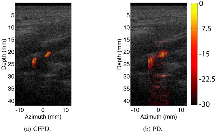
In-vivo thyroid Doppler images. The colorbar has units of dB. The dynamic range is 30 dB for all images. CFPD and PD both show two vessels in the field of view. The PD image shows higher thermal noise, especially in the lower part of the image.

E. CFPD with novel sequence designs

Fig. 16 shows in-vivo liver Doppler images created with plane-wave transmit coherent angular compounding sequence. The images from two scan locations of the liver are shown. The abdominal layers are visible in all images. In the Doppler images of Location 1, CFPD shows a homogeneous image of a vessel. The PD image shows a broken and granular image of a vessel. At location 2, PD fails to show vessels at deep tissue, because the signal is overwhelmed by thermal noise. In contrast, CFPD shows the locations of several liver vessels.

Fig 16.

In-vivo liver Doppler images produced with plane-wave transmit coherent angular compounding sequence. Two locations were scanned and processed with both CFPD and PD methods. The results were presented with the same dynamic range (30 dB). In the Doppler images of Location 1, CFPD shows a homogeneous image of a vessel. The PD image shows a broken and granular image of a vessel. At location 2, PD fails to show vessels at deep tissue, while CFPD shows the locations of the vessels.

Shows in-vivo liver Doppler images created with a plane-wave transmit coherent angular compounding sequence.

V. Discussion

We have introduced a coherent flow imaging method using the spatial coherence of backscattered signal from blood, termed CFPD. Compared with conventional power Doppler imaging, CFPD showed a gain of 15-30 dB in SNR under equivalent imaging conditions. This gain is ascribed to the fact that CFPD is less susceptible to spatially incoherent noise, such as thermal noise and reverberation echoes, which may overwhelm flow signals for conventional PD imaging. As a result, the CFPD images show consistently lower background noise, especially in deep-lying tissues, where thermal noise is more prevalent in conventional PD images. The improvement on SNR results in an increase in display dynamic range for CFPD. Although the contrast of PD image can be improved by limiting the display dynamic range, it is often at the expense of features in the image. Moreover, as shown in the results (see Fig. 5 and 7), higher thermal noise in the channel data causes more severe washout in PD images, but such noise does not have high impact in the background of the CFPD images. As shown in the experimental results (Fig. 11), CFPD is insensitive to the increase in thermal noise with depth, as observed in PD. Clinical scanners may avoid such spurious signals in deeper part of the PD images by limiting the display window size, although not always eliminating the problem particularly when the vessels themselves are at larger depths.

With increased SNR, CFPD results in improved performance in multiple aspects over PD. First, slow flow that is below the LOD of PD can be detected using CFPD, where it was shown that velocities approximately 50% lower than the LOD of PD could be detected, depending on SNR. Such an improvement may enable flow detection with velocities of 3-10 mm/s for the imaging frequencies and probes utilized in these experiments. Recent development in Doppler imaging enables detection of flow at such velocities either with high-frequency (15 MHz) acoustic pulses [35], and thus has low penetration depth and low SNR due to the plane-wave transmit technique used, or with contrast agents [36]. However, the results presented in this paper demonstrate that improved detection can be obtained without a loss in penetration depth or by utilizing additional contrast agents. This method can also utilize existing beamforming methods, such as higher harmonic imaging or synthetic aperture imaging, to obtain further enhancements.

The source of CFPD performance improvement demonstrated here is the suppression of thermal noise, which is spatially and temporally incoherent. We anticipate that stationary clutter, which has lower spatial coherence than flow signal, will also be suppressed with CFPD, but this was not analyzed in detail here. Slow flow signal is highly coherent temporally. As flow speed increases, the temporal coherence of the flow signal decreases, and flow signal appears more similar to thermal noise in its temporal aspect. The sum of N temporally coherent signals (e.g. slow flow signal) increases by a factor of N, whereas the sum of N temporally incoherent signals (e.g. thermal noise or fast flow signal) increases by a factor of √N. Therefore, if the impact of ensemble lengths on filter performance is ignored, the SNR of PD images increases proportional to √N for slow flow cases, and approaches a constant for fast flow cases. The SNR of CFPD is similarly affected. However, due to the suppression of noise, the SNR of CFPD is higher than PD and therefore reaches a constant SNR value much quicker than PD when flow speed is increased (see Fig. 6). As shown in Section IV for physiological cases, the SNR of CFPD method is still higher than the conventional PD method because of the suppression of noise.

It is important to keep in mind the physical meaning of the output of the SLSC beamformer applied to the CFPD technique. CFPD is based on the spatial coherence of backscattered waves, rather than the amplitude of the waves. In Equation (1), the coherence values are normalized by their variance in time, removing any impact of scattered wave amplitude (or power) on coherence. The coherence values are constructed almost exclusively with the phase difference between the signals. Therefore, the amplitude of the scattered wave has little impact on the output of the SLSC beamformer. Demonstrations of SLSC beamforming [19], [24]–[26] have shown comparable output to DAS B-mode imaging, and therefore the power estimator for CFPD in Equation (5) is a natural extension of a power estimator for PD.

It is worth mentioning that, in the case of low channel noise and high flow signal, lateral “side lobes” can be observed in the CFPD images. These side lobes appear because of re-correlation of the strong off-axis blood signal. The lateral cross-sections of simulated flow signals at the center of vessels produced with 30 mm/s flow, an ensemble length of 15, and two different channel noise levels (0 dB and -20 dB) are shown in Fig.17. “Side lobes” are visible for the -20 dB noise case near ±3 mm lateral locations. These side lobes reduce SNR of the CFPD images. However, the magnitude of the side lobes is 60 dB below the flow signal. These side lobes are lower than the typical display range of Doppler images. In addition, the “side lobes” appear only when the channel noise is relatively low (-20 dB relative to blood signal) and the flow velocity is high, because with higher noise, the off-axis signal is overwhelmed by the thermal noise. At these high velocities and low noise levels, however, there is less need for CFPD, because the vessels are often detectable by normal methods.

Fig 17.

Lateral side lobes in CFPD images, produced with high flow velocity (30 mm/s), an ensemble length of 15, and two different channel noise levels (0 dB and -20 dB). The curves represent the lateral cross-sections of at the center of vessels in the simulation results. For the low noise case (-20 dB), side lobes can be observed near ±3 mm lateral locations. The magnitude of the side lobes are approximately 60 dB below flow signal level. With higher noise (0 dB), the side lobes are not present.

A second improvement that may have greater value for clinical applications is the higher frame rate afforded by CFPD. Due to the improvement in SNR, CFPD can use an ensemble length of 3 to 7 to produce the same quality of Doppler image as PD with an ensemble length of 15. The significance of this result is that, assuming negligible computational time, CFPD can perform Doppler imaging at a frame rate 3 times higher PD with less degrading effects from noise.

CFPD utilizes an identical acquisition sequence as PD, and produces Doppler images with comparable scale. Therefore, CFPD is portable to clinical scanners. In addition, CFPD is not dependent on a specific acquisition sequence and thus is not limited to the sequences demonstrated in this work. As with SLSC imaging, which has been shown to perform well in harmonic imaging [25] and synthetic aperture imaging [26], CFPD can utilize the RF channel data from other types of power Doppler imaging methods to produce CFPD images. For example, it can take advantage of the latest developments in Doppler sequence design [14], [18] to further increase frame rate. It is demonstrated that CFPD can be utilized in conjunction with the plane-wave transmit coherent angular compounding technique. Plane-wave transmit coherent angular compounding has previously been demonstrated with ultrasfast Doppler imaging [14], [37]. The combination of this synthetic transmit aperture technique and Doppler imaging suffers from poor SNR because of the low number of transmits contributing to the synthetic transmit. Fig. 16 demonstrates improved flow detection deep in the human body (6.7 cm) with this synthetic aperture technique combined with CFPD, and shows that CFPD is a method that can be utilized in conjunction with and improve upon other novel imaging sequences. The flexibility of CFPD may allow wider use of in both the clinical and research settings.

VI. Conclusion

We have presented a method of flow detection using the spatial coherence of backscattered ultrasound echoes, called Coherent Flow Power Doppler (CFPD). This method utilizes the same acquisition sequence as conventional power Doppler, and produces images with 15-25 dB higher SNR. CFPD enables slow flow detection approximately 50% lower than the limit of conventional power Doppler, using the same sequence and filter parameters. Alternatively, it can perform Doppler imaging with a frame rate 3 times higher than conventional power Doppler imaging with comparable image quality. The CFPD method shows promise for clinical applications.

Biographies

You Leo Li (S'14) was born in Wuhan, China, in 1986. He received the B.Eng. degree in electronics and information engineering from Huazhong University of Science and Technology in 2009, and the M.S. degree in biomedical engineering from Duke University in 2011. He is currently a Ph.D. student in biomedical engineering at Duke University. His research interests include spatial coherence imaging, and computational imaging.

Jeremy J. Dahl (M'11) was born in Ontonagon, MI, in 1976. He received the B.S. degree in electrical engineering from the University of Cincinnati, Cincinnati, OH, in 1999. He received the Ph.D. degree in biomedical engineering from Duke University in 2004. He is currently an Assistant Professor with the Department of Radiology, School of Medicine at Stanford University. His research interests include adaptive beamforming, noise in ultrasonic imaging, and radiation force imaging methods.

References

- 1.Aaslid R, Markwalder TM, Nornes H. Noninvasive transcranial Doppler ultrasound recording of flow velocity in basal cerebral arteries. Journal of neurosurgery. 1982;57(6):769–774. doi: 10.3171/jns.1982.57.6.0769. [DOI] [PubMed] [Google Scholar]
- 2.McDicken WN, Sutherland GR, Moran CM, Gordon LN. Colour Doppler velocity imaging of the myocardium. Ultrasound in Medicine & Biology. 1992;18(6):651–654. doi: 10.1016/0301-5629(92)90080-t. [DOI] [PubMed] [Google Scholar]
- 3.Filippucci E, Iagnocco A, Salaffi F, Cerioni A, Valesini G, Grassi W. Power Doppler sonography monitoring of synovial perfusion at the wrist joints in patients with rheumatoid arthritis treated with adalimumab. Annals of the Rheumatic Diseases. 2006 Nov;65(11):1433–1437. doi: 10.1136/ard.2005.044628. [DOI] [PMC free article] [PubMed] [Google Scholar]
- 4.Krix M, Kiessling F, Vosseler S, Farhan N, Mueller MM, Bohlen P, Fusenig NE, Delorme S. Sensitive noninvasive monitoring of tumor perfusion during antiangiogenic therapy by intermittent bolus-contrast power Doppler sonography. Cancer research. 2003;63(23):8264–8270. [PubMed] [Google Scholar]
- 5.Guiot C, Gaglioti P, Oberto M, Piccoli E, Rosato R, Todros T. Is three-dimensional power Doppler ultrasound useful in the assessment of placental perfusion in normal and growth-restricted pregnancies? Ultrasound Obstet Gynecol. 2008 Feb;31(2):171–176. doi: 10.1002/uog.5212. [DOI] [PubMed] [Google Scholar]
- 6.Newman JS, Adler RS, Bude RO, Rubin JM. Detection of soft-tissue hyperemia: value of power Doppler sonography. AJR American journal of roentgenology. 1994;163(2):385–389. doi: 10.2214/ajr.163.2.8037037. [DOI] [PubMed] [Google Scholar]
- 7.Sigel B, Felix WR, Popky GL, Ipsen J. Diagnosis of lower limb venous thrombosis by Doppler ultrasound technique. Archives of Surgery. 1972;104(2):174–179. doi: 10.1001/archsurg.1972.04180020054010. [DOI] [PubMed] [Google Scholar]
- 8.Sumner DS, Lambeth A. Reliability of Doppler ultrasound in the diagnosis of acute venous thrombosis both above and below the knee. The American Journal of Surgery. 1979;138(2):205–210. doi: 10.1016/0002-9610(79)90371-4. [DOI] [PubMed] [Google Scholar]
- 9.Baxter GM, McKechnie S, Duffy P. Colour Doppler ultrasound in deep venous thrombosis: a comparison with venography. Clinical radiology. 1990;42(1):32–36. doi: 10.1016/s0009-9260(05)81618-6. [DOI] [PubMed] [Google Scholar]
- 10.Forbes K, Stevenson A. The use of power Doppler ultrasound in the diagnosis of isolated deep venous thrombosis of the calf. Clinical radiology. 1998;53(10):752–754. doi: 10.1016/s0009-9260(98)80318-8. [DOI] [PubMed] [Google Scholar]
- 11.Kassaï B, Boissel JP, Cucherat M, Sonie S, Shah NR, Leizorovicz A. A systematic review of the accuracy of ultrasound in the diagnosis of deep venous thrombosis in asymptomatic patients. Thrombosis and haemostasis. 2004;91(4):655. doi: 10.1267/THRO04040655. [DOI] [PMC free article] [PubMed] [Google Scholar]
- 12.Steinke W, Meairs S, Ries S, Hennerici M. Sonographic assessment of carotid artery stenosis comparison of power Doppler imaging and color Doppler flow imaging. Stroke. 1996;27(1):91–94. doi: 10.1161/01.str.27.1.91. [DOI] [PubMed] [Google Scholar]
- 13.Bluth EI, Sunshine JH, Lyons JB, Beam CA, Troxclair LA, Althans-Kopecky L, Crewson PE, Sullivan MA, Smetherman DH, Heidenreich PA. Power Doppler Imaging: Initial Evaluation as a Screening Examination for Carotid Artery Stenosis 1. Radiology. 2000;215(3):791–800. doi: 10.1148/radiology.215.3.r00jn22791. [DOI] [PubMed] [Google Scholar]
- 14.Mace E, Montaldo G, Osmanski B, Cohen I, Fink M, Tanter M. Functional ultrasound imaging of the brain: theory and basic principles. IEEE Trans Ultrason, Ferroelectr, Freq Control. 2013;60(3):492–506. doi: 10.1109/TUFFC.2013.2592. [DOI] [PubMed] [Google Scholar]
- 15.Rubin JM, Bude RO, Carson PL, Bree RL, Adler RS. Power Doppler US: a potentially useful alternative to mean frequency-based color Doppler US. Radiology. 1994;190(3):853–856. doi: 10.1148/radiology.190.3.8115639. [DOI] [PubMed] [Google Scholar]
- 16.Lediju MA, Pihl MJ, Dahl JJ, Trahey GE. Quantitative Assessment of the Magnitude, Impact and Spatial Extent of Ultrasonic Clutter. Ultrason Imag. 2008 Jul;30(3):151–168. doi: 10.1177/016173460803000302. [DOI] [PMC free article] [PubMed] [Google Scholar]
- 17.Bjaerum S, Torp H, Kristoffersen K. Clutter filter design for ultrasound color flow imaging. IEEE Trans Ultrason, Ferroelectr, Freq Control. 2002;49(2):204–216. doi: 10.1109/58.985705. [DOI] [PubMed] [Google Scholar]
- 18.Li Y, Arendt Jensen J. Synthetic aperture flow imaging using dual stage beamforming: Simulations and experiments. J Acoust Soc Am. 2013;133(4):2014. doi: 10.1121/1.4794396. [DOI] [PubMed] [Google Scholar]
- 19.Lediju MA, Trahey GE, Byram BC, Dahl JJ. Short-lag spatial coherence of backscattered echoes: imaging characteristics. IEEE Trans Ultrason, Ferroelect, Freq Contr. 2011;58(7):1377–1388. doi: 10.1109/TUFFC.2011.1957. [DOI] [PMC free article] [PubMed] [Google Scholar]
- 20.Wolf E. Introduction to the Theory of Coherence and Polarization of Light. Cambridge University Press; 2007. [Google Scholar]
- 21.Mallart R, Fink M. The van Cittert–Zernike theorem in pulse echo measurements. J Acoust Soc Am. 1991;90:2718. [Google Scholar]
- 22.Liu DL, Waag RC. About the application of the van Cittert-Zernike theorem in ultrasonic imaging. IEEE Trans Ultrason, Ferroelectr, Freq Control. 1995;42(4):590–601. [Google Scholar]
- 23.Walker WF, Trahey GE. Speckle coherence and implications for adaptive imaging. J Acoust Soc Am. 1997;101(4):1847–1858. doi: 10.1121/1.418235. [DOI] [PubMed] [Google Scholar]
- 24.Dahl JJ, Hyun D, Lediju M, Trahey GE. Lesion Detectability in Diagnostic Ultrasound with Short-Lag Spatial Coherence Imaging. Ultrason Imag. 2011 Apr;33(2):119–133. doi: 10.1177/016173461103300203. [DOI] [PMC free article] [PubMed] [Google Scholar]
- 25.Dahl JJ, Jakovljevic M, Pinton GF, Trahey GE. Harmonic spatial coherence imaging: An ultrasonic imaging method based on backscatter coherence. IEEE Trans Ultrason, Ferroelect, Freq Contr. 2012;59(4):648–659. doi: 10.1109/TUFFC.2012.2243. [DOI] [PMC free article] [PubMed] [Google Scholar]
- 26.Bottenus N, Byram B, Dahl J, Trahey G. Synthetic Aperture Focusing for Short-Lag Spatial Coherence Imaging. IEEE Trans Ultrason, Ferroelect, Freq Contr. 2013;60(9):1816. doi: 10.1109/TUFFC.2013.2768. [DOI] [PMC free article] [PubMed] [Google Scholar]
- 27.Loupas T, Peterson RB, Gill RW. Experimental evaluation of velocity and power estimation for ultrasound blood flow imaging, by means of a two-dimensional autocorrelation approach. IEEE Trans Ultrason, Ferroelectr, Freq Control. 2000 May;42(4):689–699. [Google Scholar]
- 28.Rubin JM, Adler RS, Fowlkes JB, Spratt S, Pallister JE, Chen JF, Carson PL. Fractional moving blood volume: estimation with power Doppler US. Radiology. 1995;197(1):183–190. doi: 10.1148/radiology.197.1.7568820. [DOI] [PubMed] [Google Scholar]
- 29.Jensen JA, Svendsen NB. Calculation of pressure fields from arbitrarily shaped, apodized, and excited ultrasound transducers. IEEE Trans Ultrason, Ferroelect, Freq Contr. 1992;39(2):262–267. doi: 10.1109/58.139123. [DOI] [PubMed] [Google Scholar]
- 30.Jensen JA. Field: A program for simulating ultrasound systems. Med Biol Eng Comput. 1996;34(Suppl. 1)(pt. 1):351–353. [Google Scholar]
- 31.Stücker M, Huntermann C, Bechara FG, Hoffmann K, Altmeyer P. Capillary blood cell velocity in periulcerous regions of the lower leg measured by laser Doppler anemometry. Skin Research and Technology. 2004;10(3):174–177. doi: 10.1111/j.1600-0846.2004.00064.x. [DOI] [PubMed] [Google Scholar]
- 32.Tanaka T, Riva C, Ben-Sira I. Blood velocity measurements in human retinal vessels. Science. 1974;186(4166):830–831. doi: 10.1126/science.186.4166.830. [DOI] [PubMed] [Google Scholar]
- 33.Pinton TGE, Gianmarco F, Dahl JJ. Spatial coherence and its relationship to human tissue: An analytical description of imaging methods. in Proc IEEE Ultrasonics Symp. 2013:1288–1291. [Google Scholar]
- 34.Mocak J, Bond AM, Mitchell S, Scollary G. A statistical overview of standard (IUPAC and ACS) and new procedures for determining the limits of detection and quantification: application to voltammetric and stripping techniques. Pure and Applied Chemistry. 1997;69(2):297–328. [Google Scholar]
- 35.Mace E, Montaldo G, Cohen I, Baulac M, Fink M, Tanter M. Functional ultrasound imaging of the brain. Nat Meth. 2011;8(8):662–664. doi: 10.1038/nmeth.1641. [DOI] [PubMed] [Google Scholar]
- 36.van Raaij ME, Lindvere L, Dorr A, He J, Sahota B, Foster FS, Stefanovic B. Quantification of blood flow and volume in arterioles and venules of the rat cerebral cortex using functional micro-ultrasound. NeuroImage. 2012 Nov;63(3):1030–1037. doi: 10.1016/j.neuroimage.2012.07.054. [DOI] [PubMed] [Google Scholar]
- 37.Demené C, Pernot M, Biran V, Alison M. Ultrafast Doppler reveals the mapping of cerebral vascular resistivity in neonates. Journal of Cerebral Blood Flow and Metabolism. 2014 doi: 10.1038/jcbfm.2014.49. [DOI] [PMC free article] [PubMed] [Google Scholar]