

Abstract
Multimodality based methods have shown great advantages in classification of Alzheimer's disease (AD) and its prodromal stage, that is, mild cognitive impairment (MCI). Recently, multitask feature selection methods are typically used for joint selection of common features across multiple modalities. However, one disadvantage of existing multimodality based methods is that they ignore the useful data distribution information in each modality, which is essential for subsequent classification. Accordingly, in this paper we propose a manifold regularized multitask feature learning method to preserve both the intrinsic relatedness among multiple modalities of data and the data distribution information in each modality. Specifically, we denote the feature learning on each modality as a single task, and use group‐sparsity regularizer to capture the intrinsic relatedness among multiple tasks (i.e., modalities) and jointly select the common features from multiple tasks. Furthermore, we introduce a new manifold‐based Laplacian regularizer to preserve the data distribution information from each task. Finally, we use the multikernel support vector machine method to fuse multimodality data for eventual classification. Conversely, we also extend our method to the semisupervised setting, where only partial data are labeled. We evaluate our method using the baseline magnetic resonance imaging (MRI), fluorodeoxyglucose positron emission tomography (FDG‐PET), and cerebrospinal fluid (CSF) data of subjects from AD neuroimaging initiative database. The experimental results demonstrate that our proposed method can not only achieve improved classification performance, but also help to discover the disease‐related brain regions useful for disease diagnosis. Hum Brain Mapp 36:489–507, 2015. © 2014 Wiley Periodicals, Inc.
Keywords: manifold regularization, group‐sparsity regularizer, multitask learning, feature selection, multimodality classification, Alzheimer's disease
INTRODUCTION
Alzheimer's disease (AD) is the most common type of dementia, accounting for 60–80% of age‐related dementia cases [Ye et al., 2011]. It is predicted that the number of affected people will double in the next 20 years, and 1 in 85 people will be affected by 2050 [Brookmeyer et al., 2007]. As AD‐specific brain changes begin years before the patient becomes symptomatic, early clinical diagnosis of AD becomes a challenging task. Therefore, many studies focus on possible identification of such changes at the early stage, that is, mild cognitive impairment (MCI), by leveraging neuroimaging data [Jie et al., 2014aa; Sui et al., 2012; Ye et al., 2011].
Neuroimaging is a powerful tool for disease diagnosis and also evaluation of therapeutic efficacy in neurodegenerative diseases, such as AD and MCI. Neuroimaging research offers great potential to discover features that can identify individuals early in the course of dementing illness. Recently, a number of machine learning and pattern classification methods have been widely used in neuroimaging analysis of AD and MCI, including both group comparison (i.e., between clinically different groups) and individual classification [Jie et al., 2014bb; Orru et al., 2012; Ye et al., 2011]. Early studies mainly focus on extracting features [e.g., based on regions of interest (ROIs) or voxels] from single imaging modality such as structural magnetic resonance imaging (MRI) [Chincarini et al., 2011; Fan et al., 2008a,b; Liu et al., 2012; Oliveira et al., 2010; Westman et al., 2011] and fluorodeoxyglucose positron emission tomography (FDG‐PET) [Drzezga et al., 2003; Foster et al., 2007; Higdon et al., 2004; Hinrichs et al., 2009], and so forth. More recently, researchers have begun to integrate multiple imaging modalities to further improve the accuracy of disease diagnosis [Hinrichs et al., 2011; Zhang et al., 2011; Zhou et al., 2013].
In many clinical and research studies, it is common to acquire multiple imaging modalities for a more accurate and rigorous assessment of disease status and progression. In fact, different imaging modalities provide different views of brain function or structure. For example, structural MRI provides information about the tissue type of brain, while FDG‐PET measures the cerebral metabolic rate for glucose. It is reported that MRI and FDG‐PET measures provide different sensitivity to memory between disease and health [Walhovd et al., 2010b]. Intuitively, integration of multiple modalities may uncover the previously hidden information that cannot be found using any single modality. In the literature, a number of studies have exploited the fusion of multiple modalities to improve AD or MCI classification performance [Apostolova et al., 2010; Dai et al., 2012; Foster et al., 2007; Huang et al., 2011; Landau et al., 2010; Yuan et al., 2012]. For example, Hinrichs et al. [2011] and Liu et al. [2014] proposed to combine MRI and FDG‐PET for AD classification. Zhang et al. [2011] combined three modalities, that is, MRI, FDG‐PET, and cerebrospinal fluid (CSF), to discriminate AD/MCI and normal controls (NCs). Gray et al., [2013] extracted features including regional MRI volume, voxel‐based FDG‐PET signal intensities, CSF biomarker measures, and categorical genetic information for diagnosis of AD/MCI. Existing studies have indicated that different imaging modalities can provide essential complementary information that can improve accuracy in disease diagnosis when used together.
For imaging modalities, even after feature extraction (usually from brain regions), there may still exist redundant or irrelevant features. So, feature selection, which can be considered as the biomarker identification for AD and MCI, is commonly used to remove these redundant or irrelevant features. However, due to the complexity of brain and the disease, it is challenging to detect all relevant disease‐related features (i.e., regional features) from a single modality, especially in the early stage of the disease. Different imaging modalities may provide essential complementary information that can help identify these dysfunctional regions implicated by the same underlying pathology. In addition, recent studies also show that there is overlap between the disease‐related brain regions detected by MRI and FDG‐PET, respectively, such as regions in the hippocampus and the mesia temporal lobe [Huang et al., 2011]. Some feature selection techniques (e.g., t‐test) have been used for identifying the disease‐related regions from each single modality data [Wee et al., 2012; Zhang et al., 2011]. However, an obvious disadvantage of these techniques is that they do not consider the intrinsic relatedness between features across different modalities. Recently, a few studies have exploited to jointly select features from multimodality neuroimaging data for AD/MCI classification. For example, Huang et al. [2011] proposed to jointly identify disease‐related brain features from multimodality data, using sparse composite linear discrimination analysis method. Zhang and Shen [2012] proposed a multimodal multitask learning for joint feature selection for AD classification. Liu et al. [2014] embedded intermodality constraint into multitask learning framework for AD/MCI classification. However, a disadvantage of those methods is that the distribution information of each modality data is ignored, which may affect the final classification performance.
Accordingly, in this article, as motivated by the work in [Zhang and Shen, 2012], we proposed a new multitask‐based joint feature learning framework, which considers both the intrinsic relatedness among multimodality data and the distribution information of each modality data. Specifically, we formulated the classification of multimodality data as a multitask learning (MTL) problem, where each task denotes the classification based on individual modality of data. The aim of MTL is to improve the generalization performance by jointly learning a set of related tasks. Learning multiple related tasks simultaneously has been shown to often perform better than learning each task separately [Argyriou et al., 2008]. Specifically, two regularization items are included in the proposed model. The first item is the group‐sparsity regularizer [Ng and Abugharbieh, 2011; Yuan and Lin, 2006], which ensures only a small number of brain‐region specific features to be jointly selected across different tasks (i.e., modalities). The second item is the manifold regularization item, which can preserve the distribution information of the whole data from each task (i.e., modality) and thus induce more discriminative features. Then, the multikernel support vector machine (SVM) technique is adopted to fuse multimodality data for classifying individuals with AD/MCI from NCs. Furthermore, we extend our method to the semisupervised setting (i.e., learning from both labeled and unlabeled data), which is of great importance in practice as the acquisition of labeled data (i.e., diagnosis of disease) is usually expensive and time‐consuming, while the collection of unlabeled data is relatively much easier. To the best of our knowledge, no previous learning models could ever incorporate both the group‐sparsity and the manifold regularization terms into the same objective function, for which we further develop a new efficient algorithm.
To validate the efficacy of our method, two sets of experiments, that is, supervised and semisupervise classification, are performed on 202 subjects with the baseline MRI and FDG‐PET data from Alzheimer Neuroimaging Initiative (ADNI) database (http://www.loni.ucla.edu/ADNI), which includes 51 AD patients, 99 MCI patients, and 52 NCs. In both sets of experiments, we built multiple binary classifiers, that is, AD versus NC, MCI versus NC, and MCI converters (MCI‐C) versus MCI nonconverters (MCI‐NC), respectively. The experiment results demonstrate the efficacy of our proposed method.
Methods
Figure 1 illustrates the proposed classification framework, which includes three main steps: image preprocessing and feature extraction, feature selection, and classification. In this section, we will give the detailed descriptions of these steps. Before that, we will first introduce the subjects used in this article.
Figure 1.
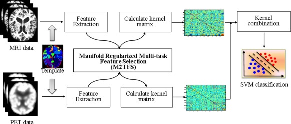
The proposed classification framework. [Color figure can be viewed in the online issue, which is available at http://wileyonlinelibrary.com.]
Subjects
The data used in the preparation of this article were obtained from ADNI database. The ADNI was launched in 2003 by the National Institute on Aging, the National Institute of Biomedical Imaging and Bioengineering, the Food and Drug Administration, private pharmaceutical companies, and nonprofit organizations, as a $60 million, 5‐year public–private partnership. The primary goal of ADNI has been to test whether the serial MRI, PET, other biological markers, and clinical and neuropsychological assessment can be combined to measure the progression of MCI and early AD. Determination of sensitive and specific markers of very early AD progression is intended to aid researchers and clinicians to develop new treatments and monitor their effectiveness, as well as lessen the time and cost of clinical trials.
ADNI is the result of efforts of many coinvestigators from a broad range of academic institutions and private corporations, and subjects have been recruited from over 50 sites across the US and Canada. The initial goal of ADNI was to recruit 800 adults, aged 55–90, to participate in the research—approximately 200 cognitively normal older individuals to be followed for 3 years, 400 people with MCI to be followed for 3 years, and 200 people with early AD to be followed for 2 years (see http://www.adni-info.org for up‐to‐date information). In current studies, we used a total of 202 subjects with corresponding baseline MRI and PET data, which includes 51 AD patients, 99 MCI patients (including 43 MCI converters and 56 MCI nonconverters), and 52 NC. Demographic information of the subjects is listed in Table 1. A detailed description on acquiring MRI, PET data from ADNI as used in this article can be found at [Zhang et al., 2011].
Table 1.
Characteristics of the subjects (mean ± standard deviation)
| AD (N = 51) | MCI (N = 99) | NC (N = 52) | |
|---|---|---|---|
| Age | 75.2 ± 7.4 | 75.3 ± 7.0 | 75.3 ± 5.2 |
| Education | 14.7 ± 3.6 | 15.9 ± 2.9 | 15.8 ± 3.2 |
| MMSE | 23.8 ± 1.9 | 27.1 ± 1.7 | 29.0 ± 1.2 |
| ADAS‐Cog | 18.3 ± 6.0 | 11.4 ± 4.4 | 7.4 ± 3.2 |
MMSE = Mini‐Mental State Examination, ADAS‐Cog = Alzheimer's Disease Assessment Scale‐Cognitive Subscale.
Image Preprocessing and Feature Extraction
Image preprocessing is performed for all MRI and FDG‐PET images. Specifically, we use the specific application tool for image preprocessing as similarly used in [Wang et al., 2014; Zhang et al., 2011], that is, spatial distortion, skull‐stripping, and removal of cerebellum. Then, for structural MR images, we use the FSL package [Zhang et al., 2001] to segment each image into three different tissues: gray matter (GM), white matter, and CSF. With atlas warping, each subject was partitioned into 93 ROIs [Shen and Davatzikos, 2002]. For each ROI, the volume of GM tissue in that ROI was computed as a feature. For FDG‐PET images, we use a rigid transformation to align it onto its respective MR image of the same subject, and then compute the average intensity of each ROI in the FDG‐PET image as a feature. Overall, by performing this series of image preprocessing, for each subject we can acquire 93 features from the MRI image and another 93 features from the PET image. We normalize the features of each modality with the same normalization scheme as used in [Zhang et al., 2011].
Manifold Regularized Multitask Feature Selection
Multitask learning aims to improve the performance of learning algorithms by jointly learning a set of related tasks [Argyriou et al., 2008; Obozinski et al., 2010], which is particularly useful when these tasks have some commonality and are generally slightly under sampled. Based on multitask learning framework, Zhang and Shen [2012] proposed a feature learning method to jointly predict the multiple regression and classification variables from multimodality data, and achieved state‐of‐the‐art performance in AD classification. Motivated by their work, we proposed a new multitask feature learning framework to jointly detect the disease‐related regions from multimodality data for classification. We first briefly introduce the existing multitask feature learning method. Then, we derive our manifold regularized multitask feature learning models, as well as the corresponding optimization algorithm.
Multitask feature selection
Assume that there are M supervised learning task (i.e., M modalities). Denote as the training data matrix in the m‐th task (i.e., m‐th modality) from N training subjects, and as the response vector from these training subjects, where represents the feature vector of the i‐th subject in the m‐th modality, and is the corresponding class label (i.e., patient or NC). It is worth noting that different modalities from the same subject have the same class label. Let wm ∈ Rd parameterize a linear discriminant function for task m. Then, the linear multitask feature selection (MTFS) model [Argyriou et al., 2008; Zhang and Shen, 2012] is to solve the following objective function:
| (1) |
where is the weight matrix whose row is the vector of coefficients associated with the j‐th feature across different tasks. Here, is the sum of the ‐norm of the rows of matrix W, as was used in the group‐sparsity regularizer [Yuan and Lin, 2006]. The use of ‐norm encourages the weight matrices with many zero rows. For feature selection, only those features with nonzero coefficients are kept. In other words, this norm combines multiple tasks and ensures that a small number of common features be jointly selected across different tasks. The parameter is a regularization parameter that balances the relative contributions of the two terms. The larger value means few features preserved for classification and vice versa. It is easy to show that the problem in Eq. (1) reduces to the ‐norm regularized optimization problem in the least absolution shrinkage and selection operator (LASSO) [Tibshirani, 1996] when the number of tasks equals to one.
Manifold regularized MTFS (M2TFS)
In the MTFS model, a linear mapping function (i.e., f(x) = wTx) was adopted to transform the data from the original high‐dimensional space to one‐dimensional space. In this model, for each task we only consider the relationship between data and class label, while the mutual dependence among data is ignored, which may result in large deviations even for very similar data after mapping. Figure 2 illustrates an example. Let's consider a pair of mapped data points y 1 and y 2 in Figure 2. Intuitively, these two points should be closer, as they come from the same class.
Figure 2.
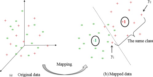
An example for illustrating the mutual dependence among data. [Color figure can be viewed in the online issue, which is available at http://wileyonlinelibrary.com.]
To address this issue, we introduced a new regularization item as:
| (2) |
where denotes a similarity matrix that defines the similarity on task m across different subjects. represents combinatorial Laplacian matrix for task m, where is the diagonal matrix defined as . Here, the similarity matrix is defined as:
| (3) |
This penalized item can be explained as follows: if and come from the same class, the distance between and should be smaller. It is easy to see that Eq. (2) aims to preserve the local neighboring structure of same‐class data during the mapping. With the regularizer in Eq. (2), the proposed manifold regularized MTFS model (M2TFS) has the following objective function:
| (4) |
where and are two positive constants. Their values can be determined via inner cross‐validation on the training data.
In our proposed M2TFS model, the group sparsity regularizer ensures only a small number of features to be jointly selected from multimodality data. The Laplacian regularization item preserves the discriminative information of the data from each modality via incorporating the label information of both classes and thus may induce more discriminative features.
Extension: Semisupervised M2TFS (semi‐M2TFS)
In general, semisupervised learning methods attempt to exploit the intrinsic data distribution disclosed by the unlabeled data and thus help construct a better learning model [Zhu and Goldberg, 2009]. In the proposed M2TFS model, we can redefine the similarity matrix in Eq. (2) to explore the geometric distribution information of original data for training a better learning model under semisupervised setting. Therefore, we extend our model to semisupervised version as follows.
We first define a diagonal matrix to indicate labeled and unlabeled data, that is, if the class label of subject i is unknown, and otherwise. Then, we redefine the similarity matrix with the following function:
| (5) |
where , and t is a free parameter to be tuned empirically. According to the redefinition of similarity matrix, we re‐explain the penalized item in Eq. (2) as follows: The more similarity between and , the distance between and should be smaller to minimize the objective function. Likewise, smaller similarity between and should lead to larger distance between and for minimization. According to this definition, it is easy to see that Eq. (2) preserve the geometric distribution information of the original data during the mapping. Finally, based on the formulation in Eq. (4), the objective function of our semisupervised M2TFS model (denoted as semi‐M2TFS) can be written as follows:
| (6) |
where is the corresponding Laplacian matrix, based on the newly defined similarity matrix in Eq. (5).Intuitively, the first term in Eq. (6) is for the supervised learning involving only the labeled data, while the last term in Eq. (6) involves both labeled and unlabeled data for unsupervised estimation on intrinsic geometric distribution of the whole data. It is worth noting that (i) Eq. (4) is a special case of Eq. (6), except for the definition of similarity matrix; (ii) the similarity matrix in Eq. (6) is defined purely by the distance in the original data space [i.e., given by Eq. (5)]. Below, we will develop a new method for optimizing the objective function in Eq. (6).
Optimization Algorithm
It is worth noting that, to the best of our knowledge, the objective function defined in Eq. (6) is the first to simultaneously include both the group‐sparsity and manifold regularizations, which cannot be solved by the existing sparse learning models. Accordingly, we resort to the widely used accelerated proximal gradient (APG) method [Beck and Teboulle, 2009; Chen et al., 2009; Liu and Ye, 2009]. Specifically, we first separate the objective function in Eq. (6) to a smooth part:
| (7) |
and a nonsmooth part:
| (8) |
Then, the following function is constructed for approximating the composite function :
| (9) |
where denotes the Frobenius norm, denotes the gradient of at point of the i‐th iteration, and l is the step size.
Finally, the update step of APG algorithm is defined as:
| (10) |
where and denote the j‐th row of the matrix W and V, respectively. Note that l can be determined by line search, and
| (11) |
Therefore, through Eq. (10), this problem can be decomposed into d separate subproblems. The key of APG algorithm is how to solve the update step efficiently. The study in [Chen et al., 2009; Liu and Ye, 2009] shows that the analytical solutions of those subproblems can be easily obtained:
| (12) |
In addition, according to a technique used in [Liu and Ye, 2009], instead of performing gradient descent based on , we compute the search point as:
| (13) |
where and .
The detailed optimization procedure is summarized in Algorithm 1. This algorithm achieves a convergence rate of and a time complexity of , where I is the maximum iteration. The detailed proof of convergence rate and also the time complexity of this algorithm are given in the Appendix.
Algorithm 1. (Semi‐)M2TFS.
Input: The data from training subjects, along with their corresponding response vector . For the case of semisupervised learning, for each unlabeled subject i. Output: Initialization: For i=1 to max_iteration I 1: Compute the search point according to Eq. (13) 2: 3: While ; Here is computed by Eq. (10). 4: Set End Calculate
CLASSIFICATION
Following [Zhang et al., 2011], we adopted the multikernel learning (MKL) SVM method for classification. Specifically, for each modality of training subjects, a linear kernel was first calculated based on the features selected by the above proposed method. Then, to combine multiple modality data, we adopted the following MKL technique:
| (14) |
where denotes the kernel function over the m‐th modality across subject x and z, and is a no‐negative weight parameter with .
In the current studies, the MKL technique used in [Zhang et al., 2011] was applied to combine multiple kernels. The optimal is determined based on the training subjects through a grid search with the range from 0 to 1 at a step size of 0.1, via another 10‐fold cross‐validation. Once the optimal was obtained, the standard SVM can be performed for classification.
RESULTS
To evaluate the effectiveness of our proposed method, we perform a series of experiments on the multimodality data from the ADNI database. Specifically, two sets of experiments, that is, supervised classification and semisupervised classification, were performed on 202 ADNI baseline MRI and PET data, respectively. In both sets of experiments, multiple binary classifiers, that is, AD versus NC, MCI versus NC, and MCI converters (MCI‐C) versus MCI nonconverters (MCI‐NC), are built, respectively. For classification, a linear SVM was implemented based on the LIBSVM library [Chang and Lin, 2001] with the default value for regularization parameter (i.e., C = 1). For evaluation of the proposed method, we adopt the classification accuracy, sensitivity, specificity, and area under receiver operating characteristic (ROC) curve (AUC) as performance measures. Here, the accuracy measures the proportion of subjects that are correctly predicted among all subjects, the sensitivity represents the proportion of patients that are correctly predicted, and the specificity denotes the proportion of NCs that are correctly predicted.
Supervised Classification
In this experiment, 10‐fold cross‐validation strategy was adopted to evaluate the classification performance. Specifically, the whole set of subject samples are divided into 10 equal portions, for each cross‐validation, the subject samples within one portion was left out for testing, and the remaining subject samples were used for training the classifier. This process is repeated for 10 times independently to avoid any bias introduced by randomly partitioning dataset in the cross‐validation, thereby yielding an unbiased estimate of classification error rate.
Classification performance
In the current studies, we compared our proposed method with the state‐of‐the‐art multi‐modality‐based methods, including MultiModality method proposed in [Zhang et al., 2011] (denoted as MM and MML, corresponding to the method without feature selection and the method using LASSO as feature selection, respectively) and MTFS method [Zhang and Shen, 2012] (denoted as MTFS). In addition, for more comparisons, we also concatenate all features from MRI and FDG‐PET into a long feature vector, and then perform three different feature selection methods, that is, t‐test, LASSO and sequential floating forward selection. Finally, the standard SVM with linear kernel was used for classification. The detailed experimental results are summarized in Table 2. Figure 3 plots the ROC curves of four multimodality‐based methods (i.e., MM, MML, MTFS, and the proposed method).
Table 2.
Classification performance of different methods
| Method | AD versus NC | MCI versus NC | MCI‐C versus MCI‐NC | |||||||||
|---|---|---|---|---|---|---|---|---|---|---|---|---|
| ACC (%) | SEN (%) | SPE (%) | AUC | ACC (%) | SEN (%) | SPE (%) | AUC | ACC (%) | SEN (%) | SPE (%) | AUC | |
| LASSO | 91.02 | 90.39 | 91.35 | 0.95 | 73.44 | 76.46 | 67.12 | 0.78 | 58.44 | 52.33 | 63.04 | 0.60 |
| t‐test | 90.94 | 91.57 | 90.00 | 0.97 | 73.02 | 78.08 | 63.08 | 0.77 | 59.11 | 53.49 | 63.57 | 0.64 |
| SFFS | 86.78 | 87.06 | 86.15 | 0.93 | 69.21 | 82.12 | 45.38 | 0.73 | 56.28 | 44.42 | 64.82 | 0.55 |
| MM | 91.65 | 92.94 | 90.19 | 0.96 | 74.34 | 85.35 | 53.46 | 0.78 | 59.67 | 46.28 | 69.64 | 0.60 |
| MML | 92.25 | 92.16 | 92.12 | 0.96 | 73.84 | 77.27 | 66.92 | 0.77 | 61.67 | 54.19 | 66.96 | 0.61 |
| MTFS | 92.07 | 91.76 | 92.12 | 0.95 | 74.17 | 81.31 | 60.19 | 0.77 | 61.61 | 57.21 | 65.36 | 0.62 |
| M2TFS | 95.03 | 94.90 | 95.00 | 0.97 | 79.27 | 85.86 | 66.54 | 0.82 | 68.94 | 64.65 | 71.79 | 0.70 |
ACC = ACCuracy, SEN = SENsitivity, SPE = SPEcificity.
Figure 3.
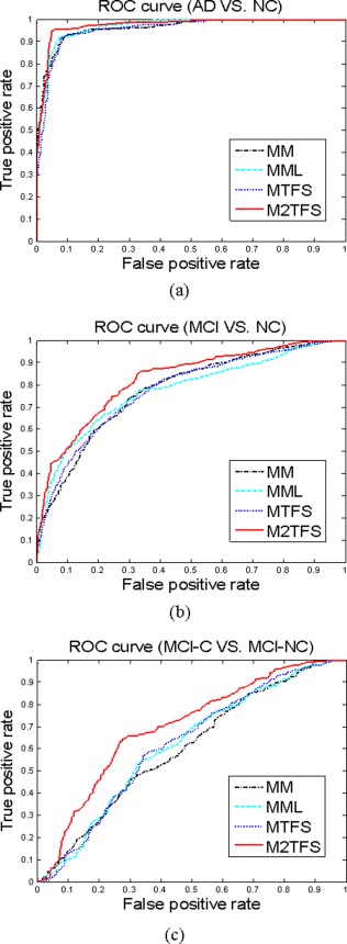
The ROC curves of four multimodality based methods. (a) the classification of AD vs. NC, (b) the classification of MCI versus NC, (c) the classification of MCI‐C versus MCI‐NC. [Color figure can be viewed in the online issue, which is available at http://wileyonlinelibrary.com.]
As we can see from Table 2 and Figure 3, our proposed M2TFS method consistently outperforms the other methods on three classification groups. Specifically, our proposed M2TFS method achieves the classification accuracy of 95.03, 79.27, and 68.94% for AD versus NC, MCI versus NC, and MCI‐C versus MCI‐NC, respectively, while the best classification accuracy of other methods are 92.25, 74.34, and 61.67%, respectively. Also, M2TFS is consistently superior to other methods in sensitivity measure. High sensitivity is very important for the purpose of diagnosis, because there are different costs for misclassifying a normal person to be a patient or misclassifying a patient to be a healthy person. Obviously, compared with the former, the latter may cause more severe consequences and thus has higher misclassification cost. Hence, it is advantageous for a classifier to provide higher sensitivity rate. In addition, the AUC of proposed method, respectively, is 0.97, 0.82, and 0.70 for those classifications, which indicates excellent diagnostic power. The results in Table 2 show that our proposed M2TFS method can take advantage of the local neighboring structure information of same‐class data to seek out the most discriminative subset of features. Besides, we performed the significance test between classification accuracy of our proposed and those of compared methods, using the standard paired t‐test. Table 3 gives the testing results, which show that our proposed method is significantly better than other feature selection methods (i.e., the corresponding p‐values are very small).
Table 3.
The significance test between the classification accuracies of our proposed method and other compared methods
| Compared method | P‐value | ||
|---|---|---|---|
| AD versus NC | MCI versus NC | MCI‐C versus MCI‐NC | |
| LASSO | <0.0001 | <0.0001 | 0.0010 |
| t‐test | <0.0001 | <0.0001 | 0.0063 |
| SFFS | <0.0001 | <0.0001 | 0.0004 |
| MM | <0.0001 | <0.0001 | 0.0019 |
| MML | 0.0009 | <0.0001 | 0.0062 |
| MTFS | <0.0001 | 0.0001 | 0.0086 |
Comparison of different combination schemes
To investigate the effect of combining weights, that is, and , on the performance of our multimodality classification method, we test all of their possible values, ranging from 0 to 1 at a step size of 0.1, with the constraint of . Figure 4 gives the classification performance, including classification accuracy and AUC value, on three classification groups with respect to different combining weights of MRI and PET. It is worth noting that, for each plot, the two vertices of the curve, that is, the leftmost and rightmost, denote the individual‐modality based results using only MRI ( ) and FDG‐PET ( ), respectively.
Figure 4.

The classification results on three classification groups with respect to different combining weights of MRI and PET (Left: classification accuracy; Right: AUC value). Note that µ PET + µ MRI = 1. [Color figure can be viewed in the online issue, which is available at http://wileyonlinelibrary.com.]
As we can see from Figure 4, most of inner intervals of the curve have larger values (i.e., better classification performance) than the two vertices, which indicate the effectiveness of combining two modalities for classification. Moreover, the intervals with higher performance mainly lie in a larger interval of [0.2, 0.8], implying that each modality is indispensable for achieving good classification performance. Further observation shows that this method is inferior to our adopted MKL‐based method as shown in Table 2, which implies that different modalities contribute differently and thus should be integrated adaptively for achieving better classification performance.
The most discriminative brain regions
It is of great interest to identify the biomarkers for disease diagnosis. With this consideration, in this subsection, we evaluated the discriminative power of the selected features (i.e., ROIs) using the proposed method. As the selected features are different in each cross‐validation, we choose these features with the highest selection frequency in all cross‐validation folds as the most discriminative features. For each selected discriminative feature, the standard paired t‐test was performed to evaluate its discriminative power between patients and controls groups. Table 4 lists the top 12 ROIs detected from both MRI and FG‐PET data for MCI classification. Figure 5 plots these regions in the template space. In addition, Table S1 and Table S2 in Supporting Information Appendix list the top ROIs selected for AD classification and MCI‐conversion classification, respectively.
Table 4.
Top 12 ROIs detected by our proposed M2TFS method for MCI versus NC classification
| Selected ROIs | MRI | FDG‐PET |
|---|---|---|
| L. cuneus | P = 0.0741 | P = 0.0626 |
| L. precuneus | P = 0.0001 | P = 0.0005 |
| L. temporal pole | P = 0.0004 | P = 0.0624 |
| L. entorhinal cortex | P < 0.0001 | P = 0.0286 |
| L. hippocampal formation | P < 0.0001 | P = 0.0109 |
| L. angular gyrus | P < 0.0001 | P = 0.0003 |
| R. hippocampal formation | P < 0.0001 | P = 0.0309 |
| R. occipital pole | P = 0.0375 | P = 0.8289 |
| L. occipital pole | P = 0.1638 | P = 0.0390 |
| R. amygdala | P < 0.0001 | P = 0.0352 |
| L. parahippocampal gyrus | P = 0.0009 | P < 0.0001 |
| R. precuneus | P = 0.0016 | P = 0.0007 |
L. = Left; R. = Right.
Figure 5.
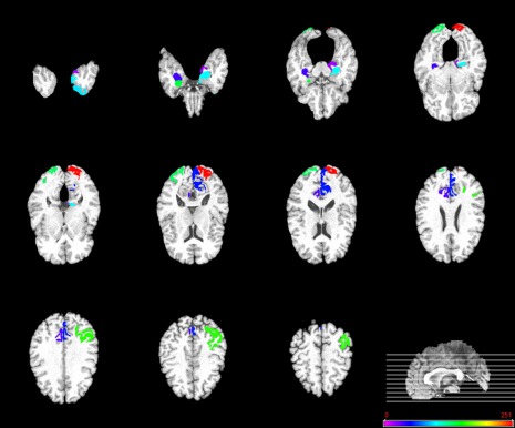
Top 12 ROIs detected by the proposed M2TFS method when performing MCI classification. [Color figure can be viewed in the online issue, which is available at http://wileyonlinelibrary.com.]
As can be seen from Table 4, most of the selected top regions for MCI classification, that is, hippocampus, amygdala, parahippocampus, temporal pole, precuneus, and entorhinal region, are consistent with the previous studies using group comparison [Del Sole et al., 2008; Derflinger et al., 2011; Nobili et al., 2008; Poulin et al., 2011; Solodkin et al., 2013; Wang et al., 2012; Wolf et al., 2003]. Also, from Supporting Information Table S1, we can see that most of the selected top regions for AD classification, that is, hippocampus, amygdala, temporal pole, precuneus, and uncus, are known to be related to AD by many studies using group comparison [Chetelat et al., 2002; Convit et al., 2000; Dai et al., 2009; Karas et al., 2007; Laakso et al., 2000]. A close observation on both Table 4 and Supporting Information Table S1 shows that some of the regions, that is, hippocampus, amygdala, temporal pole, and precuneus, are commonly selected for both classification tasks, which further indicates those brain regions may be much related to the AD. Conversely, most of selected features in Table 4 and Supporting Information Table S1 have very small P‐values, indicating their strong discriminative power in identifying AD/MCI patients from NCs.
Finally, Supporting Information Table S2 shows that some of the selected top regions for MCI‐conversion classification, that is, hippocampus, cingulated, and inferior frontal cortex, are also reported by the previous studies [Aksu et al., 2011; Drzezga et al., 2003; Ota et al., 2014]. However, most of the selected features in Supporting Information Table S2 are not as discriminative as the features obtained in AD/MCI classifications (in Table 4 and Supporting Information Table S1). This partly explains why lower performance is achieved in MCI‐conversion classification, compared to AD/MCI classifications.
Semisupervised Classification
In this subsection, we validate the effectiveness of proposed method under semisupervised setting. We first divided our subject samples into two portions: one portion is used as labeled data, and another portion is considered as unlabeled data; and then we performed two experiments to validate our proposed method from two aspects: (1) the classification performance with/without using unlabeled training subjects; (2) the performance of proposed method with different amounts of unlabeled training subjects.
In the first experiment, we first fixed a ratio r 1 = 50% of positive and negative subjects as labeled data. The rest of subjects were used as unlabeled data. We also adopted 10‐fold cross‐validation strategy to evaluate the classification performance. Specifically, for each cross‐validation, 90% of the labeled data together with the unlabeled data are used for training model. The rest of labeled data as well as the unlabeled data are used for testing the classification performance. This process is also repeated 10 times to avoid any bias introduced by randomly choosing labeled data. We also compared those feature selection methods as mentioned in supervised classification. Table 5 gives the classification performance of different methods.
Table 5.
The classification performance of different methods with 50% of labeled data
| Method | AD versus NC | MCI versus NC | MCI‐C versus MCI‐NC | |||||||||
|---|---|---|---|---|---|---|---|---|---|---|---|---|
| ACC (%) | SEN (%) | SPE (%) | AUC | ACC (%) | SEN (%) | SPE (%) | AUC | ACC (%) | SEN (%) | SPE (%) | AUC | |
| LASSO | 87.83 | 86.92 | 88.67 | 0.95 | 68.97 | 73.64 | 60.14 | 0.73 | 54.61 | 53.13 | 55.72 | 0.57 |
| t‐test | 88.60 | 90.85 | 86.41 | 0.96 | 72.12 | 80.53 | 56.19 | 0.75 | 55.34 | 51.16 | 58.48 | 0.57 |
| SFFS | 83.50 | 83.20 | 83.78 | 0.91 | 66.93 | 80.08 | 42.06 | 0.68 | 54.91 | 48.49 | 59.76 | 0.56 |
| MM | 87.55 | 89.49 | 85.64 | 0.94 | 71.47 | 86.87 | 42.30 | 0.73 | 57.47 | 46.80 | 65.43 | 0.58 |
| MML | 86.54 | 85.68 | 87.37 | 0.93 | 71.63 | 77.82 | 59.91 | 0.75 | 56.63 | 53.23 | 59.15 | 0.57 |
| MTFS | 87.63 | 86.90 | 88.30 | 0.94 | 71.62 | 79.91 | 55.91 | 0.73 | 56.52 | 50.03 | 61.39 | 0.56 |
| M2TFS | 89.25 | 85.80 | 92.59 | 0.95 | 73.03 | 89.39 | 42.03 | 0.75 | 58.38 | 55.69 | 60.26 | 0.58 |
| semi‐M2TFS | 90.38 | 90.91 | 89.73 | 0.95 | 75.06 | 84.71 | 56.78 | 0.77 | 60.57 | 47.74 | 70.23 | 0.61 |
ACC = ACCuracy, SEN = SENsitivity, SPE = SPEcificity.
From Table 5, we can observe that our proposed semi‐M2TFS method can further improve the performance compared with the supervised methods. Specifically, our proposed semi‐M2TFS method achieves the classification accuracy of 90.38, 75.06, and 60.57% for AD versus NC, MCI versus NC, and MCI‐C versus MCI‐NC, respectively, while the best classification accuracy of other methods are 89.25, 73.3, and 58.38%, respectively. In addition, the AUC of proposed method is 0.95, 0.77, and 0.61, respectively, for those classifications, which also indicates excellent diagnostic power. The results in Table 5 show that our proposed semi‐M2TFS method can take advantage of the geometric distribution information of original data (including labeled data and unlabeled data), and thus obtain a better learning model.
In the second experiment, we evaluate the performance of proposed method for different amounts of unlabeled training subjects. Specifically, we first fixed a ratio r 1 = 50% of positive and negative subjects as labeled data. In the following procedure, we used a fraction of the rest of subjects as unlabeled data. We evaluated our methods with selected labeled data and unlabeled data using 10‐fold cross‐validation. At each cross‐validation, 90% of the labeled data together with the unlabeled data are used for training model. The rest of labeled data as well as the unlabeled data are used for testing the classification performance. This process is also repeated 10 times independently. For any chosen fraction r 2 of unlabeled data, we also repeated 10 times to avoid any bias introduced by randomly choosing unlabeled data. The experiment is also repeated 10 times to avoid any bias introduced by randomly choosing labeled data. The average classification is computed for each fraction r 2. Figure 6 shows the classification accuracy of our proposed method with respect to different unlabeled samples.
Figure 6.
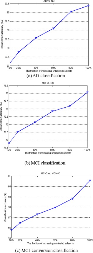
Classification accuracy with respect to the use of different number of unlabeled samples. [Color figure can be viewed in the online issue, which is available at http://wileyonlinelibrary.com.]
As we can see from Figure 6, the classification accuracy can be consistently improved with the increase of unlabeled samples on three classification groups, which again shows that the proposed method can lead to the selection of more discriminative features using geometric distribution of data, and as a result the classification performance is significantly improved with the increase of the number of unlabeled data. These results demonstrate the significant gain obtained using information of data distribution.
DISCUSSION
In this article, we have proposed a new multimodality based classification framework with two successive steps, that is, manifold regularized MTFS and multikernel SVM classification. Two different sets of experiments, that is, supervised classification and semisupervised classification, have been performed on 202 baseline subjects from ADNI to validate our proposed method. The results demonstrate that our proposed method can consistently and substantially improve the classification performance of the existing multimodality based classification method.
Significance of Results
Multimodality‐based classification methods have been used to fuse information from multiple different data source, as different imaging modalities can provide essential complementary information that can be used to enhance our understanding of brain disorders. A main aim of multimodality method is to access the joint information provided by multiple imaging technique, which in turn can be useful for identifying the dysfunctional regions implicated many brain disorders [Sui et al., 2012]. Recent emergence of multitask learning approach makes it possible to jointly identify and select features from different modalities. Our study demonstrated that, using multitask learning and embedding the distribution information of data, the proposed method can achieve a significantly improved performance for disease classification.
The regions involved in the course of AD/MCI classification by the proposed method are in agreement with previous studies. For example, hippocampal formation, which is thought to play an important role in memory, spatial navigation and control of attention, is one of the first brain regions to suffer damage with memory loss and disorientation. Researchers have found that the hippocampal formation is damaged heavily in AD, and is a focal point for pathology [Hyman et al., 1984; Van Hoesen and Hyman, 1990; Wolf et al., 2003]. The amygdala plays a primary role in the processing of memory, decision‐making and emotional reactions. Existing studies have shown this as another important subcortical region that is severely and consistently affected by pathology in AD [Dai et al., 2009; Knafo et al., 2009; Poulin et al., 2011]. In addition, group comparison based studies demonstrate significant abnormalities in parahippocampal gyrus [Solodkin et al., 2013; Wang et al., 2012], uncus [Laakso et al., 2000], temporal pole [Nobili et al., 2008], entorhinal cortex [Derflinger et al., 2011], precuneus [Del Sole et al., 2008; Karas et al., 2007], and angular [Hunt et al., 2006]. The fact that our results are consistent with the previous studies demonstrates that our proposed method can also help discover the disease‐related brain regions useful for disease diagnosis.
Multimodality Classification
Recent studies on AD and MCI have shown that biomarkers from different modalities contain complementary information for diagnosis of AD [Apostolova et al., 2010; Foster et al., 2007; Landau et al., 2010; Walhovd et al., 2010b]. Several studies on combining different modalities of biomarkers have been reported for multimodality classification [Bouwman et al., 2007; Chetelat et al., 2005; Fan et al., 2008a,b; Sokolova, 1991; Vemuri et al., 2009; Walhovd et al., 2010a; Wee et al., 2012; Yang et al., 2010], achieving better performance than baseline single‐modality methods. Two different strategies were often used in those methods, that is, (1) combining all features from different modalities into a longer feature vector for the following classification and (2) using MKL technique for multimodality data fusion and classification. Empirical results have shown that the latter often can achieve better classification performance than the former.
To evaluate the effect of combining multimodality data, we performed two additional experiments, that is, (1) using more modalities and (2) using only single modality. In the first experiment, besides MRI and PET modalities, we also included the CSF data (with Aβ42, t‐tau and p‐tau as features) using our proposed classification framework. Specifically, we combined three modalities data (i.e., MRI, FDG‐PET, and CSF) for classification [denoted as M2TFS (MRI+PET+CSF)]. While in the second experiment, for each modality, we performed LASSO‐based feature selection, and then used SVM with linear kernel for classification (denoted as MRI, PET and CSF, respectively). It is worth noting that feature selection was not necessary for CSF modality in both experiments. The corresponding experimental results are summarized in Table 6. Here, the proposed M2TFS with two modalities (i.e., MRI and FDG‐PET) is denoted as M2TFS (MRI+PET).
Table 6.
The classification performance with different modalities of data
| Method | AD versus NC | MCI versus NC | MCI‐C versus MCI‐NC | |||||||||
|---|---|---|---|---|---|---|---|---|---|---|---|---|
| ACC (%) | SEN (%) | SPE (%) | AUC | ACC (%) | SEN (%) | SPE (%) | AUC | ACC (%) | SEN (%) | SPE (%) | AUC | |
| PET | 84.42 | 83.53 | 84.81 | 0.91 | 67.11 | 75.96 | 50.19 | 0.72 | 54.44 | 48.37 | 59.11 | 0.57 |
| MRI | 88.68 | 84.51 | 92.50 | 0.94 | 73.12 | 78.28 | 63.65 | 0.79 | 52.22 | 44.19 | 58.21 | 0.54 |
| CSF | 82.26 | 82.55 | 81.54 | 0.87 | 70.72 | 71.62 | 69.04 | 0.75 | 58.72 | 53.02 | 63.04 | 0.63 |
| M2TFS (MRI+PET) | 95.03 | 94.90 | 95.00 | 0.97 | 79.27 | 85.86 | 66.54 | 0.82 | 68.94 | 64.65 | 71.79 | 0.70 |
| M2TFS (MRI+PET+CSF) | 95.38 | 94.71 | 95.77 | 0.98 | 82.99 | 89.39 | 70.77 | 0.84 | 72.28 | 66.05 | 76.61 | 0.72 |
ACC = ACCuracy, SEN = SENsitivity, SPE = SPEcificity.
As we can see from Table 6, our proposed method with three modalities [i.e., M2TFS (MRI+PET+CSF)] achieves the best classification performance, compared with that with two modalities [i.e., M2TFS (MRI+PET)] and those with single modality (i.e., PET, MRI, and CSF). Also, Table 6 shows that the performance of combining two modalities is better than that of using only single modality. These results further validate that different modalities of data contain complementary information, and the advantages of multimodality based methods over single‐modality based ones.
Conversely, in Table 7 we also compare our proposed method with the recent state‐of‐the‐art methods for multimodality based AD/MCI classification. As we can see from Table 7, compared with all other methods, our method achieves the best classification accuracy, which again validates the efficacy of our proposed method.
Table 7.
Comparison on classification accuracy of different multimodality classification methods
| Method | Subjects | Modalities | AD versus NC | MCI versus NC | MCI‐C versus MCI‐NC |
|---|---|---|---|---|---|
| (Hinrichs et al., 2011) | 48AD+66NC | MRI+PET | 87.6% | – | – |
| (Huang et al., 2011) | 49AD+67NC | MRI+PET | 94.3% | – | – |
| (Gray et al., 2013) | 37AD+75MCI(34MCI‐C+41MCI‐NC)+35NC | MRI+PET+CSF+genetic | 89.0% | 74.6% | 58.0% |
| (Liu et al., 2014) | 51AD+99MCI(43MCI‐C+56MCI‐NC)+52NC | MRI+PET | 94.4% | 78.8% | 67.8% |
| M2TFS | 51AD+99MCI(43MCI‐C+56MCI‐NC)+52NC | MRI+PET | 95.0% | 79.3% | 68.9% |
| M2TFS | 51AD+99MCI(43MCI‐C+56MCI‐NC)+52NC | MRI+PET+CSF | 95.4% | 83.0% | 72.3% |
In the current studies, multitask learning technique is used to learn a set of related features from multimodality data for improving the classification performance. As multitask learning can use the related auxiliary information among tasks, it often leads to a better learning model, compared to single‐task learning. Several studies have used multitask learning for disease classification and prediction. For example, Yuan et al. [2012] also used multitask learning framework for classification of incomplete multimodality of data. Zhang and Shen [2012] adopted multitask learning framework for joint prediction of multiple regression and classification variables. Zhou et al. [2013] formulated the prediction problem as a multitask regression problem by considering the prediction at each time point as a task. More recently, Liu et al. [2014] also adopted multitask feature learning framework for AD/MCI classification, by adding the intermodality constraint into its objective function. However, different from Liu et al.'s method, our proposed method simultaneously adopted group‐sparsity regularizer (for joint feature selection from multimodality data) and embed the distribution information of data into the learning model. The experimental results in Table 7 show that our method can achieve a better classification performance than Liu et al.'s method [Liu et al., 2014].
The Effect of Distinct Similarity Measures
In the proposed method, two different similarity measures are adopted, which are defined in Eqs. (3) and (5), respectively. The former was used to preserve the local neighboring structure of same‐class data during the mapping, while the latter was used to preserve the geometrical distribution information of original data. To evaluate the effects of both similarity measures, we perform two additional experiments. Specifically, in supervised setting, we first performed the proposed M2TFS method with the similarity defined in Eq. (5) (denoted as M2TFS‐S5), instead of the similarity defined in Eq. (3). Then, in semisupervised setting, we performed the proposed semi‐M2TFS method with a mixture of two similarity measures [i.e., the similarity between labeled data computed by Eq. (3), and the similarity computed by Eq. (5) for other cases] (denoted here as semi‐M2TFS‐Mix), instead of using the original similarity measure as defined in Eq. (5). Both experimental results are summarized in Tables 8 and IX, respectively. As we can see from both Tables 8 and IX, the M2TFS method achieves better performance than M2TFS‐S5 method, and semi‐M2TFS‐Mix method achieves better performance than semi‐M2TFS, which indicate that M2TFS and semi‐M2TFS‐Mix can both obtain more discriminative features (i.e., ROIs), as the similarity defined in Eq. (3) embeds the discriminative information of data.
Table 8.
The classification performance of the proposed M2TFS method with different similarity matrices
| Method | AD versus NC | MCI versus NC | MCI‐C versus MCI‐NC | |||||||||
|---|---|---|---|---|---|---|---|---|---|---|---|---|
| ACC (%) | SEN (%) | SPE (%) | AUC | ACC (%) | SEN (%) | SPE (%) | AUC | ACC (%) | SEN (%) | SPE(%) | AUC | |
| M2TFS | 95.03 | 94.90 | 95.00 | 0.97 | 79.27 | 85.86 | 66.54 | 0.82 | 68.94 | 64.65 | 71.79 | 0.70 |
| M2TFS‐S5 | 94.63 | 94.12 | 95.00 | 0.97 | 77.51 | 84.14 | 64.81 | 0.81 | 64.28 | 59.30 | 67.68 | 0.65 |
ACC = ACCuracy, SEN = SENsitivity, SPE = SPEcificity.
Table 9.
The classification performance of the proposed semi‐M2TFS method with different similarity matrices
| Method | AD versus NC | MCI versus NC | MCI‐C versus MCI‐NC | |||||||||
|---|---|---|---|---|---|---|---|---|---|---|---|---|
| ACC (%) | SEN (%) | SPE (%) | AUC | ACC (%) | SEN (%) | SPE (%) | AUC | ACC (%) | SEN (%) | SPE (%) | AUC | |
| semi‐M2TFS | 90.38 | 90.91 | 89.73 | 0.95 | 75.06 | 84.71 | 56.78 | 0.77 | 60.57 | 47.74 | 70.23 | 0.61 |
| semi‐M2TFS‐Mix | 91.03 | 91.32 | 90.63 | 0.96 | 75.42 | 85.60 | 56.11 | 0.78 | 60.83 | 50.88 | 68.32 | 0.62 |
ACC = ACCuracy, SEN = SENsitivity, SPE = SPEcificity.
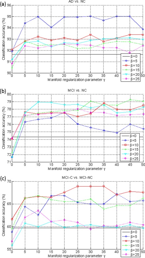
The Effect of Regularization Parameters
In our proposed M2TFS method, it includes two regularization items, that is, the group‐sparsity regularizer and the manifold regularization term. The parameters and balance the relative contribution of those regularization terms. To investigate the effects of the regularization parameters and on the classification performance of our proposed method, we test different values for , ranging from 0 to 25 at a step size of 5, and also test different values for , ranging from 0 to 50 at a step size of 5. Figure 7 shows the classification results with respect to different values of and . It is worth noting that, when , no feature selection step is performed, that is, all features extracted from MRI and FDG‐PET data are used for classification. So our method will be degraded to a multimodality method as proposed in [Zhang et al., 2011] (i.e., MM method). Also, when , no manifold regularization item is included, and thus our method will be degraded to a MTFS method.
Figure 7.
The classification accuracy with respect to the selection of γ and β. (a) AD classification, (b) MCI classification, and (c) MCI conversion classification. Each curve represents the performance for different selected value for β. X‐axis denotes for different values for γ. [Color figure can be viewed in the online issue, which is available at http://wileyonlinelibrary.com.]
As we can observe from Figure 7, under all values of and , our proposed M2TFS method consistently outperforms the MTFS methods on three classification groups (i.e., AD vs. NC, MCI vs. NC and MCI‐C vs. MCI‐NC), which further indicates the advantage of adding the manifold regularization term. Also, Figure 7 show that, when fixing the value of , the varied curves with the values of are very smooth on three classification groups, which shows that our method is very robust to the regularization parameter . Finally, we can see from Figure 7 that, when fixing the value of , the results on three classification groups are largely affected with different values of , which implies that the selection of is very important for the final classification results. This is reasonable as controls the sparsity of model and thus determines the size of the optimal feature subset.
Manifold Learning and Semisupervised learning
Manifold learning is a recent machine learning technique, which pursuits the goal to embed the original data in a high‐dimensional space into a lower dimensional space, while preserving the characteristic properties of the original data. As manifold learning enables dimensionality reduction and processing tasks in a meaningful lower‐dimensional space, it has been successfully applied to lots of tasks. In the community of machine learning, semisupervised learning based on manifold has been extensively studied and applied [Belkin and Niyogi, 2004; Zhu and Goldberg, 2009]. A few recent studies have applied manifold learning to medical imaging analysis [Aljabar et al., 2008; Guerrero et al., 2011; Wachinger and Navab, 2012; Wolz et al., 2012].
Semisupervised learning is a class of learning tasks that can make use of both labeled and unlabeled data for learning, where typically a small amount of labeled data with a large amount of unlabeled data are available. Existing studies have shown that a model can produce considerable improvement in learning performance when using unlabeled data together with a small amount of labeled data. The acquisition of labeled data is usually expensive and time‐consuming as it often requires a skilled human agent or a physical experiment, while the collection of unlabeled data is relatively easier. So, semisupervised learning is of great importance in practice. Among semisupervised learning methods, a promising family of techniques is to exploit the “manifold structure” of the data, which is generally based on the assumption that similar unlabeled subjects should be given the same classification [Zhu and Goldberg, 2009]. A few studies have applied semisupervised learning to medical imaging analysis [Dittrich et al., 2014]. For example, Filipovych and Davatzikos [2011] applied the semisupervised learning for classifying MCI subjects into MCI converters (MCI‐C) and MCI nonconverters (MCI‐NC) using semisupervised SVM method with 63 normal and 54 AD subjects as labeled data and 416 MCI subjects (including 242 MCI‐C and 174 MCI‐NC) as unlabeled data.
Conversely, in the proposed semi‐M2TFS method, we computed the classification performance on both the labeled data used for testing (i.e., testing data) and all the unlabeled data. However, in practice, it may be a better strategy to compute the classification accuracy using only the testing data (i.e., excluding all unlabeled data), as, for the latter, the training data and the testing data are completely independent, and thus the predictive model can be prelearned using the training data and then used directly to make prediction for the new subjects. Therefore, we recompute the classification accuracy using only the testing data, and the results show that our proposed method achieves the classification accuracy of 90.13, 74.99, and 60.04% for AD versus NC, MCI versus NC, and MCI‐C versus MCI‐NC, respectively, which are comparable to the corresponding results of semi‐M2TFS in Table 5. These results again validate the efficacy of our proposed method.
Limitation
The current study is limited by several factors. First, in the current study, we only investigated binary‐class classification problem (i.e., AD vs. NC, MCI vs. NC, and MCI‐C vs. MCI‐NC), but did not test the ability of the classifier for the multiclass classification of AD, MCI, and NCs. Second, the proposed method is based on multimodality data (i.e., FDG‐PET and MRI) and requires each subject having all corresponding modalities of data, which limits the size of subjects that can be used for study. Finally, other modalities of data (for example genetic data) can also be used for further improving the classification performance. In the future work, we will address the above limitations to further improve the performance of classification.
CONCLUSION
In summary, this article addresses the problem of exploiting the distribution information of data to build the multitask feature learning method for jointly selecting features from multimodalities of data. By introducing the manifold regularization term into the multitask learning framework, we used the APG algorithm to solve the optimal problem for seeking out the most informative feature subset. We have also developed the manifold regularized MTFS method for both supervised and semisupervised cases, with the corresponding algorithms denoted as M2TFS and semi‐M2TFS, respectively. Different from the existing MTFS methods, our method uses the distribution knowledge of data for early diagnosis of AD with better results. Experimental results on the ADNI dataset validate the efficacy of our proposed method.
Supporting information
Supplementary Information
ACKNOWLEDGMENTS
The grantee organization is the Northern California Institute for Research and Education, and the study is coordinated by the Alzheimer's Disease Cooperative Study at the University of California, San Diego. ADNI data are disseminated by the Laboratory for Neuron Imaging at the University of California, Los Angeles.
REFERENCES
- Aksu Y, Miller DJ, Kesidis G, Bigler DC, Yang QX (2011): An MRI‐derived definition of MCI‐to‐AD conversion for long‐term, automatic prognosis of MCI patients. PLoS One 6:e25074. [DOI] [PMC free article] [PubMed] [Google Scholar]
- Aljabar R, Rueckert D, Crum WR (2008): Automated morphological analysis of magnetic resonance brain imaging using spectral analysis. Neuroimage 43:225–235. [DOI] [PubMed] [Google Scholar]
- Apostolova LG, Hwang KS, Andrawis JP, Green AE, Babakchanian S, Morra JH, Cummings JL, Toga AW, Trojanowski JQ, Shaw LM, Jack CR, Jr , Petersen RC, Aisen PS, Jagust WJ, Koeppe RA, Mathis CA, Weiner MW, Thompson PM (2010): 3D PIB and CSF biomarker associations with hippocampal atrophy in ADNI subjects. Neurobiol Aging 31:1284–1303. [DOI] [PMC free article] [PubMed] [Google Scholar]
- Argyriou A, Evgeniou T, Pontil M 2008: Convex multi‐task feature learning. Machine Learn 73:243–272. [Google Scholar]
- Beck A, Teboulle M 2009: A fast iterative shrinkage‐thresholding algorithm for linear inverse problems. Siam J Imaging Sci 2:183–202. [Google Scholar]
- Belkin M, Niyogi P (2004): Semi‐supervised learning on Riemannian manifolds. Machine Learn 56:209–239. [Google Scholar]
- Bouwman FH, Schoonenboom SN, van der Flier WM, van Elk EJ, Kok A, Barkhof F, Blankenstein MA, Scheltens P (2007): CSF biomarkers and medial temporal lobe atrophy predict dementia in mild cognitive impairment. Neurobiol Aging 28:1070–1074. [DOI] [PubMed] [Google Scholar]
- Brookmeyer R, Johnson E, Ziegler‐Graham K, Arrighi HM (2007): Forecasting the global burden of Alzheimer's disease. Alzheimers Dement 3:186–191. [DOI] [PubMed] [Google Scholar]
- Chang CC, Lin CJ (2001): LIBSVM: a library for support vector machines.
- Chen X, Pan WK, Kwok JT, Carbonell JG (2009): Accelerated gradient method for multi‐task sparse learning problem. In: 9th IEEE International Conference on Data Mining, Florida, USA, pp 746–751.
- Chetelat G, Desgranges B, de la Sayette V, Viader F, Eustache F, Baron J‐C(2002): Mapping gray matter loss with voxel‐based morphometry in mild cognitive impairment. Neuroreport 13:1939–1943. [DOI] [PubMed] [Google Scholar]
- Chetelat G, Eustache F, Viader F, De La Sayette V, Pelerin A, Mezenge F, Hannequin D, Dupuy B, Baron JC, Desgranges B (2005): FDG‐PET measurement is more accurate than neuropsychological assessments to predict global cognitive deterioration in patients with mild cognitive impairment. Neurocase 11:14–25. [DOI] [PubMed] [Google Scholar]
- Chincarini A, Bosco P, Calvini P, Gemme G, Esposito M, Olivieri C, Rei L, Squarcia S, Rodriguez G, Bellotti R, Cerello P, De Mitri I, Retico A, Nobili F (2011): Local MRI analysis approach in the diagnosis of early and prodromal Alzheimer's disease. Neuroimage 58:469–480. [DOI] [PubMed] [Google Scholar]
- Convit A, de Asis J, de Leon MJ, Tarshish CY, De Santi S, Rusinek H, (2000): Atrophy of the medial occipitotemporal, inferior, and middle temporal gyri in non‐demented elderly predict decline to Alzheimer's disease. Neurobiol Aging 21:19–26. [DOI] [PubMed] [Google Scholar]
- Dai WY, Lopez OL, Carmichael OT, Becker JT, Kuller LH, Gach HM (2009): Mild cognitive impairment and Alzheimer disease: Patterns of altered cerebral blood flow at MR imaging. Radiology 250:856–866. [DOI] [PMC free article] [PubMed] [Google Scholar]
- Dai ZJ, Yan CG, Wang ZQ, Wang JH, Xia MR, Li KC, He Y (2012): Discriminative analysis of early Alzheimer's disease using multi‐modal imaging and multi‐level characterization with multi‐classifier (M3). Neuroimage 59:2187–2195. [DOI] [PubMed] [Google Scholar]
- Del Sole A, Clerici F, Chiti A, Lecchi M, Mariani C, Maggiore L, Mosconi L, Lucignani G, (2008): Individual cerebral metabolic deficits in Alzheimer's disease and amnestic mild cognitive impairment: An FDG PET study. Eur J Nucl Med Mol Imaging 35, 1357–1366. [DOI] [PubMed] [Google Scholar]
- Derflinger S, Sorg C, Gaser C, Myers N, Arsic M, Kurz A, Zimmer C, Wohlschlager A, Muhlau M (2011): Grey‐matter atrophy in Alzheimer's disease is asymmetric but not lateralized. J Alzheimers Dis 25:347–357. [DOI] [PubMed] [Google Scholar]
- Dittrich E, Riklin Raviv T, Kasprian G, Donner R, Brugger PC, Prayer D, Langs G (2014): A spatio‐temporal latent atlas for semi‐supervised learning of fetal brain segmentations and morphological age estimation. Med Image Anal 18:9–21. [DOI] [PubMed] [Google Scholar]
- Drzezga A, Lautenschlager N, Siebner H, Riemenschneider M, Willoch F, Minoshima S, Schwaiger M, Kurz A (2003): Cerebral metabolic changes accompanying conversion of mild cognitive impairment into Alzheimer's disease: A PET follow‐up study. Eur J Nucl Med Mol Imaging 30:1104–1113. [DOI] [PubMed] [Google Scholar]
- Fan Y, Resnick SM, Wu X, Davatzikos C (2008a): Structural and functional biomarkers of prodromal Alzheimer's disease: a high‐dimensional pattern classification study. Neuroimage 41:277–285. [DOI] [PMC free article] [PubMed] [Google Scholar]
- Fan Y, Batmanghelich N, Clark CM, Davatzikos C, Initia ADN (2008b); Spatial patterns of brain atrophy in MCI patients, identified via high‐dimensional pattern classification, predict subsequent cognitive decline. Neuroimage 39:1731–1743. [DOI] [PMC free article] [PubMed] [Google Scholar]
- Filipovych R, Davatzikos C (2011): Semi‐supervised pattern classification of medical images: application to mild cognitive impairment (MCI). Neuroimage 55:1109–1119. [DOI] [PMC free article] [PubMed] [Google Scholar]
- Foster NL, Heidebrink JL, Clark CM, Jagust WJ, Arnold SE, Barbas NR, DeCarli CS, Turner RS, Koeppe RA, Higdon R, Minoshima S (2007): FDG‐PET improves accuracy in distinguishing frontotemporal dementia and Alzheimer's disease. Brain 130:2616–2635. [DOI] [PubMed] [Google Scholar]
- Gray KR, Aljabar P, Heckemann RA, Hammers A, Rueckert D (2013): Random forest‐based similarity measures for multi‐modal classification of Alzheimer's disease. Neuroimage 65:167–175. [DOI] [PMC free article] [PubMed] [Google Scholar]
- Guerrero R, Wolz R, Rueckert D (2011): Laplacian Eigenmaps manifold learning for landmark localization in brain MR images. Med Image Comput Comput Assist Interv 14:566–573. [DOI] [PubMed] [Google Scholar]
- Higdon R, Foster NL, Koeppe RA, DeCarli CS, Jagust WJ, Clark CM, Barbas NR, Arnold SE, Turner RS, Heidebrink JL, Minoshima S (2004): A comparison of classification methods for differentiating fronto‐temporal dementia from Alzheimer's disease using FDG‐PET imaging. Stat Med 23:315–326. [DOI] [PubMed] [Google Scholar]
- Hinrichs C, Singh V, Mukherjee L, Xu G, Chung MK, Johnson SC (2009): Spatially augmented LPboosting for AD classification with evaluations on the ADNI dataset. Neuroimage 48:138–149. [DOI] [PMC free article] [PubMed] [Google Scholar]
- Hinrichs C, Singh V, Xu G, Johnson SC (2011): Predictive markers for AD in a multi‐modality framework: an analysis of MCI progression in the ADNI population. Neuroimage 55:574–589. [DOI] [PMC free article] [PubMed] [Google Scholar]
- Huang S, Li J, Ye J, Chen K, Wu T (2011): Identifying Alzheimer's disease‐related brain regions from multi‐modality neuroimaging data using sparse composite linear discrimination analysis. In Proceedings of Neural Information Processing Systems Conference, Granada, Spain.
- Hunt A, Schonknecht P, Henze M, Toro P, Haberkorn U, Schroder J (2006): CSF tau protein and FDG PET in patients with aging‐associated cognitive decline and Alzheimer's disease. Neuropsychiatr Dis Treat 2:207–212. [DOI] [PMC free article] [PubMed] [Google Scholar]
- Hyman BT, Hoesen GWV, Damasio AR, Barnes CL (1984): Alzheimer's disease: Cell‐specific pathology isolates the hippocampal formation. Science 225:1168–1170. [DOI] [PubMed] [Google Scholar]
- B Jie, D Zhang, W Gao, Q Wang, CY Wee, D Shen (2014a): Integration of network topological and connectivity properties for neuroimaging classification. IEEE Trans Biomed Eng 61:576–589. [DOI] [PMC free article] [PubMed] [Google Scholar]
- B Jie, D Zhang, CY Wee, D Shen (2014b): Topological graph kernel on multiple thresholded functional connectivity networks for mild cognitive impairment classification. Hum Brain Mapp 35:2876–2897. [DOI] [PMC free article] [PubMed] [Google Scholar]
- Karas G, Scheltens P, Rombouts S, van Schijndel R, Klein M, Jones B, van der Flier W, Vrenken H, Barkhof F (2007): Precuneus atrophy in early‐onset Alzheimer's disease: a morphometric structural MRI study. Neuroradiology 49:967–976. [DOI] [PubMed] [Google Scholar]
- Knafo S, Venero C, Merino‐Serrais P, Fernaud‐Espinosa I, Gonzalez‐Soriano J, Ferrer I, Santpere G, DeFelipe J (2009): Morphological alterations to neurons of the amygdala and impaired fear conditioning in a transgenic mouse model of Alzheimer's disease. J Pathol 219:41–51. [DOI] [PubMed] [Google Scholar]
- Laakso MP, Frisoni GB, Kononen M, Mikkonen M, Beltramello A, Geroldi C, Bianchetti A, Trabucchi M, Soininen H, Aronen HJ (2000): Hippocampus and entorhinal cortex in frontotemporal dementia and Alzheimer's disease: a morphometric MRI study. Biol Psychiatry 47:1056–1063. [DOI] [PubMed] [Google Scholar]
- Landau SM, Harvey D, Madison CM, Reiman EM, Foster NL, Aisen PS, Petersen RC, Shaw LM, Trojanowski JQ, Jack CR, Jr ., Weiner MW, Jagust WJ (2010): Comparing predictors of conversion and decline in mild cognitive impairment. Neurology 75:230–238. [DOI] [PMC free article] [PubMed] [Google Scholar]
- Liu F, Wee CY, Chen HF, Shen DG (2014): Inter‐modality relationship constrained multi‐modality multi‐task feature selection for Alzheimer's Disease and mild cognitive impairment identification. Neuroimage 84:466–475. [DOI] [PMC free article] [PubMed] [Google Scholar]
- Liu J, Ye J (2009): Efficient L1/Lq Norm Regularization. Technical report, Arizona State University.
- Liu M, Zhang D, Shen, D (2012): Ensemble sparse classification of Alzheimer's disease. Neuroimage 60:1106–1116. [DOI] [PMC free article] [PubMed]
- Ng B, Abugharbieh R (2011). Generalized sparse regularization with application to fMRI brain decoding. The 22rd biennial International Conference on Information Processing in Medical Imaging, Kloster Irsee, Germany, Vol. 22, pp 612–623. [DOI] [PubMed] [Google Scholar]
- Nobili F, Salmaso D, Morbelli S, Girtler N, Piccardo A, Brugnolo A, Dessi B, Larsson SA, Rodriguez G, Pagani M (2008): Principal component analysis of FDG PET in amnestic MCI. Eur J Nucl Med Mol Imaging 35:2191–2202. [DOI] [PubMed] [Google Scholar]
- Obozinski G, Taskar B, Jordan MI (2010): Joint covariate selection and joint subspace selection for multiple classification problems. Stat Comput 20:231–252. [Google Scholar]
- Oliveira PJ, Nitrini R, Busatto G, Buchpiguel C, Sato J, Amaro EJ (2010): Use of SVM methods with surface‐based cortical and volumetric subcortical measurements to detect Alzheimer's disease. J Alzheimers Dis 18:1263–1272. [DOI] [PubMed] [Google Scholar]
- Orru G, Pettersson‐Yeo W, Marquand AF, Sartori G, Mechelli A (2012): Using Support Vector Machine to identify imaging biomarkers of neurological and psychiatric disease: A critical review. Neurosci Biobehav Rev 36:1140–1152. [DOI] [PubMed] [Google Scholar]
- Ota K, Oishi N, Ito K, Fukuyama H (2014). A comparison of three brain atlases for MCI prediction. J Neurosci Methods 221:139–150. [DOI] [PubMed] [Google Scholar]
- Poulin SP, Dautoff R, Morris JC, Barrett LF, Dickerson BC, Initia ADN (2011): Amygdala atrophy is prominent in early Alzheimer's disease and relates to symptom severity. Psychiatry Res‐Neuroimaging 194:7–13. [DOI] [PMC free article] [PubMed] [Google Scholar]
- Shen D, Davatzikos C (2002): HAMMER: Hierarchical attribute matching mechanism for elastic registration. IEEE Trans Med Imaging 21:1421–1439. [DOI] [PubMed] [Google Scholar]
- Sokolova LV (1991): The specific spectral characteristics of the EEG of children with difficulties in learning to read. Fiziol Cheloveka 17:125–129. [PubMed] [Google Scholar]
- Solodkin A, Chen EE, Van Hoesen GW, Heimer L, Shereen A, Kruggel F, Mastrianni J (2013): In vivo parahippocampal white matter pathology as a biomarker of disease progression to Alzheimer's disease. J Comp Neurol 521:4300–4317. [DOI] [PubMed] [Google Scholar]
- Sui J, Adali T, Yu Q, Chen J, Calhoun VD (2012): A review of multivariate methods for multimodal fusion of brain imaging data. J Neurosci Methods 204:68–81. [DOI] [PMC free article] [PubMed] [Google Scholar]
- Tibshirani, R. , 1996. Regression shrinkage and selection via the Lasso. J R Stat Soc Ser B 58:267–288. [Google Scholar]
- Van Hoesen GW, Hyman BT (1990): Hippocampal formation: anatomy and the patterns of pathology in Alzheimer's disease. Prog Brain Res 83:445–457. [DOI] [PubMed] [Google Scholar]
- Vemuri P, Wiste HJ, Weigand SD, Shaw LM, Trojanowski JQ, Weiner MW, Knopman DS, Petersen RC, Jack CR Jr. (2009): MRI and CSF biomarkers in normal, MCI, and AD subjects: predicting future clinical change. Neurology 73, 294–301. [DOI] [PMC free article] [PubMed] [Google Scholar]
- Wachinger C, Navab N (2012). Entropy and Laplacian images: structural representations for multi‐modal registration. Med Image Anal 16;1–17. [DOI] [PubMed] [Google Scholar]
- Walhovd KB, Fjell AM, Brewer J, McEvoy LK, Fennema‐Notestine C, Hagler DJ, Jr ., Jennings RG, Karow D, Dale AM (2010a): Combining MR imaging, positron‐emission tomography, and CSF biomarkers in the diagnosis and prognosis of Alzheimer disease. AJNR Am J Neuroradiol 31:347–354. [DOI] [PMC free article] [PubMed] [Google Scholar]
- Walhovd KB, Fjell AM, Dale AM, McEvoy LK, Brewer J, Karow DS, Salmon DP, Fennema‐Notestine C (2010b): Multi‐modal imaging predicts memory performance in normal aging and cognitive decline. Neurobiol Aging 31:1107–1121. [DOI] [PMC free article] [PubMed] [Google Scholar]
- Wang C, Stebbins GT, Medina DA, Shah RC, Bammer R, Moseley ME, deToledo‐Morrell L (2012): Atrophy and dysfunction of parahippocampal white matter in mild Alzheimer's disease. Neurobiol Aging 33:43–52. [DOI] [PMC free article] [PubMed] [Google Scholar]
- Wang Y, Nie J, Yap PT, Li G, Shi F, Geng X, Guo L, Shen D (2014): Knowledge‐guided robust MRI brain extraction for diverse large‐scale neuroimaging studies on humans and non‐human primates. PLoS One 9:e77810. [DOI] [PMC free article] [PubMed] [Google Scholar]
- Wee CY, Yap PT, Zhang D, Denny K, Browndyke JN, Potter GG, Welsh‐Bohmer KA, Wang L, Shen D (2012): Identification of MCI individuals using structural and functional connectivity networks. Neuroimage 59:2045–2056. [DOI] [PMC free article] [PubMed] [Google Scholar]
- Westman E, Simmons A, Zhang Y, Muehlboeck JS, Tunnard C, Liu Y, Collins L, Evans A, Mecocci P, Vellas B, Tsolaki M, Kloszewska I, Soininen H, Lovestone S, Spenger C, Wahlund LO (2011): Multivariate analysis of MRI data for Alzheimer's disease, mild cognitive impairment and healthy controls. Neuroimage 54:1178–1187. [DOI] [PubMed] [Google Scholar]
- Wolf H, Jelic V, Gertz HJ, Nordberg A, Julin P, Wahlund LO (2003): A critical discussion of the role of neuroimaging in mild cognitive impairment. Acta Neurologica Scand 107:52–76. [DOI] [PubMed] [Google Scholar]
- Wolz R, Aljabar P, Hajnal JV, Lotjonen J, Rueckert D (2012): Nonlinear dimensionality reduction combining MR imaging with non‐imaging information. Med Image Anal 16:819–830. [DOI] [PubMed] [Google Scholar]
- Yang H, Liu J, Sui J, Pearlson G, Calhoun VD (2010): A hybrid machine learning method for fusing fMRI and genetic data: Combining both improves classification of Schizophrenia. Front Hum Neurosci 4:192. [DOI] [PMC free article] [PubMed] [Google Scholar]
- Ye JP, Wu T, Li J, Chen KW (2011): Machine learning approaches for the neuroimaging study of Alzheimer's Disease. Computer 44:99–101. [Google Scholar]
- Yuan M, Lin Y (2006). Model selection and estimation in regression with grouped variables. J R Stat Soc Ser B 68:49–67. [Google Scholar]
- Yuan L, Wang Y, Thompson PM, Narayan VA, Ye J (2012): Multi‐source feature learning for joint analysis of incomplete multiple heterogeneous neuroimaging data. Neuroimage 61:622–632. [DOI] [PMC free article] [PubMed] [Google Scholar]
- Zhang D, Shen D (2012). Multi‐modal multi‐task learning for joint prediction of multiple regression and classification variables in Alzheimer's disease. Neuroimage 59:895–907. [DOI] [PMC free article] [PubMed] [Google Scholar]
- Zhang Y, Brady M, Smith S (2001). Segmentation of brain MR images through a hidden Markov random field model and the expectation maximization algorithm. IEEE Trans Med Imaging 20:45–57. [DOI] [PubMed] [Google Scholar]
- Zhang D, Wang Y, Zhou L, Yuan H, Shen D (2011): Multimodal classification of Alzheimer's disease and mild cognitive impairment. Neuroimage 55:856–867. [DOI] [PMC free article] [PubMed] [Google Scholar]
- Zhou J, Liu J, Narayan VA, Ye J (2013): Modeling disease progression via multi‐task learning. Neuroimage 78:233–248. [DOI] [PubMed] [Google Scholar]
- Zhu X, Goldberg AB (2009) Introduction to semi‐supervised learning. San Rafael, Argentina: Morgan & Claypool.
Associated Data
This section collects any data citations, data availability statements, or supplementary materials included in this article.
Supplementary Materials
Supplementary Information