Towards A Magnetic Localization System for 3-D Tracking of Tongue Movements in Speech-Language Therapy

Abstract

This paper presents a new magnetic localization system based on a compact triangular sensor setup and three different optimization algorithms, intended for tracking tongue motion in the 3-D oral space. A small permanent magnet, secured on the tongue by tissue adhesives, will be used as a tracer. The magnetic field variations due to tongue motion are detected by a 3-D magneto-inductive sensor array outside the mouth and wirelessly transmitted to a computer. The position and rotation angles of the tracer are reconstructed based on sensor outputs and magnetic dipole equation using DIRECT, Powell, and Nelder-Mead optimization algorithms. Localization accuracy and processing time of the three algorithms are compared using one data set collected in which source-sensor distance was changed from 40 to 150 mm. Powell algorithm showed the best performance with 0.92 mm accuracy in position and 0.7^o in orientation. The average processing time was 43.9 ms/sample, which can satisfy real time tracking up to ~20 Hz.

I. Introduction

Aphasia is a neurological disorder that results from damage to portions of the brain that are responsible for language. These are often areas on the left hemisphere, which are shown in Fig. 1. The disorder impairs the expression and understanding of language as well as reading and writing. It may combine with speech disorders such as dysarthria or apraxia of speech, which also result from brain damage. In the U.S. alone, 80,000 new cases add every year to a total population of approximately one million, who suffer from aphasia. Aphasia usually occurs suddenly, often as a result of stroke or head injury, but it may also develop slowly, as in the case of a growing brain tumor, an infection, or dementia [1].

Fig. 1.

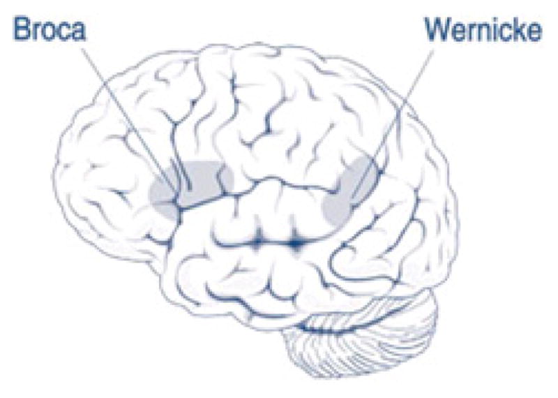
Areas of the brain affected by aphasia [1].

Aphasia therapy aims at improving the patients’ ability to communicate by helping them to use their remaining language abilities, and restore them as much as possible to compensate for other language problems. The patients also learn alternative methods of communication. Measuring the movements of the speech articulators such as the tongue with a high spatiotemporal resolution can be very helpful in the speech-language therapy by providing a quantitative visual representation of the tongue movements to the therapist and the patients, helping them to gain valuable insights into the nature of the speech disorder. However, it has been very difficult to access and measure the tongue motion in the oral cavity without impeding the patients’ natural speech, and this has hampered the study of the articulatory tongue motion.

Researchers have adopted real-time imaging techniques such as X-ray cinefluorography for measuring the tongue movements [2]. However, the harmful radiation exposure has precluded wide usage of this method. Ultrasound imaging of the tongue surface by scanning the soft tissue provides useful information about the shape of the tongue during speech [3]. However, accurate tracking of individual points of interest on the tongue such as the tip would be difficult. A safe and accurate alternative to imaging is tracking the tongue motion by alternating magnetic fields using small coils attached to the tongue. This method is known as electromagnetic articulography (EMA) [4]. However, the wires connected to each coil may interfere with speech, and the size and cost of the instrument are also quite high (> $100,000).

Our goal has been developing a small, robust, noninvasive, unobtrusive, and safe technology at low-cost and low power consumption that can accurately track and measure the tongue articulatory motion. Such a device should be easily usable in public and private clinical settings. It can even be utilized by the end users at home and educational environments for tongue training and exercising. The idea is to temporarily attach a small permanent magnetic tracer to the tongue, using tissue adhesives, and track the movements of the magnet inside the oral cavity by measuring the changes in the magnetic field, resulted from the tongue movements, with an array of magnetic sensors [5]. Because the size of the magnetic tracer (Ø5 mm × 1.5 mm) is much smaller than the distance between sensors and the oral space, it can be considered a magnetic dipole.

Several methods for magnetic dipole localization have been proposed. Yabukami et al. [6] measured the magnetic field by a pair of three-axial fluxgate sensors, and used the Powell technique for reconstructing the position and the orientation of a magnetic dipole [7]. Hashi et al. localized an LC magnetic marker with a resonant frequency of 175 kHz [8]. They measured the magnetic field distribution by a pickup coil array that consisted of 25 coils placed at intervals of 45 mm and determined the dipole parameters using the Gauss–Newton method. Wang et al. proposed to measure the magnetic field using 3-axis magnetoresistive sensors and performed a Levenberg-Marquardt optimization to fit the parameters of the magnetic tracer [10]. There are also commercial products that can localize multiple coils in 3-D space with high precision [11]. Nevertheless, occupying large volume and high power consumption deem all of these solutions unattractive for our tongue tracking application.

II. Magnetic Field Localization Theory

A. Mathematical Model of a Permanent Magnetic Dipole

Fig. 2 shows a cylindrical magnet with thickness l, diameter d, and residual magnetic strength B_r, at location a = (a_x, a_y, a_z). θ and γ are the zenith and azimuth angles, respectively, indicating the orientation of the dipole moment. The static magnetic flux density generated by this magnet, measured at a location s = (s_x, s_y, s_z), at a distance much larger than l and d, fits the dipole model given by

Fig. 2.

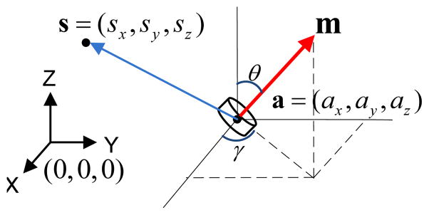
Vector representation of the magnetic dipole model.

$$\mathbf{B}(\mathbf{s},\mathbf{a},\mathbf{m})=\frac{{\mu }_0}{4\pi }\frac{3((\mathbf{s}-\mathbf{a})•\mathbf{m})(\mathbf{s}-\mathbf{a})-{\Vert \mathbf{s}-\mathbf{a}\Vert }^2\mathbf{m}}{{\Vert \mathbf{s}-\mathbf{a}\Vert }^5},$$ (1)

where m = [m·sin(θ)cos(γ), m·sin(θ)sin(γ), m·cos(θ)] is the magnetic moment vector of the dipole, and m =πB_rd²l/(4μ₀) is the magnitude of m [10], [12].

In order to localize the magnet, this 5 dimensional equation with five variables including three position variables (a_x, a_y and a_z) and two orientations (θ and γ) need to be solved. However, there is no closed form solution for this high order nonlinear equation. Therefore, iterative optimization method was chosen to estimate the position of the tracer based on the magnetic sensor output and dipole equation.

Assume a 3-axis sensor is at position s, with output vector of B_sensor, and a magnetic tracer is placed at position a. The magnetic field at the sensor position can be calculated using (1) based on an estimated magnetic tracer location and orientation. We define the mean square error between B_sensor and the magnetic flux density associated with the estimated magnet location, B, as the fitness function

$$F(a_x,a_y,a_z,\theta ,\gamma )=F({\mathbf{B}}_{\mathit{sensor}},\mathbf{B}(\mathbf{s},\mathbf{a},\mathbf{m}))=\Vert {\mathbf{B}}_{\text{sensor}}-\mathbf{B}(\mathbf{s},\mathbf{a},\mathbf{m})\Vert .$$ (2)

The smaller this five-variable fitness function is, the more accurate the estimated position and orientation will be.

B. Optimization Algorithms

Since calculating the partial derivatives of (2) are computationally intensive, we only choose optimization algorithms that solve difficult global optimization problems with real-valued fitness functions. These algorithms, which require no knowledge of the gradient of (2), are suitable to find the minimum value of (2) and find the parameter values at that point. In this paper, we employed three optimization algorithms: DIRECT, Nelder-Mead and Powell to find the minimum value of (2), and consequently the dipole location (a_x, a_y, a_z) and orientation (θ, γ).

1. DIRECT algorithm: “DIviding RECTangles” algorithm is a center-sampling strategy, which was developed by Jones et al. [9]. The goal in each step is to evaluate the midpoint of a domain, where lower and upper bounds are constructed. The domain is then trisected and two new center points are sampled in sub-domains that do not include the previous center point. At each iteration (dividing and sampling), DIRECT algorithm identifies intervals that contain the best fitness function values that are found up to that point. A disadvantage of this algorithm is that the boundaries cannot be reached. Hence, convergence to the global optimum will be slow if the global minimum lies at the boundary.

2. Nelder-Mead algorithm: is an unconstraint simplex method [13]. For (2), which has five unknown variables, the simplex is a 6-D shape with six vertices. This method is a pattern search that compares function values at these six vertices. The worst vertex, where F(a_x,a_y,a_z,θ,γ) is the largest, is rejected and replaced with a new vertex. A new 6-D shape is formed and the search is continued. The process generates a sequence of 6-D shapes (with different shapes), for which F(a_x,a_y,a_z,θ,γ) values get smaller and smaller. The size of the 6-D shape is reduced until the global minimum value of (2) is reached.

3. Powell algorithm [7]: Let X₀ be an initial guess for the five-variable location of the minimum of (2). An intuitive approach for approximating the minimum of (2) is to generate the next approximation, X₁, by proceeding successively to a minimum of F(a_x,a_y,a_z,θ,γ) along each of the 5 standard base vectors. Along each standard base vector, F is a function of only one variable, and it is easy to find its minimum. The process generates a sequence of points X₀ = P₀ → P₁ → P₂ → P₃ → P₄ → P₅. The vector P₅ – X₀ represents the average direction (from the beginning point to the end point) in each iteration. X₁ is determined along the vector P₅ – X₀ where the minimum of the function F occurs. At the end of this iteration, the first base vector is discarded and other base vectors shift to a lower vector, for P₅ X₀ to substitute the last base vector. This iteration is then repeated using the new set of direction vectors to generate a new sequence of points, and continues until the target minimum value of (2) is found.

III. System Overview

Our experimental setup for magnetic localization is shown in Fig. 3. A small disk shaped permanent magnet (Ø5 mm × 1.5 mm, weight = 0.21 g, B_r = 14500 G) (K&J, Jamison, PA) was used as the tracer and attached to a high spatial resolution 3-D Cartesian robot (VELMEX, Bloomfield, NY), which could be manually or automatically controlled from a graphical user interface (GUI) running on a PC. The robotic system can move the tracer in three orthogonal directions (x, y, z) in a range of 22 × 22 × 22 cm³ with 3.75 μm accuracy.

Fig. 3.

Experimental setup showing the positioning system and the GUI.

The flowchart of the tracking process is shown in Fig. 4, which includes four main steps: calibration, data recording, noise cancellation, and tracer localization.

Fig. 4.

Magnetic 3-D tracking flowchart.

Calibration

The purpose of calibration is to obtain the gain and DC offset of each magnetic sensor. In addition, the actual sensor positions within the robotic system coordinates should be accurately determined since the error in sensor position will eventually affect the accuracy of magnetic tracer localization. When the sensor array was setup, the same axes (X, Y and Z) of the sensors on different modules were aligned in parallel with their corresponding axes of the 3-D robotic system. Therefore, the orientation error of sensors was insignificant and did not need to be considered during the calibration process. Since the system is stationary after it is setup, the calibration step needs to be done only once.

Data Recording

Three 3-axial magneto-inductive sensor modules (PNI, Santa Rosa, CA) were placed 8 cm apart on the corners of an equilateral triangular Plexiglas board in the horizontal plane to capture the tracer magnetic field. An ultra low-power microcontroller (MSP430, Texas Instruments, Dallas, TX) took 13 samples/s from each sensor, while activating one sensor at a time to save power. The samples were packaged in a frame and wirelessly transmitted across a 2.4 GHz ISM-band wireless link, which was established between two identical low-power transceivers (nRF2401A, Nordic Semiconductor, Norway). The receiver was connected to the same PC that was used to control the robotic system and transferred the sensor data through a USB port.

Signal to noise ratio (SNR) of the measured data degrades when the distance between the tracer and sensor modules increases. Therefore, the moving space of the tracer was restricted within a virtual 9 × 9 × 4 cm³ cube.

Noise Cancellation

Even though the localization setup was stationary, the background noise, a combination of earth magnetic field (EMF) and adjacent DC magnetic sources, could slightly change over time. Therefore, before each localization the background magnetic field was measured and subtracted from the sensor outputs.

Tracer Localization

EMF-cancelled sensor outputs were converted to magnetic field strength using calibrated sensor gains and DC offsets. Then the optimization algorithms in Section II.B were used to find the best fit for 3-D position, a, and orientation (θ, γ) of the magnetic tracer.

In the optimization algorithms, the initial values of the five parameters (a_x0i,a_y0i,a_z0i,θ_0i,γ_0i) were set to zero. The first sample was always estimated by Nelder-Mead method and the following samples were reconstructed by three different algorithms. Besides, from the second sample on, the initial values of the searching parameters for the new sample were the estimated values of the previous sample,

$$(a_{\mathit{xNi}},a_{\mathit{yNi}},a_{\mathit{zNi}},{\theta }_{Ni},{\gamma }_{Ni})=(a_{xN-\mathit{1}},a_{yN-\mathit{1}},a_{zN-\mathit{1}},{\theta }_{N-\mathit{1}},{\gamma }_{N-\mathit{1}}).$$ (3)

Because Nelder-Mead and Powell algorithms are both unconstrained, there is no need to define a searching space for an incoming sample. However, DIRECT algorithm needs boundaries for each sample. The average speed of tongue movements during swallowing and speech is ~10.34 mm/s and it changes within 2.10 ~ 32.43 mm/s [17]. Considering that the sample rate of our system was 13 Hz, the spatial resolution should be at least 2.49 mm/sample, i.e. in order to capture all possible tracer movements, the bounds for DIRECT algorithm should be larger than 2.49 mm. Hence, in this paper, we set the search space for the new samples to be 5 mm and 10° for (a_x, a_y, a_z) and (θ, γ), respectively.

IV. Performance Evaluation

A. Spatial Accuracy and Processing Time

In order to evaluate the tracking performance of the system, the tracer was moved to a series of well defined positions by the 3-D robotic system and the difference with each localization algorithm output was calculated. After sensor calibration, the EMF was recorded before attaching the tracer. The tracer was attached to one end of a vertical dowel, which was mounted on the robotic arm, 2 cm lower from the tip. The robot moved the magnet within a 9 × 9 × 4 cm³ virtual cubic space with 1 cm intervals along each axis, resulting in a total of 10 × 10 × 5 measurements. The orientation of the magnet was held constant at θ = 90° and γ = 0° in this experiment. The collected data was subtracted by the EMF, and converted into magnetic field strength, and then fed into the localization algorithms.

Processing was done on a PC with 3.0 GHz Dual Core AMD processor with 3 GB RAM. Table I compares the performance of the three new algorithms and the Particle Swarm optimization (PSO) algorithm used in our prior work [14]. Because the search space and definition of error were different in [14], we recalculated them for PSO in Table I. It can be seen that the Powell algorithm can achieve the highest accuracy and the shortest processing time, suggesting that it is the prefer method for our future implementation. In addition, the 43.9 ms processing time makes it feasible to track the tongue motion, in real-time, with up to 20 samples/s.

Table I.

Localization Experiment Results

Algorithm	Position Error (mm)	Orientation Error (°)	Processing Time (msec/sample)
PSO	2.3	2.6	113.6
DIRECT	1.2	1.1	66.5
Nelder Mead	0.93	1.3	98.8
Powell	0.92	0.7	43.9

Table II benchmarks the performance of the present system among other previously reported magnetic tracking methods.

Table II.

Benchmarking of Magnetic Tracking Accuracy

Reference	Application	Space (cm)	Accuracy (mm/degree)		Number of Sensors
Hashi et al. [8]	Multi-motion capture	r = 10	<2	N/A	25 field coils
Wang et al. [10]	Capsule endoscope	Sphere r = 12	3.3	3	16 3-D sensors
Andra et al. [15]	Gastrointestinal motility	r = 20	10	N/A	3 field coils
Schlageter et al. [16]	Gastrointestinal motility	r = 14	<5	N/A	16 2-D sensors
This work	Tongue tracking	10×10×5	0.92	0.7	3 3-D sensors

B. Free Movement Tracking

In order to emulate the 3-D tongue tracking in a verifiable fashion, we moved the magnet by hand following pre-drawn trajectories on a tilted sheet of Plexiglas, placed over the sensor array (see Fig. 5). After data collection and noise cancellation, the Powell algorithm was used to reconstruct the trajectories. Fig. 5 shows a good match between the drawn and reconstructed 3-D patterns of “♡” and “g”.

Fig. 5.

Original and reconstructed 3-D trajectories

V. Conclusions

We have utilized three different algorithms to estimate 5 localization parameters of a small cylindrical magnetic tracer to be attached to the tongue. The spatiotemporal accuracy of the system and efficiency of the signal processing algorithm (Powell) were found to be sufficient for the intended application in real-time tracking of the tongue motion using a small, wireless, and low power system. Our future work will be focusing on the actual tongue tracking, and improving the signal processing algorithm for better temporal resolution. We will also work with speech-language therapists to utilize and evaluate our system in a clinical setting.

References

- 1.National Institute on Deafness and Other Communication Disorders, Voice, Speech, and Language, [online] Available: http://www.nidcd.nih.gov/health/voice.
- 2.Kent RD, Netsell R, Bauer LL. Cineradiographic assessment of articulatory mobility in the dysarthrias. Journal of Speech and Hearing Disorders. 1975 Nov;40:467–480. doi: 10.1044/jshd.4004.467. [DOI] [PubMed] [Google Scholar]
- 3.Shawker T, Sonies B, Stone M. Soft issue anatomy of the tongue and floor of the mouth: An ultrasound demonstration. Brain and Language. 1984 Mar;21:335–350. doi: 10.1016/0093-934x(84)90056-7. [DOI] [PubMed] [Google Scholar]
- 4.Schönle PW, Gräbe K, Wenig P, et al. Electromagnetic articulography: use of alternating magnetic fields for tracking movements of multiple points inside and outside the vocal tract. Brain and Language. 1987 May;31:26–35. doi: 10.1016/0093-934x(87)90058-7. [DOI] [PubMed] [Google Scholar]
- 5.Huo X, Wang J, Ghovanloo M. A magneto-inductive sensor based wireless tongue-computer interface. IEEE Trans on Neural Sys Rehab Eng. 2008 Oct;16(5):497–504. doi: 10.1109/TNSRE.2008.2003375. [DOI] [PMC free article] [PubMed] [Google Scholar]
- 6.Yabukami S, Kikuchi H, Arai KI, Takahashi K, Itagaki A, Wako N. Motion capture system of magnetic markers using three-axial magnetic field sensor. IEEE Trans Magn. 2000 Sep;36(5):3646–3648. [Google Scholar]
- 7.Powell MJD. An efficient method for finding the minimum of a function of several variables without calculating derivatives. The Computer Journal. 1964 Feb;7(2):155–162. [Google Scholar]
- 8.Hashi S, Tokunaga Y, Yabukami S, Kohno T, Ozawa T, Okazaki Y, Ishiyama K, Arai KT. Wireless motion capture system using magnetically coupled LC resonant marker. J Magn Magn Mater. 2005 Apr;290:1330–1333. [Google Scholar]
- 9.Jones DR, Perttunen CD, Stuckman BE. Lipschitzian optimization without the lipschitz constant. Journal of Optimization Theory and Application. 1993 Oct;79:157–181. [Google Scholar]
- 10.Wang X, Meng MQ, Hu C. A localization method using 3-axis magnetoresistive sensors for tracking of capsule endoscope. Proc Intl IEEE EMBS Conf. 2006 Aug;:2522–2525. doi: 10.1109/IEMBS.2006.260711. [DOI] [PubMed] [Google Scholar]
- 11.Liberty Latus, Polhemus Inc., [online] Available: http://www.polhemus.com/?page=Motion_Liberty_Latus.
- 12.Haynor DR, et al. System and method to determine the location and orientation of an indwelling medical device. 6263230. US Patent. 2001 Jul 17;
- 13.Nelder JA, Mead R. A simplex method for function minimization. Computer Journal. 1965;7:308–313. [Google Scholar]
- 14.Wang J, Huo X, Ghovanloo M. A Modified Particle Swarm Optimization Method for Real-Time Magnetic Tracking of Tongue Motion. Proc. IEEE 30th Eng. in Med. and Biol. Conf; Aug. 2008; [DOI] [PubMed] [Google Scholar]
- 15.Andra W, Danan H, Kirmbe W, Kramer HH, Saupe P, Schmieg R, Bellemann ME. A novel method for real-time magnetic marker monitoring in the gastrointestinal tract. Phys Med Biol. 2000;45:3081–3093. doi: 10.1088/0031-9155/45/10/322. [DOI] [PubMed] [Google Scholar]
- 16.Schlageter V, Besse PA, Popovic RS, Kucera P. Tracking system with five degrees of freedom using a 2D-array of Hall sensors and a permanent magnet. Sensors and Actuators A, Physical. 2001;92:37–42. [Google Scholar]
- 17.Peng CL, Jost-Brinkmann PG, Miethke RR, Lin CT. Ultrasonographic measurement of tongue movement during swallowing. Ultrasound Med. 2000;19:15–20. doi: 10.7863/jum.2000.19.1.15. [DOI] [PubMed] [Google Scholar]