Diagnostic classification of intrinsic functional connectivity highlights somatosensory, default mode, and visual regions in autism

Abstract

Despite consensus on the neurological nature of autism spectrum disorders (ASD), brain biomarkers remain unknown and diagnosis continues to be based on behavioral criteria. Growing evidence suggests that brain abnormalities in ASD occur at the level of interconnected networks; however, previous attempts using functional connectivity data for diagnostic classification have reached only moderate accuracy. We selected 252 low-motion resting-state functional MRI (rs-fMRI) scans from the Autism Brain Imaging Data Exchange (ABIDE) including typically developing (TD) and ASD participants (n = 126 each), matched for age, non-verbal IQ, and head motion. A matrix of functional connectivities between 220 functionally defined regions of interest was used for diagnostic classification, implementing several machine learning tools. While support vector machines in combination with particle swarm optimization and recursive feature elimination performed modestly (with accuracies for validation datasets <70%), diagnostic classification reached a high accuracy of 91% with random forest (RF), a nonparametric ensemble learning method. Among the 100 most informative features (connectivities), for which this peak accuracy was achieved, participation of somatosensory, default mode, visual, and subcortical regions stood out. Whereas some of these findings were expected, given previous findings of default mode abnormalities and atypical visual functioning in ASD, the prominent role of somatosensory regions was remarkable. The finding of peak accuracy for 100 interregional functional connectivities further suggests that brain biomarkers of ASD may be regionally complex and distributed, rather than localized.

Highlights

• •Machine learning of resting fMRI attains high diagnostic accuracy for autism.
• •Peak accuracy is seen for a complex pattern of 100 connectivities.
• •Somatosensory regions are overall most informative.
• •Default mode and visual regions also contribute to diagnostic accuracy.

1. Introduction

Autism spectrum disorder (ASD) is a highly heterogeneous disorder, diagnosed on the basis of behavioral criteria. From the neurobiological perspective, ‘ASD’ can be considered an umbrella term that may encompass multiple distinct neurodevelopmental etiologies (Geschwind and Levitt, 2007). Since any given cohort is thus likely composed of ill-understood subtypes (whose brain features may vary subtly or even dramatically), it is not surprising that brain markers with perfect sensitivity and specificity remain unavailable. Nonetheless, given the specificity of diagnostic criteria (American Psychiatric Association, 2013), the hope that some (potentially complex) patterns of brain features may be unique to the disorder is not unreasonable and worthy of pursuit.

Issues of heterogeneity and cohort effects can be partially addressed through the use of large samples, as provided by the recent Autism Brain Imaging Data Exchange (ABIDE) (Di Martino et al., 2014), which incorporates over 1100 resting state functional MRI (rs-fMRI) datasets from 17 sites. The use of these data for examining functional connectivity matrices for large numbers of ROIs across the entire brain is further promising, as there is growing consensus about ASD being characterized by aberrant connectivity in numerous functional brain networks (Schipul et al., 2011; Vissers et al., 2012; Wass, 2011). However, the functional connectivity literature in ASD is complex and often inconsistent (Müller et al., 2011; Nair et al., 2014), and data-driven machine learning (ML) techniques provide valuable exploratory tools for uncovering potentially unexpected patterns of aberrant connectivity that may characterize the disorder.

A few previous ASD studies have used intrinsic functional connectivity MRI (fcMRI) (Van Dijk et al., 2010) for diagnostic classification, i.e., for determining whether a dataset is from an ASD or typically developing participant solely based on functional connectivity. Anderson and colleagues (2011), using a large fcMRI connectivity matrix, reached an overall diagnostic classification accuracy of 79%, which was however lower in a separate small replication sample. Uddin et al. (2013a) used a logistic regression classifier for 10 rs-fMRI based features identified by ICA, which corresponded to previously described functional networks. The classifier achieved accuracies about 60–70% for all but one component identified as salience network, for which accuracy reached 77%. Imperfect accuracy in these studies may be attributed to moderate sample sizes (N ≤ 80). However, in a recent classification study using the much larger ABIDE dataset, Nielsen et al. (2013) reported an overall accuracy of only 60%, suggesting that the approach selected, a leave-one-out classifier using a general linear model, may not be sufficiently powerful.

In the present study, we implemented several multivariate learning methods, including random forest (RF), which is an ensemble learning method that operates by constructing many individual decision trees, known in the literature as classification and regression trees (CART). Each decision tree in the forest makes a classification based on a bootstrap sample of the data and a random subset of the input features. The forest as a whole makes a prediction based on the majority vote of the trees. One desirable feature of the random forest algorithm is the bootstrapping of the sample to have a built-in training and validation mechanism, generating an unbiased out-of-bag error that measures the predictive power of the forest. Features were intrinsic functional connectivities (Van Dijk et al., 2010) between a standard set of regions of interest using only highest quality (low motion) datasets from ABIDE.

2. Methods and materials

Data were selected from the Autism Brain Imaging Data Exchange (ABIDE, http://fcon_1000.projects.nitrc.org/indi/abide/) (Di Martino et al., 2013), a collection of over 1100 resting-state scans from 17 different sites. In view of the sensitivity of intrinsic fcMRI analyses to motion artifacts and noise (as described below), we prioritized data quality over sample size. We excluded any datasets exhibiting artifacts, signal dropout, suboptimal registration or standardization, or excessive motion (see details below). Sites acquiring fewer than 150 time points were further excluded. Based on these criteria, we selected a subsample of 252 participants with low head motion (see details below). Groups were matched on age and motion to yield a final sample of 126 TD and 126 ASD participants, ranging in age from 6 to 36 years (see Table 1 for summary and see Inline Supplementary Table S1 for fully detailed participant and site information).

Table 1.

Participant information.

Full sample	ASD, M ± SD [range, #391]	TD, M ± SD [range, #391]	p-Value (2-sample t-test)
N (female)	126 (18)	126 (31)
Age (years)	17.311 ± 6.00 [8.2–35.7]	17.116 ± 5.700 [6.5–34]	0.800
Motion (mm)	.057 ± .020 [.018–.108]	.058 ± .020 [.020–.125]	0.923
Non-verbal IQ	106.86 ± 17.0 [37–149]	106.28 ± 12.8 [67–155]	0.800

Inline Supplementary Table S1.

Table S1.

ABIDE demographic information.

Sites	Sample Size		Age		RMSD		NVIQ		Gender		ADOS_total		Handedness
	ASD	TD	ASD	TD	ASD	TD	ASD	TD	Male	Female	Range	NA	Left	Right
			mean (SD)		mean (SD)		mean (SD)
			[range]		[range]		[range]		[range]
FULL SAMPLE
NYU (N=70)	36	34	15.6 (6)	16.96 (6.17)	.02 (.02)	.02 (.02)	108 (15.1)	103 (14.9)	54	16	[5-22]	0	NA	NA
			[8.5-30]	[6.4-30.8]	[.03-.09]	[.03-.09]	[72-149]	[67-137]
UM_1 (N=29)	15	14	14.7 (2.1)	15.5 (2.8)	.06 (.02)	.05 (.02)	112 (19.6)	102.2 (9.4)	17	12	NA	15	5	21
			[11.5-18.6]	[11-19]	[.02-.09]	[.02-.08]	[81-148]	[82-113]
USM (N=29)	19	20	21.9 (6.4)	6.4 (7.2)	.05 (.02)	.06 (.02)	105.7 (13)	111 (12.5)	29	0	[6-21]	0	NA	NA
			[11.3-35.7]	[13.8-34]	[.02-.09]	[.03-.09]	[75-133]	[90-129]
SDSU (N=25)	10	15	14.6 (2.3)	13.4 (2.3)	.03 (.01)	.04 (.02)	112 (16)	111 (11)	21	4	[4-17]	0	6	19
			[9.6-17.7]	[8-16.8]	[.02-.05]	[.02-.07]	[86-114]	[92-137]
Leuven_1 (N=17)	9	8	22.2 (4.9)	23.75 (2.9)	.061 (.02)	.065 (.02)	103 (16.4)	114 (18.9)	17	0	NA	9	1	16
			[19-32]	[21-29]	[.04-.09]	[.04-.09]	[74-120]	[93-155]
Leuven_2 (N=17)	8	9	13.8 (1.1)	14.3 (1.4)	.07 (.01)	.08 (.02)	97.5 (11.8)	101.4 (6.5)	11	6	NA	8	4	13
			[12.2-15.3]	[12.3-16.6]	[.05-.1]	[.05-.1]	[83-117]	[89-109]
PITT (N=14)	8	6	21.2 (8.4)	20.2 (4.1)	.07 (.02)	.09 (.02)	11.7 (14.2)	115 (5.3)	12	2	[7-19]	1	1	13
			[12.6-35.2]	[12.8-24.6]	[.04-.1]	[.07-.1]	[93-128]	[108-121]
TRINITY (N=12)	4	8	17.2 (3.4)	17.9 (4)	.06 (.010)	.07 (.01)	121 (7.4)	111 (6.2)	12	0	[7-15]	0	0	12
			[13.6-20.8]	[12.7-24.8]	[.05-.07]	[.06-.07]	[114-131]	[103-121]
YALE (N=12)	6	6	14.6 (1.9)	13.2 (3.4)	.06 (.02)	.05 (.01)	85 (29)	97 (11.2)	8	4	NA	5	1	11
			[11.8-17.2]	[8.7-16.7]	[.03-.09]	[.03-.06]	[37-120]	[84-115]
KKIN (N=8)	3	5	9.9 (1.51)	9.9 (1.7)	.01 (.004)	.01 (.02)	NA	NA	6	2	[10-16]	0	1	7
			[8.2-11.1]	[8.5-12.8]	[.06-.07]	[.05-.1]
OLIN (N=8)	4	4	18.3 (4.03)	19.5 (2.4)	.09 (.01)	.09 (.3)	NA	NA	6	2	[7-19]	4	0	8
			[15-24]	[16-21]	[.07-.1]	[.06-.1]
UM_2 (N=6)	1	5	17.4 (NA)	18.4 (5.9)	.08 (NA)	.05 (.01)	80 (NA)	102 (6.8)	6	0	NA	1	0	6
			[17.4-17.4]	[14.5-28.9]	[.08-.08]	[.03-.06]	[80-80]	[92-109]
CMU (N=5)	3	2	26.7 (4.5)	26 (.07)	.06 (.02)	.08 (.01)	113.7 (10.8)	109.5 (0.7)	4	1	[8-16]	0	0	5
			[22-31]	[21-31]	[.04-.07]	[.07-.08]	[106-126]	[109-110]
TRAINING
NYU (N=60)	31	29	15.96 (6.22)	16.96 (6.50)	.05 (.02)	0.05 (0.02)	108.03 (15.80)	102.93 (15.17)	46	14	[6-22]	29	NA	NA
			[8.51 - 29.98]	[6.47 - 30.78]	[.03 -.09]	[0.03 - 0.09]	[72.00 - 149.00]	[67.00 - 137.00]
UM_1 (N=25)	14	11	14.64 (2.11)	15.28 (2.85)	0.06 (0.02)	0.05 (0.02)	111.43 (19.97)	105.11 (6.72)	15	10	NA	14	5	17
			[11.50 - 18.60]	[11.00 - 19.20]	[0.02 - 0.09]	[0.02 - 0.08]	[81.00 - 148.00]	[92.00 - 113.00]
Leuven_1 (N=17)	9	8	22.22 (4.87)	23.75 (2.92)	0.06 (0.02)	0.07 (0.02)	103.00 (16.42)	113.88] (18.88)	17	0	NA	9	1	16
			[19.00 - 32.00]	[21.00 - 29.00]	[0.04 - 0.09]	[0.04 - 0.09]	[74.00 - 120.00]	[93.00 - 155.00
SDSU (N=17)	9	8	15.19 (1.65)	13.43 (3.35)	0.03 (0.01)	0.04 (0.01)	112.67 (16.77)	110.25 (13.61)	17	0	[4-17]	0	5	12
			[12.88 - 17.67]	[8.02 - 16.59]	[0.02 - 0.05]	[0.02 - 0.07]	[86.00 - 140.00]	[92.00 - 137.00]
USM (N=16)	8	8	23.67 (7.35)	21.60 (6.84)	0.05 (0.02)	0.06 (0.02)	101.75 (6.82)	111.38 (13.22)	16	0	[9-17]	0	NA	NA
			[15.85 - 35.71]	[13.81 - 34.01]	[0.02 - 0.07]	[0.03 - 0.09]	[87.00 - 106.00]	[90.00 - 129.00]
Leuven_2 (N=14)	6	8	13.53 (1.23)	14.59 (1.32)	0.07 (0.01)	0.07 (0.01)	96.17 (9.54)	102 (6.70)	8	6	NA	6	3	11
			[12.20 - 15.30]	[12.30 - 16.60]	[0.05 - 0.08]	[0.05 - 0.10]	[83.00 - 106.00]	[89.00 - 109.00]
PITT (N=11)	6	5	23.03 (9.07)	20.01 (4.56)	0.08 (0.02)	0.09 (0.01)	114.67 (14.90)	114.20 (5.07)	10	1	[7-19]	1	1	10
			[12.62 - 35.20]	[12.83 - 24.60]	[0.06 - 0.11]	[0.07 - 0.11]	[93.00 - 128.00]	[108.00 - 119.00]
YALE (N=9)	4	5	14.96 (2.39)	12.53 (3.30)	0.07 (0.02)	0.04 (0.01)	84.75 (37.03)	98.20 (12.32)	8	1	NA	3	1	8
			[11.83 - 17.17]	[8.67 - 16.66]	[0.04 - 0.09]	[0.03 - 0.06]	[37.00 - 120.00]	[84.00 - 115.00]
KKI (N=8)	3	5	9.88 (1.51)	9.91 (1.69)	0.07 (0.00)	0.07 (0.02)	NA	NA	6	2	[10-16]	0	1	7
			[8.20 - 11.14]	[8.46 - 12.76]	[0.06 - 0.07]	[0.05 - 0.10]
OLIN (N=7)	3	4	18.3 (4.93)	19.50 (2.38)	0.09 (0.01)	0.09 (0.03)	NA	NA	5	2	[9-19]	0	0	7
			3[15.00 - 24.00]	[16.00 - 21.00]	[0.08 - 0.10]	[0.06 - 0.13]
TRINITY (N=7)	3	4	16.46 (3.79)	19.48 (4.53)	0.06 (0.01)	0.06 (0.01)	123.00 (7.21)	112.00 (6.38)	7	0	[7-15]	0	0	7
			[13.58 - 20.75]	[13.75 - 24.83]	[0.05 - 0.07]	[0.06 - 0.08]	[117.00 - 131.00]	[107.00 - 121.00]
CMU (N=5)	3	2	26.67 (4.51)	26.00 (7.07)	0.06 (0.02)	0.08 (0.01)	113.67 (10.79)	109.50 (0.71)	4	1	[8-16]	0	0	5
			[22.00 - 31.00]	[21.00 - 31.00]	[0.04 - 0.08]	[0.07 - 0.08]	[106.00 - 126.00]	[109.00 - 110.00]
UM_2 (N=4)	1	3	17.40 (0.00)	15.23 (0.67)	0.08 (0.00)	0.04 (0.02)	80.00 (0.00)	99.33 (7.02)	4	0	NA	1	0	4
			[17.40 - 17.40]	[14.50 - 15.80]	[0.08 - 0.08]	[0.03 - 0.06]	[80.00 - 80.00]	[92.00 - 106.00]
VALIDATION
USM (N=13)	11	2	20.7 (5.7)	28.2 (5.6)	.05 (.02)	.06 (.005)	105.9 (17.9)	109.5 (11.3)	12	1	[6-21]	1	NA	NA
			[11.4-32.8]	[22-34]	[.03-.09]	[.05-.07]	[75-133]	[100-119]
NYU (N=10)	5	5	13.1 (3.99)	16.4 (4.3)	.07 (.02)	.05 (.01)	38.8 (11.5)	102.8 (14.7)	2	8	[5-13]	0	NA	NA
			[8.9-17.9]	[9.8-20.0]	[.04-.09]	[.03-.06]	[92-119]	[83-117]
SDSU (N=8)	1	7	9.64	13.5 (2.9)	0.025	.04 (.018)	112	111.7 (8.3)	4	4	11	0	1	7
				[9.6-16.8]		[.02-.07]		[103-124]
TRINITY (N=5)	1	4	19.4	16.3 (3.2)	0.057	.066 (.0087)	114	109.8 (6.7)	5	0	13		0	5
				[12.7-20.1]		[.05-.076]		[103-116]
UM_1 (N=4)	1	3	16.1	16.2 (2.7)	0.048	.05 (.01)	125	178 (9.9)	2	2	NA	1	0	4
				[13.1-18.2]		[.03-.06]		[82-96]
Leuven_2 (N=3)	2	1	14.5 (.29)	12.4	.08 (.02)	0.11	101.5 (21.9)	97	3	0	NAN	3	1	2
			[14.3-14.7]		[.07-.09]		[86-117]
PITT (N=3)	2	1	15.6 (1.9)	21.22	.05 (.03)	0.11	103 (9.9)	121	2	1	[12-16]	0	0	3
			[14.2-16.9]		[.03-.07]		[96-110]
YALE (N=3)	2	1	14 (0.53)	16.66	.049 (.02)	0.057	85 (1.4)	93	0	3	NA	2	0	3
			[13.66-14.4]		[.03-.06]		[84-86]
UM_2 (N=2)	0	2	NA	23.2 (7.9)	NA	.06 (.003)	NA	107.5 (2.2)	2	0	NA	NA	0	2
				[17.6-28.8]		[.058-.06]		[106-109]
OLIN (N=1)	1	0	18	NA	0.07	NA	NA	NA	1	0	7	0	0	1

Data were selected from the Autism Brain Imaging Data Exchange (ABIDE, http://fcon_1000.projects.nitrc.org/indi/abide/) (Di Martino et al., 2013), a collection of over 1100 resting-state scans from 17 different sites. In view of the sensitivity of intrinsic fcMRI analyses to motion artifacts and noise (as described below), we prioritized data quality over sample size. We excluded any datasets exhibiting artifacts, signal dropout, suboptimal registration or standardization, or excessive motion (see details below). Sites acquiring fewer than 150 time points were further excluded. Based on these criteria, we selected a subsample of 252 participants with low head motion (see details below). Groups were matched on age and motion to yield a final sample of 126 TD and 126 ASD participants, ranging in age from 6 to 36 years (see Table 1 for summary and see Inline Supplementary Table S1 for fully detailed participant and site information).

Inline Supplementary Table S1 can be found online at http://dx.doi.org/10.1016/j.nicl.2015.04.002.

2.1. Data preprocessing

Data were processed using the Analysis of Functional NeuroImages software (Cox, 1996) (http://afni.nimh.nih.gov) and FSL 5.0 (Smith et al., 2004) (http://www.fmrib.ox.ac.uk/fsl). Functional images were slice-time corrected, motion corrected to align to the middle time point, field-map corrected and aligned to the anatomical images using FLIRT with six degrees of freedom. FSL's nonlinear registration tool (FNIRT) was used to standardize images to the MNI152 standard image (3 mm isotropic) using sinc interpolation. The outputs were blurred to a global full-width-at-half-maximum of 6 mm. Given recent concerns that traditional filtering approaches can cause rippling of motion confounds to neighboring time points (Carp, 2013), we used a second-order band-pass Butterworth filter (Power et al., 2013; Satterthwaite et al., 2013) to isolate low-frequency BOLD fluctuations (.008 < f < .08 Hz) (Cordes et al., 2001).

Regression of 17 nuisance variables was performed to improve data quality (Satterthwaite et al., 2013). Nuisance regressors included six rigid-body motion parameters derived from motion correction and their derivatives. White matter and ventricular masks were created at the participant level using FSL's image segmentation (Zhang et al., 2001) and trimmed to avoid partial-volume effects. An average time series was extracted from each mask and was removed using regression, along with its corresponding derivative. Whole-brain global signal was also included as a regressor to mitigate cross-site variability (Power et al., 2014). All nuisance regressors were band-pass filtered using the second-order Butterworth filter (.008 < f < .08 Hz) (Power et al., 2013; Satterthwaite et al., 2013).

2.2. Motion

Motion was quantified as the Euclidean distance between consecutive time points (based on detected six rigid-body motion parameters). For any instance greater than 0.25 mm, considered excessive motion, the time point as well as the preceding and following time points were censored, or “scrubbed” (Power et al., 2012a). If two censored time points occurred within ten time points of each other, all time points between them were also censored. Datasets with fewer than 90% of time points or less than 150 total time points remaining after censoring were excluded from the analysis. Runs were then truncated at the point where 150 usable time points were reached. Motion over the truncated run was summarized for each participant as the average Euclidean distance moved between time points (including areas that were censored) and was well matched between groups (p = 0.92).

2.3. ROIs and connectivity matrix

We used 220 ROIs (10 mm spheres) adopted from a meta-analysis of functional imaging studies by Power et al. (2011), excluding 44 of their 264 ROIs because of missing signal in >2 participants. Mean time courses were extracted from each ROI and a 220 × 220 connectivity matrix of Fisher-transformed Pearson correlation coefficients was created for each subject. We then concatenated each subject's functional connectivities to construct a group level data matrix. For each ROI pair, we regressed out age (as numerical) and site (as categorical) covariates from data matrix. For interpretation of findings, ROIs were further sorted according to two classification schemes. One was functional, using ROI assignments into networks by Power et al. (2011). The other was anatomical, using each ROI's center MNI coordinate and a surface based atlas (Fischl et al., 2004) included in FreeSurfer. These anatomical labels were also used to generate connectograms (Irimia et al., 2012) for complementary visualization of informative connectivities (Inline Supplementary Table S2).

Inline Supplementary Table S2.

Table S2.

Anatomical labels used in connectogram.

Frontal lobe	TrFPoG/S FMarG/S MFS LOrS SbOrS OrS RG InfFGOrp MFG OrG InfFGTrip InfFS MedOrS SupFG SupFS InfFGOpp InfPrCS SupPrCS PrCG SbCG/S CS	Transverse frontopolar gyri and sulci Fronto-marginal gyrus (of Wernicke) and sulcus Middle frontal sulcus Lateral orbital sulcus Suborbital sulcus Orbital sulci Straight gyrus (gyrus rectus) Orbital part of the inferior frontal gyrus Middle frontal gyrus Orbital gyri Triangular part of the inferior frontal gyrus Inferior frontal sulcus Medial orbital sulcus (olfactory sulcus) Superior frontal gyrus Superior frontal sulcus Opercular part of the inferior frontal gyrus Inferior part of the precentral sulcus Superior part of the precentral sulcus Precentral gyrus Subcentral gyrus (central operculum) and sulci Central sulcus (Rolando’s fissure)
Insular lobe	ALSHorp ACirInS ALSVerp ShoInG SupCirInS LoInG/CInS InfCirInS PosLS	Horizontal ramus of the anterior lateral sulcus Anterior circular sulcus the insula Vertical ramus of the anterior lateral sulcus Short insular gyri Superior segment of circular sulcus of the insula Long insular gyrus and central insular sulcus Inferior segment of circular sulcus of the insula Posterior ramus of lateral sulcus
Limbic lobe	ACgG/S MACgG/S SbCaG PerCaS MPosCgG/S CgSMarp PosDCgG PosVCgG	Anterior part of the cingulate gyrus and sulcus Middle-anterior part of the cingulate gyrus/sulcus Subcallosal area, subcallosal gyrus Pericallosal sulcus (S of corpus callosum) Middle-posterior part of cingulate gyrus/sulcus Marginal branch of the cingulate sulcus Posterior-dorsal part of the cingulate gyrus Posterior-ventral part of the cingulate gyrus
Temporal lobe	TPo PoPl SupTGLp HG ATrCoS TrTS MTG TPl InfTG InfTS SupTS	Temporal pole Polar plane of the superior temporal gyrus Lateral aspect of the superior temporal gyrus Heschl’s gyrus (anterior transverse temporal gyrus) Anterior transverse collateral sulcus Transverse temporal sulcus Middle temporal gyrus Temporal plane of the superior temporal gyrus Inferior temporal gyrus Inferior temporal sulcus Superior temporal sulcus
Parietal lobe	PosCG SuMarG PaCL/S PosCS JS SbPS IntPS/TrPS SupPL PrCun AngG POcS	Postcentral gyrus Supramarginal gyrus Paracentral lobule and sulcus Postcentral sulcus Sulcus intermedius primus (of Jensen) Subparietal sulcus Intraparietal sulcus and transverse parietal sulci Superior parietal lobule Precuneus Angular gyrus Parietal-occipital sulcus
Occipital lobe	PaHipG CoS/LinS LOcTS FuG CcS LinG AOcS InfOcG/S SupOcS/TrOcS PosTrCoS Cun MOcG MOcS/LuS SupOcG OcPo	Parahippocampal gyrus Medial occipito-temporal sulcus and lingual sulcus Lateral occipito-temporal sulcus Fusiform gyrus Calcarine sulcus Lingual gyrus Anterior occipital sulcus Interior occipital gyrus/sulcus Superior occipital sulcus/transverse occipital sulcus Posterior transverse collateral sulcus Cuneus Middle occipital gyrus Middle occipital sulcus and lunatus sulcus Superior occipital gyrus Occipital pole
Subcortical	Pu Pal CaN NAcc Amg Tha Hip	Putamen Pallidum Caudate nucleus Nucleus accumbens Amygdala Thalamus Hippocampus
Cerebellum	CeB	Cerebellum
Brain stem	BSt	Brain stem

We used 220 ROIs (10 mm spheres) adopted from a meta-analysis of functional imaging studies by Power et al. (2011), excluding 44 of their 264 ROIs because of missing signal in >2 participants. Mean time courses were extracted from each ROI and a 220 × 220 connectivity matrix of Fisher-transformed Pearson correlation coefficients was created for each subject. We then concatenated each subject's functional connectivities to construct a group level data matrix. For each ROI pair, we regressed out age (as numerical) and site (as categorical) covariates from data matrix. For interpretation of findings, ROIs were further sorted according to two classification schemes. One was functional, using ROI assignments into networks by Power et al. (2011). The other was anatomical, using each ROI's center MNI coordinate and a surface based atlas (Fischl et al., 2004) included in FreeSurfer. These anatomical labels were also used to generate connectograms (Irimia et al., 2012) for complementary visualization of informative connectivities (Inline Supplementary Table S2).

Inline Supplementary Table S2 can be found online at http://dx.doi.org/10.1016/j.nicl.2015.04.002.

2.4. Machine learning algorithms

Three ML algorithms (see Supplemental methods for technical details) were implemented in this study to perform a binary classification (ASD vs. TD) using rs-fMRI data: (i) support vector machines (SVM) in combination with particle swarm optimization (PSO) for feature selection (PSO-SVM); (ii) support vector machines with recursive feature elimination (RFE-SVM) for feature ranking; and (iii) a nonparametric ensemble learning method called random forest (RF).

2.4.1. Particle swarm optimization (PSO-SVM)

We first used PSO (Kennedy, 1995) in combination with a base classifier, a linear support vector machine. PSO is a biologically inspired, stochastic optimization algorithm that models the behavior of swarming particles. The PSO algorithm was utilized as a feature selection tool to obtain a compact and discriminative feature subset for improved accuracy and robustness of the subsequent classifiers.

2.4.2. Recursive feature elimination (RFE-SVM)

In a second approach, we used recursive feature elimination, a pruning technique that eliminates original input features by using feature ranking coefficients as classifier weights, and retains a minimum subset of features that yield best classification performance (Guyon, 2002). The output obtained from this algorithm is a list of all features ranked in the order of most informative to least. We used RFE to reduce the feature space dimensionality and select the top informative features.

2.4.3. Random forest (RF)

In RF, the basic unit is a classification tree and the ensemble of trees (or forest) is used to classify participants using features (e.g., connectivity measures from fMRI; see Inline Supplementary Fig. S1). Each tree classifies or predicts a diagnostic status, and the forest's final prediction is the classification having the most votes based on all the trees in the forest. In random forests, it is not necessary to perform cross-validation or a separate test set to obtain an unbiased estimate of the test set error because validation is intrinsic to RF. Out-of-bag (OOB) error is estimated internally, during the RF run (http://www.stat.berkeley.edu/~breiman/RandomForests). Each tree in the forest is constructed using a bootstrap sample from the original data. The bootstrap randomly draws samples, with replacement from the original dataset. Each bootstrap sample will contain approximately two-thirds of the original observations, which results in one-third of the subjects being left out (i.e., not used in the construction of a particular tree). These out-of-bag samples are used to attain an unbiased estimate of the classification error (Breiman, 2001). The OOB error estimate can be shown to be almost identical to the error obtained by cross-validation (Hastie et al., 2009). RF is an example of bootstrap aggregation or bagging and is relatively protected from overfitting (Breiman, 2001). As an additional improvement of the bagging process, RF reduces the correlation between trees by using a subset of the variables at each split in the growing of each tree. RF also provides variable importance measures for feature selection. The OOB data are used to determine variable importance, based on mean decrease in accuracy. This is done for each tree by randomly permuting a variable in the OOB data and recording the change in accuracy or misclassification using the OOB data. For the ensemble of trees, the permuted predictions are aggregated and compared against the unpermuted predictions to determine the importance of the permuted variable by the magnitude of the decrease in accuracy of that variable. When the number of variables is very large (in the order of 2 × 10⁴), RF can be run once with all the variables, then again using only the most important variables selected from the first run.

Inline Supplementary Figure S1.

Fig. S1.

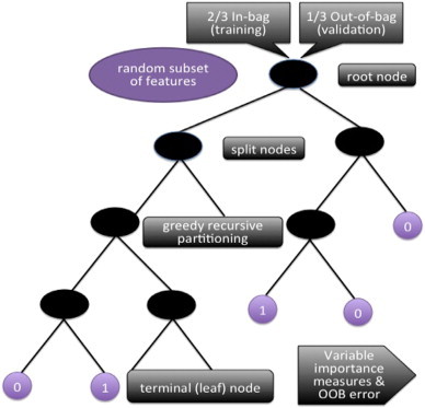
Random Forest procedure. For each classification tree (RF’s single unit), data are bootstrapped into in-bag and out-of-bag (for testing of the model). The tree starts with the in-bag data at the root node, with a random subset of features, and begins the process of “splitting.” The splitting criteria at each node are determined by a type of greedy algorithm that recursively partitions the data into daughter nodes, until reaching a terminal node. (Greedy recursive partitioning algorithms make the partitioning choice that performs best at each split, with the goal of globally optimal classification). The out-of-bag data are then sent down the tree as a test of model fit. The misclassification rate here is called “OOB error.” This is the internal validation process that prevents overfitting. Once all 10,000 trees in the forest have finished this process, the forest takes the majority vote from the trees, and obtains variable importance measures and OOB error.

In RF, the basic unit is a classification tree and the ensemble of trees (or forest) is used to classify participants using features (e.g., connectivity measures from fMRI; see Inline Supplementary Fig. S1). Each tree classifies or predicts a diagnostic status, and the forest's final prediction is the classification having the most votes based on all the trees in the forest. In random forests, it is not necessary to perform cross-validation or a separate test set to obtain an unbiased estimate of the test set error because validation is intrinsic to RF. Out-of-bag (OOB) error is estimated internally, during the RF run (http://www.stat.berkeley.edu/~breiman/RandomForests). Each tree in the forest is constructed using a bootstrap sample from the original data. The bootstrap randomly draws samples, with replacement from the original dataset. Each bootstrap sample will contain approximately two-thirds of the original observations, which results in one-third of the subjects being left out (i.e., not used in the construction of a particular tree). These out-of-bag samples are used to attain an unbiased estimate of the classification error (Breiman, 2001). The OOB error estimate can be shown to be almost identical to the error obtained by cross-validation (Hastie et al., 2009). RF is an example of bootstrap aggregation or bagging and is relatively protected from overfitting (Breiman, 2001). As an additional improvement of the bagging process, RF reduces the correlation between trees by using a subset of the variables at each split in the growing of each tree. RF also provides variable importance measures for feature selection. The OOB data are used to determine variable importance, based on mean decrease in accuracy. This is done for each tree by randomly permuting a variable in the OOB data and recording the change in accuracy or misclassification using the OOB data. For the ensemble of trees, the permuted predictions are aggregated and compared against the unpermuted predictions to determine the importance of the permuted variable by the magnitude of the decrease in accuracy of that variable. When the number of variables is very large (in the order of 2 × 10⁴), RF can be run once with all the variables, then again using only the most important variables selected from the first run.

Inline Supplementary Fig. S1 can be found online at http://dx.doi.org/10.1016/j.nicl.2015.04.002.

In the present study, we used the R package randomForest (Liaw and Wiener, 2002) for feature selection and classification analysis. As importance scores, proximity measures, and error rates vary because of the random components in RF (out of bag sampling, node-level permutation testing), we created a forest with a sufficient number of trees to ensure stability. To optimize the most important RF parameters, we fine-tuned the number of trees per forest to 10,000 as the plotted error rate was observed to stabilize (see Inline Supplementary Fig. S2), and set the number of variables randomly selected per node to 150, after tuning for this parameter. The RF algorithm ranked all features based on variable importance given by the mean decrease in accuracy. After the initial run with all features, we used the variable importance measures to select for 100 top informative features that were then used to build a classifier and obtain OOB error (see Inline Supplementary Fig. S3). Using these 100 features, we obtained the OOB error to assess how well the model predicted new data (see Inline Supplementary Fig. S4).

Inline Supplementary Figure S2.

Fig. S2.

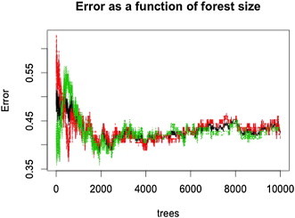
OOB error as a function of number of trees in the forest. Initially, the error fluctuates greatly, then eventually stabilizes with a large enough forest with 10,000 trees. Shown here are OOB errors using all 24,090 features prior to feature selection. The number of trees in the forest is an important parameter for fine-tuning to ensure stability of the algorithm. The red, green, and black lines represent the OOB errors for ASD, TD, and out-of-bag participants, respectively.

Inline Supplementary Figure S3.

Fig. S3.

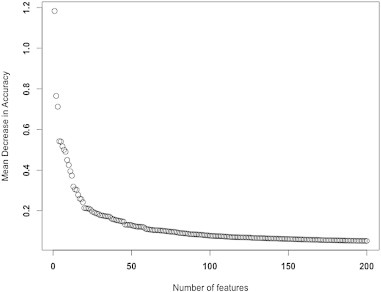
RF Feature selection using Mean Decrease Accuracy (MDA). In RF, variable importance is determined based on measures of mean decrease in accuracy. This is done for each tree by randomly permuting a variable in the OOB data and recording the change in accuracy. For the ensemble of trees, the permuted predictions are aggregated and compared against the unpermuted predictions to determine the importance of the permuted variable by the magnitude of the decrease in accuracy of that variable. We selected the top features using this MDA plot, where we observed stabilized rate of change of the MDA curve. Here, 100 features were selected using the MDA measures.

Inline Supplementary Figure S4.

Fig. S4.

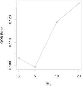
Fine tuning the mtry parameter for RF to select the optimal number of features to split at each node. Using the top 100 features, we fine tuned RF again on the parameter mtry, the number of features used at each split, to 5.

In the present study, we used the R package randomForest (Liaw and Wiener, 2002) for feature selection and classification analysis. As importance scores, proximity measures, and error rates vary because of the random components in RF (out of bag sampling, node-level permutation testing), we created a forest with a sufficient number of trees to ensure stability. To optimize the most important RF parameters, we fine-tuned the number of trees per forest to 10,000 as the plotted error rate was observed to stabilize (see Inline Supplementary Fig. S2), and set the number of variables randomly selected per node to 150, after tuning for this parameter. The RF algorithm ranked all features based on variable importance given by the mean decrease in accuracy. After the initial run with all features, we used the variable importance measures to select for 100 top informative features that were then used to build a classifier and obtain OOB error (see Inline Supplementary Fig. S3). Using these 100 features, we obtained the OOB error to assess how well the model predicted new data (see Inline Supplementary Fig. S4).

Inline Supplementary Figs. S2, S3, S4 can be found online at http://dx.doi.org/10.1016/j.nicl.2015.04.002.

3. Results

3.1. Classification accuracy of the three algorithms

The PSO-SVM achieved an accuracy of 81% on the training, and of 58% on the validation dataset, with 44% sensitivity and 72% specificity (for matching details, see Inline Supplementary Table S3). Accuracy for RFE-SVM was 100% on the training dataset and 66% on the validation dataset, with 60% sensitivity and 72% specificity. RF classified ASD with only 58% accuracy without feature selection. However, using the top 100 features with the highest variable importance (as defined above), RF achieved 90.8% accuracy (OOB error rate 9.2%), with sensitivity at 89% and specificity at 93%. In fact, using only the 10 most informative features, RF still attained an accuracy of 75%, with 75% sensitivity and 75% specificity. Note that the RF methodology does not have an external validation set, but the bootstrap sample of the data for each tree acts as an internal validation dataset. Using an external 20% validation set, accuracy from RF was at similar levels as for PSO and RFE (Inline Supplementary Table S4). However, since RF is an ensemble learning method, such external validation is not usually part of the RF procedure (see the Discussion section).

Inline Supplementary Table S3.

Table S3.

ABIDE cohort matching (p-values from independent two-sample t-tests).

	Full Sample	Training	Validation	Training <=> Validation	Training <=> Validation
	N = 252	N=200	N=52
	ASD <=> TD	ASD <=> TD	ASD <=> TD	ASD <=> ASD	TD <=> TD
Motion	0.923	0.922	0.984	0.985	0.984
Age	0.793	0.780	0.984	0.840	0.962
NVIQ	0.771	0.753	0.924	0.934	0.986
ADOS				0.824

Inline Supplementary Table S4.

Table S4.

Training and predictive (validation) accuracies for PSO-SVM, RFE-SVM, and RF, using external validation sets.

	PSO-SVM	RFE-SVM	RF
Training (N=200)	81%	100%	91%
Validation (N=52)	58%	66%	62%
Number of Features	100	40	150

The PSO-SVM achieved an accuracy of 81% on the training, and of 58% on the validation dataset, with 44% sensitivity and 72% specificity (for matching details, see Inline Supplementary Table S3). Accuracy for RFE-SVM was 100% on the training dataset and 66% on the validation dataset, with 60% sensitivity and 72% specificity. RF classified ASD with only 58% accuracy without feature selection. However, using the top 100 features with the highest variable importance (as defined above), RF achieved 90.8% accuracy (OOB error rate 9.2%), with sensitivity at 89% and specificity at 93%. In fact, using only the 10 most informative features, RF still attained an accuracy of 75%, with 75% sensitivity and 75% specificity. Note that the RF methodology does not have an external validation set, but the bootstrap sample of the data for each tree acts as an internal validation dataset. Using an external 20% validation set, accuracy from RF was at similar levels as for PSO and RFE (Inline Supplementary Table S4). However, since RF is an ensemble learning method, such external validation is not usually part of the RF procedure (see the Discussion section).

Inline Supplementary Tables S3, S4 can be found online at http://dx.doi.org/10.1016/j.nicl.2015.04.002.

3.2. Characterization of informative features from RF

Given the overall better performance from RF (compared to the other ML techniques), we proceeded to examine the most informative features selected by RF. When selecting only the 10 top features, several regions were noted to participate in two or more informative connections: left anterior cingulate gyrus, postcentral gyrus bilaterally, right precuneus, and left calcarine sulcus (see Inline Supplementary Fig. S5A). The pattern for the top 100 features, which yielded the peak accuracy of 91%, involved connections between 124 ROIs (see Inline Supplementary Fig. S5B). The left paracentral lobule and the right postcentral gyrus participated in ≥6 informative connections, which was ≥2SD above the mean participation among the 124 informative ROIs.

Inline Supplementary Figure S5.

Fig. S5.

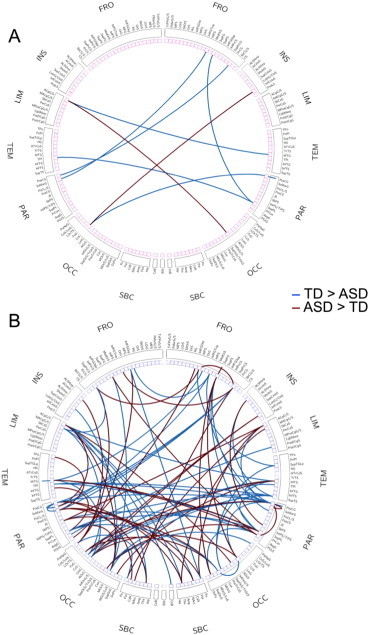
Connectogram showing informative connections. (A) Top 10 informative connections. (B) Top 100 informative connections. The labels of the connectograms can be found in Inline Supplementary Table S1, in the order in which they appear in the figure.

Given the overall better performance from RF (compared to the other ML techniques), we proceeded to examine the most informative features selected by RF. When selecting only the 10 top features, several regions were noted to participate in two or more informative connections: left anterior cingulate gyrus, postcentral gyrus bilaterally, right precuneus, and left calcarine sulcus (see Inline Supplementary Fig. S5A). The pattern for the top 100 features, which yielded the peak accuracy of 91%, involved connections between 124 ROIs (see Inline Supplementary Fig. S5B). The left paracentral lobule and the right postcentral gyrus participated in ≥6 informative connections, which was ≥2SD above the mean participation among the 124 informative ROIs.

Inline Supplementary Fig. S5 can be found online at http://dx.doi.org/10.1016/j.nicl.2015.04.002.

We further examined these top 100 features by functional networks, as defined in Power et al. (2011). We first determined the number of times ROIs from a specific network participated in an informative connection (Fig. 1A). The distribution differed significantly from the overall distribution of ROIs across different networks in Power et al. (χ² = 33.348, p = 0.001). Default mode, somatosensory/motor (hand region), and visual networks ranked at the top, accounting for half of all informative connections. We further examined normalized network importance (i.e., the number of times network ROIs participated in an informative connection divided by the total number of ROIs in the given network; Fig. 1B). This ratio highlighted the importance of somatosensory/motor networks (both mouth and hand regions), ahead of subcortical, memory retrieval, and visual networks. Within the two top networks, the somatosensory cortex (postcentral gyrus) participated in 23 of the top 100 connections, whereas the primary motor cortex (precentral gyrus) participated in only 9. Finally, we depicted the 100 top connections in a heat map matrix (Fig. 1C), which highlighted the importance of connections between DMN and visual ROIs (14 informative features). Informative features for the somatosensory/motor hand regions were dominated by connections with subcortical ROIs.

Fig. 1.

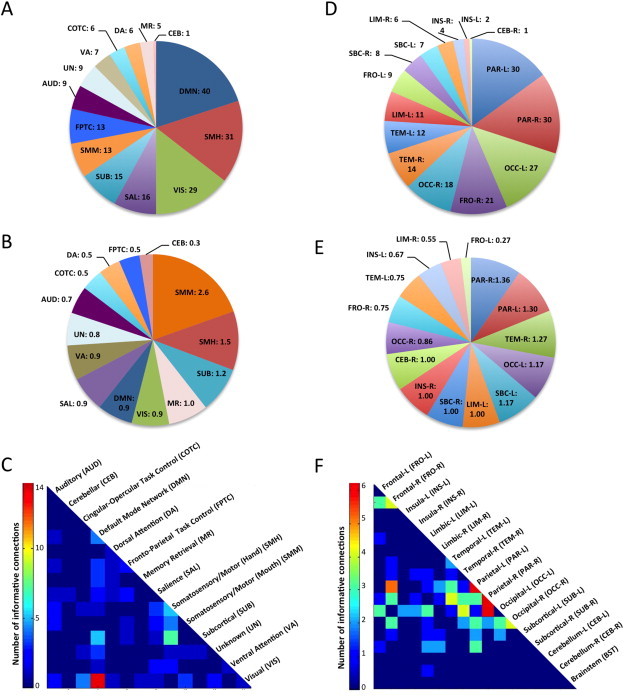
Informative features selected by RF. (A) Pie chart showing the number of informative ROIs per functional network. (B) Normalized number of informative ROIs per network (ratio of the number of times network ROIs participate in an informative connection divided by the total number of ROIs in given network). This number can exceed 1 because a given ROI may participate in several informative connections. (C) Heatmap of informative connections by functional networks. (D) Number of informative ROIs per anatomical parcellation. (E) Normalized number of informative ROIs per anatomical parcel (ratio of the number of times anatomical ROIs participate in an informative connection divided by the total number of ROIs in given parcel). (F) Heatmap of informative connections by anatomical parcel.

Examining the 100 top features by broad anatomical subdivisions (Fischl et al., 2004), the distribution did not differ significantly from expected (χ² = 5.225, p = 0.98). We found 60 participations by parietal lobes bilaterally, followed by 45 for occipital lobes bilaterally. The right frontal lobe also had heightened density of informative connections (with 21 participations; Fig. 1D). When normalizing participations by the number of ROIs within each subdivision (analogous to the procedure described above), the bilateral parietal lobes again stood out, followed by the right temporal lobe (Fig. 1E). On the heat map matrix (Fig. 1F), the highest concentration of the most informative connections was found to involve the parietal lobes bilaterally, with six informative connections each within the left and right parietal lobes, and an additional six between the right parietal and left occipital lobes and five between the left parietal and right frontal lobes.

We examined the 100 top features by several other criteria. They were almost evenly divided with respect to the direction of mean FC differences (45% over-, 55% underconnected in the ASD group) and type of connection (49% inter-, 51% intra-hemispheric). 95% of the top connections were between networks, 5% were within networks, 87% were mid- to long-distance (>40 mm Euclidean distance), and 11% were short-distance (<40 mm). However, these percentages of Euclidean distance (χ² = 0.228, p-value = 0.63) and of network connection (χ² = 2.24, p-value = 0.13) did not differ significantly from those expected based on the totality of 24,090 features examined in the entire connectivity matrix.

4. Discussion

In this study, we used intrinsic functional connectivities between a set of functionally defined ROIs (Power et al., 2011) for machine learning diagnostic classification of ASD. While accuracy remained overall modest for PSO-SVM and RFE-SVM approaches, it was high (91%) for random forest. The RF algorithm is well-suited for classification of fcMRI data for several reasons: It (i) is applicable when there are more features than observations, (ii) performs embedded feature selection and is relatively insensitive to any large number of irrelevant features, (iii) incorporates interactions between features, (iv) is based on the theory of ensemble learning that allows the algorithm to learn accurately both simple and complex classification functions, and (v) is applicable for both binary and multi-category classification tasks (Breiman, 2001).

4.1. Regions and networks

We examined in two steps which single regions and functional networks were most ‘informative’, contributing most heavily to diagnostic classification. First, focusing on only the ten top features, for which an accuracy of 75% was achieved, we found that limbic (left anterior cingulate), somatosensory (postcentral gyri bilaterally), visual (calcarine sulcus), and default mode (right precuneus) regions stood out (Supplementary Fig. 3A). This was largely supported by subsequent examination of the 100 top features, for which the peak classification accuracy of 91% was reached. Half of all ROIs involved in these connections belonged to three (out of 14) networks, which were default mode, somatosensory/motor (hand) and visual (Fig. 1A).

The informative role of the DMN in diagnostic classification was not surprising, given extensive evidence of DMN anomalies in ASD. These include fMRI findings indicating failure to enter the default mode in ASD (Kennedy et al., 2006; Murdaugh et al., 2012), as well as numerous fcMRI reports of atypical connectivity of the DMN (Assaf et al., 2010; Courchesne et al., 2005; Di Martino et al., 2013; Keown et al., 2013; Monk et al., 2009; Redcay et al., 2013; Uddin et al., 2013b; von dem Hagen et al., 2013; Washington et al., 2014; Zielinski et al., 2012). Functionally, the DMN is considered to relate to self-referential cognition, including domains of known impairment in ASD, such as theory of mind and affective decision making (Andrews-Hanna et al., 2010).

The visual system appears to be overall relatively spared in ASD (Simmons et al., 2009), and atypically enhanced participation of the visual cortex has been observed across many fMRI (Samson et al., 2012) and fcMRI studies (Shen et al., 2012), with the added recent finding of atypically increased local functional connectivity in ASD being associated with symptom severity (Keown et al., 2013). The relative importance of visual regions and occipital lobes probably reflects atypical function of the visual system in ASD (Dakin and Frith, 2005) rather than integrity.

The role of somatosensory regions was particularly prominent when considering a normalized ratio of informative ROIs (Fig. 1B). Although only a total of 26 somatosensory/motor ROIs (hand and mouth regions combined) were included in the analysis, these participated in 44 out of the 100 most informative connections. This effect was distinctly driven by the primary somatosensory cortex in the postcentral gyrus (rather than motor cortex). Our finding may be related to impaired emotional recognition of facial expressions in patients with focal damage to the right somatosensory cortices (SI and SII) observed by Adolphs and colleagues (2000), given that perception of facial expressions is also frequently impaired in individuals with ASD (Nuske et al., 2013). Although somatosensory anomalies have been described in a number of ASD studies (Puts et al., 2014; Tomchek and Dunn, 2007; Tommerdahl et al., 2007), the highly prominent role of somatosensory regions in diagnostic classification was remarkable. The imaging literature on the somatosensory cortex in ASD is currently limited. Cascio and colleagues (2012) found atypical activation patterns in adults with ASD for pleasant and unpleasant tactile stimuli in the PCC and insula, which could reflect altered functional connectivity with the somatosensory cortex (not tested in the cited study). Atypical postcentral responses to somatosensory stimuli have also been observed in one evoked potential study in young children with ASD (Miyazaki et al., 2007). Although little is known about differential responses between ASD and TD groups to resting state instructions or confined conditions within bore and head coil during scanning, it is possible that tactile or proprioceptive processing had some effect on the role of somatosensory ROIs in diagnostic classification. However, focus on low frequencies in our study would be expected to emphasize intrinsic fluctuations (thought to reflect history of co-activation (Lewis et al., 2009)) over online processing effects that tend to occur at higher frequencies.

4.2. Issues, caveats, and perspectives

Diagnostic classification accuracy achieved using random forest machine learning was distinctly above accuracies reported from previous studies using rs-fcMRI (Anderson et al., 2011), including a recent publication (Nielsen et al., 2013) using the same consortium database as in the present study. This was likely due to its advantages as an ensemble learning method. RF implements a bootstrapping ‘out-of-bag’ validation process (randomly selected subsamples), contrary to the other machine learning tools (PSO-SVM, RFE-SVM) used here, which required external validation datasets. This latter procedure may provide stringent protection from overfitting to the idiosyncrasies of any given training dataset, as may be seen with conventional leave-one-out validation (Ecker et al., 2010a; Ecker et al., 2010b; Iidaka, 2015; Ingalhalikar et al., 2011; Nielsen et al., 2013). The procedure depends, however, on the assumption that training and validation samples can be adequately matched. Such matching may be difficult, if many variables (e.g., age, sex, motion, site, eye status, scanner, imaging protocol) are potentially relevant (cf. Online Supplementary Table A.1). Aggravating the problem, some potentially crucial variables, such as IQ, symptom severity, and handedness, were incomplete in ABIDE (missing for some sites) and could thus not be well matched. Other possibly important variables, some of which are hard to operationalize (e.g., history of interventions, medication) were entirely unavailable. Even if matching on all those variables were possible, a more intractable problem would remain. There is general consensus that ASD is an umbrella term for several – maybe many – underlying biological subtypes (Jeste and Geschwind, 2014), which are currently unknown. Any substantial difference between training and validation datasets in the composition of these subtypes, which cannot be detected and cannot therefore be avoided, is likely to result in poor prediction in a validation dataset. In ASD machine learning classification, accuracy will tend to be overestimated in training datasets (with common leave-one-out procedure), but underestimated in external validation datasets because of the problems described above. Indeed, when using such a split into training and external validation sets, RF yielded accuracies similar to PSO and RFE-SVM. However, such split is inconsistent with RF as an ensemble learning technique, which instead implements out-of-bag validation. In our view, this approach presents a solution to the matching problems described above, as the bootstrapping procedure itself ensures matching of training and validation datasets. This solution may be considered ideal, given the currently available sample limitations even from consortium datasets. As described in Section 2.2, the mandatory (Power et al., 2015; Satterthwaite et al., 2013) selection of low-motion data reduced the initially large ABIDE sample to only 252 participants. External 20% validation sets included only 26 participants per group, highlighting the matching issues described above. Distinctly larger high-quality datasets may in the future allow investigators to go beyond the pragmatic bootstrapping solution offered by RF and return to even more stringent external validation procedures because the probability of adequate matching for unknown subtypes by chance alone will increase with much larger numbers.

Our findings suggest that intrinsic functional connectivity may identify complex biomarkers of ASD, which is not unexpected given the extensive literature on functional connectivity anomalies in this disorder (e.g., Vissers et al., 2012). Aside from the use of RF machine learning and its virtues described above, the main difference between our study and the relatively unsuccessful classification study by Nielsen et al. (2013) was our careful selection of high-quality (low-motion) datasets, resulting in the inclusion of only 252 (out of a total of 1112) participants, equally divided between two tightly motion-matched diagnostic groups. Our procedure was informed by the recent flurry of studies suggesting that even small amounts of head motion well below 1 mm affect interregional fMRI signal correlations (Carp, 2011; Jo et al., 2013; Power et al., 2013b; Power et al., 2014; Satterthwaite et al., 2013; Van Dijk et al., 2012).

Although we modeled effects of site, the use of multisite data with the numerous factors of variability it entails remains a challenge that needs to be accepted as high-quality rs-fMRI data for comparable sample sizes from a single site are not currently available. Inclusion of 126 ASD participants may provide relative protection from cohort effects that are probably at work in many small-sample imaging studies. However, the need for high levels of compliance in fMRI studies, even when there is no explicit task, inevitably results in inclusionary biases because low-functioning people with ASD are unable to participate. The methodologically indispensable step of selecting low-motion data probably added to this issue, given that higher-functioning participants were likely to move less during scanning. Indeed, our diagnostic groups were matched for nonverbal IQ, and relatively few ASD participants with intellectual disability and IQs below 70 were included. The pattern of informative connections observed in our study may therefore not apply to the lower-functioning end of the autism spectrum.

A high diagnostic classification accuracy was reached for the 100 most informative features. The pattern of these connections was highly complex, involving numerous brain regions. While some networks (somatosensory, default mode, visual) stood out, many others contributed to the classification. This may be disappointing to anyone harboring the hope that the neurobiology of ASD might ultimately be pinned down to simple and localizable causes. However, the literature on functional and anatomical brain anomalies in ASD is fully consistent with the concept of a disorder with highly distributed, rather than localized, patterns (Akshoomoff et al., 2002; Müller, 2007; Philip et al., 2012; Vissers et al., 2012; Wass, 2011). The complex pattern (cf. Supplementary Fig. 5B) should, however, not be viewed as definitive for the ASD population as a whole (in particular lower-functioning segments). Instead, it reflects a distinctive connectivity pattern for a large cohort of children and young adults with ASD. Sample size, careful data denoising, and refinement of machine learning approaches in the present study thus present a distinct advance in the search for functional connectivity biomarkers of ASD, but given the challenges described above, much further work remains to be done. Although fcMRI is generally accepted as a powerful technique for identifying network abnormalities, the addition of complementary techniques (e.g., diffusion weighted MRI for assays of anatomical connectivity; magnetoencephalography for detection of neuronal coherence in high-frequency bands) will likely enhance diagnostic classification and the detection of complex biomarkers (see Zhou et al. (2014) for a recent multimodal attempt with moderate success). However, it is also important to recognize that machine learning diagnostic classification can only be performed at the level permitted by the diagnostic procedure itself, which is fundamentally imperfect. It cannot be expected that a disorder recognized as neurobiological in nature would be detected by means of purely behavioral and observational criteria currently used for diagnosis. There can thus be no perfect fit between brain markers and diagnostic labels. The contribution of machine learning to the discovery of biomarkers, which can ultimately replace behavioral criteria, is therefore important.

Appendix A. Supplementary data

Supplementary material.

References

- Adolphs R., Damasio H., Tranel D., Cooper G., Damasio A.R. A role for somatosensory cortices in the visual recognition of emotion as revealed by three-dimensional lesion mapping. J. Neurosci. 2000;20(7):2683–2690. doi: 10.1523/JNEUROSCI.20-07-02683.2000. 10729349 [DOI] [PMC free article] [PubMed] [Google Scholar]
- Akshoomoff N., Pierce K., Courchesne E. The neurobiological basis of autism from a developmental perspective. Dev. Psychopathol. 2002;14(3):613–634. doi: 10.1017/s0954579402003115. 12349876 [DOI] [PubMed] [Google Scholar]
- American Psychiatric Association . Diagnostic and Statistical Manual of Mental Disorders — V. fourth edition. American Psychiatric Association; Washington, DC: 2013. [Google Scholar]
- Anderson J.S., Nielsen J.A., Froehlich A.L., DuBray M.B., Druzgal T.J., Cariello A.N., Cooperrider J.R., Zielinski B.A., Ravichandran C., Fletcher P.T., Alexander A.L., Bigler E.D., Lange N., Lainhart J.E. Functional connectivity magnetic resonance imaging classification of autism. Brain. 2011;134(12):3742–3754. doi: 10.1093/brain/awr263. 22006979 [DOI] [PMC free article] [PubMed] [Google Scholar]
- Andrews-Hanna J.R., Reidler J.S., Sepulcre J., Poulin R., Buckner R.L. Functional–anatomic fractionation of the brain's default network. Neuron. 2010;65(4):550–562. doi: 10.1016/j.neuron.2010.02.005. 20188659 [DOI] [PMC free article] [PubMed] [Google Scholar]
- Assaf M., Jagannathan K., Calhoun V.D., Miller L., Stevens M.C., Sahl R., O'Boyle J.G., Schultz R.T., Pearlson G.D. Abnormal functional connectivity of default mode sub-networks in autism spectrum disorder patients. Neuroimage. 2010;53(1):247–256. doi: 10.1016/j.neuroimage.2010.05.067. 20621638 [DOI] [PMC free article] [PubMed] [Google Scholar]
- Breiman L. Random Forests. Machine Learning. 2001;45:5–32. [Google Scholar]
- Carp J. Optimizing the order of operations for movement scrubbing: comment on Power et al. Neuroimage. 2013;76:436–438. doi: 10.1016/j.neuroimage.2011.12.061. 22227884 [DOI] [PubMed] [Google Scholar]
- Carp J. Optimizing the order of operations for movement scrubbing: comment on Power et al. Neuroimage. 2011 doi: 10.1016/j.neuroimage.2011.12.061. [DOI] [PubMed] [Google Scholar]
- Cascio C.J., Moana-Filho E.J., Guest S., Nebel M.B., Weisner J., Baranek G.T., Essick G.K. Perceptual and neural response to affective tactile texture stimulation in adults with autism spectrum disorders. Autism Res. 2012;5(4):231–244. doi: 10.1002/aur.1224. 22447729 [DOI] [PMC free article] [PubMed] [Google Scholar]
- Cordes D., Haughton V.M., Arfanakis K., Carew J.D., Turski P.A., Moritz C.H., Quigley M.A., Meyerand M.E. Frequencies contributing to functional connectivity in the cerebral cortex in “resting-state” data. A.J.N.R. Am. J. Neuroradiol. 2001;22(7):1326–1333. 11498421 [PMC free article] [PubMed] [Google Scholar]
- Courchesne E., Redcay E., Morgan J.T., Kennedy D.P. Autism at the beginning: microstructural and growth abnormalities underlying the cognitive and behavioral phenotype of autism. Dev. Psychopathol. 2005;17(3):577–597. doi: 10.1017/S0954579405050285. 16262983 [DOI] [PubMed] [Google Scholar]
- Cox R.W. AFNI: software for analysis and visualization of functional magnetic resonance neuroimages. Comput. Biomed. Res. 1996;29(3):162–173. doi: 10.1006/cbmr.1996.0014. 8812068 [DOI] [PubMed] [Google Scholar]
- Dakin S., Frith U. Vagaries of visual perception in autism. Neuron. 2005;48(3):497–507. doi: 10.1016/j.neuron.2005.10.018. 16269366 [DOI] [PubMed] [Google Scholar]
- Di Martino A., Yan C.G., Li Q., Denio E., Castellanos F.X., Alaerts K., Anderson J.S., Assaf M., Bookheimer S.Y., Dapretto M., Deen B., Delmonte S., Dinstein I., Ertl-Wagner B., Fair D.A., Gallagher L., Kennedy D.P., Keown C.L., Keysers C., Lainhart J.E., Lord C., Luna B., Menon V., Minshew N.J., Monk C.S., Mueller S., Müller R.A., Nebel M.B., Nigg J.T., O’Hearn K., Pelphrey K.A., Peltier S.J., Rudie J.D., Sunaert S., Thioux M., Tyszka J.M., Uddin L.Q., Verhoeven J.S., Wenderoth N., Wiggins J.L., Mostofsky S.H., Milham M.P. The autism brain imaging data exchange: towards a large-scale evaluation of the intrinsic brain architecture in autism. Mol. Psychiatry. 2014;19(6):659–667. doi: 10.1038/mp.2013.78. 23774715 [DOI] [PMC free article] [PubMed] [Google Scholar]
- Di Martino A., Zuo X.N., Kelly C., Grzadzinski R., Mennes M., Schvarcz A., Rodman J., Lord C., Castellanos F.X., Milham M.P. Shared and distinct intrinsic functional network centrality in autism and attention-deficit/hyperactivity disorder. Biol. Psychiatry. 2013;74:623–632. doi: 10.1016/j.biopsych.2013.02.011. 23541632 [DOI] [PMC free article] [PubMed] [Google Scholar]
- Ecker C., Marquand A., Mourão-Miranda J., Johnston P., Daly E.M., Brammer M.J., Maltezos S., Murphy C.M., Robertson D., Williams S.C., Murphy D.G. Describing the brain in autism in five dimensions — magnetic resonance imaging-assisted diagnosis of autism spectrum disorder using a multiparameter classification approach. J. Neurosci. 2010;30(32):10612–10623. doi: 10.1523/JNEUROSCI.5413-09.2010. 20702694 [DOI] [PMC free article] [PubMed] [Google Scholar]
- Ecker C., Rocha-Rego V., Johnston P., Mourao-Miranda J., Marquand A., Daly E.M., Brammer M.J., Murphy C., Murphy D.G., MRC AIMS Consortium Investigating the predictive value of whole-brain structural MR scans in autism: a pattern classification approach. Neuroimage. 2010;49(1):44–56. doi: 10.1016/j.neuroimage.2009.08.024. 19683584 [DOI] [PubMed] [Google Scholar]
- Fischl B., van der Kouwe A., Destrieux C., Halgren E., Ségonne F., Salat D.H., Busa E., Seidman L.J., Goldstein J., Kennedy D., Caviness V., Makris N., Rosen B., Dale A.M. Automatically parcellating the human cerebral cortex. Cereb. Cortex. 2004;14(1):11–22. doi: 10.1093/cercor/bhg087. 14654453 [DOI] [PubMed] [Google Scholar]
- Geschwind D.H., Levitt P. Autism spectrum disorders: developmental disconnection syndromes. Curr. Opin. Neurobiol. 2007;17(1):103–111. doi: 10.1016/j.conb.2007.01.009. 17275283 [DOI] [PubMed] [Google Scholar]
- Guyon I., Weston J., Barnhill S., Vapnik V. Gene selection for cancer classification using support vector machines. Mach. Learn. 2002;46(1/3):389–422. [Google Scholar]
- Hastie T., Tibshirani R., Friedman J. The Elements of Statistical Learning: Data Mining Inference and Prediction. Springer; 2009. [Google Scholar]
- Iidaka T. Resting state functional magnetic resonance imaging and neural network classified autism and control. Cortex. 2015;63:55–67. doi: 10.1016/j.cortex.2014.08.011. 25243989 [DOI] [PubMed] [Google Scholar]
- Ingalhalikar M., Parker D., Bloy L., Roberts T.P., Verma R. Diffusion based abnormality markers of pathology: toward learned diagnostic prediction of ASD. Neuroimage. 2011;57(3):918–927. doi: 10.1016/j.neuroimage.2011.05.023. 21609768 [DOI] [PMC free article] [PubMed] [Google Scholar]
- Irimia A., Chambers M.C., Torgerson C.M., Van Horn J.D. Circular representation of human cortical networks for subject and population-level connectomic visualization. Neuroimage. 2012;60(2):1340–1351. doi: 10.1016/j.neuroimage.2012.01.107. 22305988 [DOI] [PMC free article] [PubMed] [Google Scholar]
- Jeste S.S., Geschwind D.H. Disentangling the heterogeneity of autism spectrum disorder through genetic findings. Nat. Rev. Neurol. 2014;10(2):74–81. doi: 10.1038/nrneurol.2013.278. 24468882 [DOI] [PMC free article] [PubMed] [Google Scholar]
- Jo H.J., Gotts S.J., Reynolds R.C., Bandettini P.A., Martin A., Cox R.W., Saad Z.S. Effective preprocessing procedures virtually eliminate distance-dependent motion artifacts in resting state FMRI. J. Appl. Math. 2013;2013:2013. doi: 10.1155/2013/935154. 24415902 [DOI] [PMC free article] [PubMed] [Google Scholar]
- Kennedy D.P., Redcay E., Courchesne E. Failing to deactivate: resting functional abnormalities in autism. Proc. Natl. Acad. Sci. U. S. A. 2006;103(21):8275–8280. doi: 10.1073/pnas.0600674103. 16702548 [DOI] [PMC free article] [PubMed] [Google Scholar]
- Kennedy J., Eberhart R. Particle swarm optimization. Neural Netw. 1995;4:1942–1948. [Google Scholar]
- Keown C.L., Shih P., Nair A., Peterson N., Mulvey M.E., Müller R.A. Local functional overconnectivity in posterior brain regions is associated with symptom severity in autism spectrum disorders. Cell Rep. 2013;5(3):567–572. doi: 10.1016/j.celrep.2013.10.003. 24210815 [DOI] [PMC free article] [PubMed] [Google Scholar]
- Lewis C.M., Baldassarre A., Committeri G., Romani G.L., Corbetta M. Learning sculpts the spontaneous activity of the resting human brain. Proc. Natl. Acad. Sci. U. S. A. 2009;106(41):17558–17563. doi: 10.1073/pnas.0902455106. 19805061 [DOI] [PMC free article] [PubMed] [Google Scholar]
- Liaw A., Wiener M. Classification and regression by random forest. R News. 2002;2:18–22. [Google Scholar]
- Miyazaki M., Fujii E., Saijo T., Mori K., Hashimoto T., Kagami S., Kuroda Y. Short-latency somatosensory evoked potentials in infantile autism: evidence of hyperactivity in the right primary somatosensory area. Dev. Med. Child Neurol. 2007;49(1):13–17. doi: 10.1017/s0012162207000059.x. 17209970 [DOI] [PubMed] [Google Scholar]
- Monk C.S., Peltier S.J., Wiggins J.L., Weng S.J., Carrasco M., Risi S., Lord C. Abnormalities of intrinsic functional connectivity in autism spectrum disorders. Neuroimage. 2009;47(2):764–772. doi: 10.1016/j.neuroimage.2009.04.069. 19409498 [DOI] [PMC free article] [PubMed] [Google Scholar]
- Müller R.-A. The study of autism as a distributed disorder. Ment. Retard. Dev. Disabil. Res. Rev. 2007;13(1):85–95. doi: 10.1002/mrdd.20141. 17326118 [DOI] [PMC free article] [PubMed] [Google Scholar]
- Müller R.-A., Shih P., Keehn B., Deyoe J.R., Leyden K.M., Shukla D.K. Underconnected, but how? A survey of functional connectivity MRI studies in autism spectrum disorders. Cereb. Cortex. 2011;21(10):2233–2243. doi: 10.1093/cercor/bhq296. 21378114 [DOI] [PMC free article] [PubMed] [Google Scholar]
- Murdaugh D.L., Shinkareva S.V., Deshpande H.R., Wang J., Pennick M.R., Kana R.K. Differential deactivation during mentalizing and classification of autism based on default mode network connectivity. PLOS One. 2012;7(11):e50064. doi: 10.1371/journal.pone.0050064. 23185536 [DOI] [PMC free article] [PubMed] [Google Scholar]
- Nair A., Keown C.L., Datko M., Shih P., Keehn B., Müller R.A. Impact of methodological variables on functional connectivity findings in autism spectrum disorders. Hum. Brain Mapp. 2014;35(8):4035–4048. doi: 10.1002/hbm.22456. 24452854 [DOI] [PMC free article] [PubMed] [Google Scholar]
- Nielsen J.A., Zielinski B.A., Fletcher P.T., Alexander A.L., Lange N., Bigler E.D., Lainhart J.E., Anderson J.S. Multisite functional connectivity MRI classification of autism: ABIDE results. Front. Hum. Neurosci. 2013;7:599. doi: 10.3389/fnhum.2013.00599. 24093016 [DOI] [PMC free article] [PubMed] [Google Scholar]
- Nuske H.J., Vivanti G., Dissanayake C. Are emotion impairments unique to, universal, or specific in autism spectrum disorder? A comprehensive review. Cognition & Emotion. 2013;27(6):1042–1061. doi: 10.1080/02699931.2012.762900. [DOI] [PubMed] [Google Scholar]
- Philip R.C., Dauvermann M.R., Whalley H.C., Baynham K., Lawrie S.M., Stanfield A.C. A systematic review and meta-analysis of the fMRI investigation of autism spectrum disorders. Neurosci. Biobehav. Rev. 2012;36(2):901–942. doi: 10.1016/j.neubiorev.2011.10.008. 22101112 [DOI] [PubMed] [Google Scholar]
- Power J.D., Barnes K.A., Snyder A.Z., Schlaggar B.L., Petersen S.E. Spurious but systematic correlations in functional connectivity MRI networks arise from subject motion. Neuroimage. 2012;59(3):2142–2154. doi: 10.1016/j.neuroimage.2011.10.018. 22019881 [DOI] [PMC free article] [PubMed] [Google Scholar]
- Power J.D., Barnes K.A., Snyder A.Z., Schlaggar B.L., Petersen S.E. Steps toward optimizing motion artifact removal in functional connectivity MRI; a reply to Carp. Neuroimage. 2013;76:439–441. doi: 10.1016/j.neuroimage.2012.03.017. 22440651 [DOI] [PMC free article] [PubMed] [Google Scholar]
- Power J.D., Cohen A.L., Nelson S.M., Wig G.S., Barnes K.A., Church J.A., Vogel A.C., Laumann T.O., Miezin F.M., Schlaggar B.L., Petersen S.E. Functional network organization of the human brain. Neuron. 2011;72(4):665–678. doi: 10.1016/j.neuron.2011.09.006. 22099467 [DOI] [PMC free article] [PubMed] [Google Scholar]
- Power J.D., Mitra A., Laumann T.O., Snyder A.Z., Schlaggar B.L., Petersen S.E. Methods to detect, characterize, and remove motion artifact in resting state fMRI. Neuroimage. 2014;84:320–341. doi: 10.1016/j.neuroimage.2013.08.048. 23994314 [DOI] [PMC free article] [PubMed] [Google Scholar]
- Power J.D., Schlaggar B.L., Petersen S.E. Recent progress and outstanding issues in motion correction in resting state fMRI. Neuroimage. 2015;105:536–551. doi: 10.1016/j.neuroimage.2014.10.044. 25462692 [DOI] [PMC free article] [PubMed] [Google Scholar]
- Puts N.A., Wodka E.L., Tommerdahl M., Mostofsky S.H., Edden R.A. Impaired tactile processing in children with autism spectrum disorder. J. Neurophysiol. 2014;111(9):1803–1811. doi: 10.1152/jn.00890.2013. 24523518 [DOI] [PMC free article] [PubMed] [Google Scholar]
- Redcay E., Moran J.M., Mavros P.L., Tager-Flusberg H., Gabrieli J.D., Whitfield-Gabrieli S. Intrinsic functional network organization in high-functioning adolescents with autism spectrum disorder. Front. Hum. Neurosci. 2013;7:573. doi: 10.3389/fnhum.2013.00573. 24062673 [DOI] [PMC free article] [PubMed] [Google Scholar]
- Samson F., Mottron L., Soulières I., Zeffiro T.A. Enhanced visual functioning in autism: an ALE meta-analysis. Hum. Brain Mapp. 2012;33(7):1553–1581. doi: 10.1002/hbm.21307. 21465627 [DOI] [PMC free article] [PubMed] [Google Scholar]
- Satterthwaite T.D., Elliott M.A., Gerraty R.T., Ruparel K., Loughead J., Calkins M.E., Eickhoff S.B., Hakonarson H., Gur R.C., Gur R.E., Wolf D.H. An improved framework for confound regression and filtering for control of motion artifact in the preprocessing of resting-state functional connectivity data. Neuroimage. 2013;64:240–256. doi: 10.1016/j.neuroimage.2012.08.052. 22926292 [DOI] [PMC free article] [PubMed] [Google Scholar]
- Schipul S.E., Keller T.A., Just M.A. Inter-regional brain communication and its disturbance in autism. Front. Syst. Neurosci. 2011;5:10. doi: 10.3389/fnsys.2011.00010. 21390284 [DOI] [PMC free article] [PubMed] [Google Scholar]
- Shen M.D., Shih P., Öttl B., Keehn B., Leyden K.M., Gaffrey M.S., Müller R.A. Atypical lexicosemantic function of extrastriate cortex in autism spectrum disorder: evidence from functional and effective connectivity. Neuroimage. 2012;62(3):1780–1791. doi: 10.1016/j.neuroimage.2012.06.008. 22699044 [DOI] [PMC free article] [PubMed] [Google Scholar]
- Simmons D.R., Robertson A.E., McKay L.S., Toal E., McAleer P., Pollick F.E. Vision in autism spectrum disorders. Vision Res. 2009;49(22):2705–2739. doi: 10.1016/j.visres.2009.08.005. 19682485 [DOI] [PubMed] [Google Scholar]
- Smith S.M., Jenkinson M., Woolrich M.W., Beckmann C.F., Behrens T.E., Johansen-Berg H., Bannister P.R., De Luca M., Drobnjak I., Flitney D.E., Niazy R.K., Saunders J., Vickers J., Zhang Y., De Stefano N., Brady J.M., Matthews P.M. Advances in functional and structural MR image analysis and implementation as FSL. Neuroimage. 2004;23(Suppl. 1):S208–S219. doi: 10.1016/j.neuroimage.2004.07.051. 15501092 [DOI] [PubMed] [Google Scholar]
- Tomchek S.D., Dunn W. Sensory processing in children with and without autism: a comparative study using the short sensory profile. Am. J. Occup. Ther. 2007;61(2):190–200. doi: 10.5014/ajot.61.2.190. 17436841 [DOI] [PubMed] [Google Scholar]
- Tommerdahl M., Tannan V., Cascio C.J., Baranek G.T., Whitsel B.L. Vibrotactile adaptation fails to enhance spatial localization in adults with autism. Brain Res. 2007;1154:116–123. doi: 10.1016/j.brainres.2007.04.032. 17498672 [DOI] [PMC free article] [PubMed] [Google Scholar]
- Uddin L.Q., Supekar K., Lynch C.J., Khouzam A., Phillips J., Feinstein C., Ryali S., Menon V. Salience network-based classification and prediction of symptom severity in children with autism. J.A.M.A. Psychiatry. 2013;70:869–879. doi: 10.1001/jamapsychiatry.2013.104. 23803651 [DOI] [PMC free article] [PubMed] [Google Scholar]
- Uddin L.Q., Supekar K., Menon V. Reconceptualizing functional brain connectivity in autism from a developmental perspective. Front. Hum. Neurosci. 2013;7:458. doi: 10.3389/fnhum.2013.00458. 23966925 [DOI] [PMC free article] [PubMed] [Google Scholar]
- Van Dijk K.R., Hedden T., Venkataraman A., Evans K.C., Lazar S.W., Buckner R.L. Intrinsic functional connectivity as a tool for human connectomics: theory, properties, and optimization. J. Neurophysiol. 2010;103(1):297–321. doi: 10.1152/jn.00783.2009. 19889849 [DOI] [PMC free article] [PubMed] [Google Scholar]
- Van Dijk K.R., Sabuncu M.R., Buckner R.L. The influence of head motion on intrinsic functional connectivity MRI. Neuroimage. 2012;59(1):431–438. doi: 10.1016/j.neuroimage.2011.07.044. 21810475 [DOI] [PMC free article] [PubMed] [Google Scholar]
- Vissers M.E., Cohen M.X., Geurts H.M. Brain connectivity and high functioning autism: a promising path of research that needs refined models, methodological convergence, and stronger behavioral links. Neurosci. Biobehav. Rev. 2012;36(1):604–625. doi: 10.1016/j.neubiorev.2011.09.003. 21963441 [DOI] [PubMed] [Google Scholar]
- Von dem Hagen E.A., Stoyanova R.S., Baron-Cohen S., Calder A.J. Reduced functional connectivity within and between ‘social’ resting state networks in autism spectrum conditions. Soc. Cogn. Affect. Neurosci. 2013;8:694–701. doi: 10.1093/scan/nss053. 22563003 [DOI] [PMC free article] [PubMed] [Google Scholar]
- Washington S.D., Gordon E.M., Brar J., Warburton S., Sawyer A.T., Wolfe A., Mease-Ference E.R., Girton L., Hailu A., Mbwana J., Gaillard W.D., Kalbfleisch M.L., Vanmeter J.W. Dysmaturation of the default mode network in autism. Hum. Brain Mapp. 2014;35:1284–1296. doi: 10.1002/hbm.22252. 23334984 [DOI] [PMC free article] [PubMed] [Google Scholar]
- Wass S. Distortions and disconnections: disrupted brain connectivity in autism. Brain Cogn. 2011;75(1):18–28. doi: 10.1016/j.bandc.2010.10.005. 21055864 [DOI] [PubMed] [Google Scholar]
- Zhang Y., Brady M., Smith S. Segmentation of brain MR images through a hidden Markov random field model and the expectation–maximization algorithm. I. E.E.E. Transactions Med. Imaging. 2001;20(1):45–57. doi: 10.1109/42.906424. 11293691 [DOI] [PubMed] [Google Scholar]
- Zhou Y., Yu F., Duong T. Multiparametric MRI characterization and prediction in autism spectrum disorder using graph theory and machine learning. PLOS One. 2014;9(6):e90405. doi: 10.1371/journal.pone.0090405. 24922325 [DOI] [PMC free article] [PubMed] [Google Scholar]
- Zielinski B.A., Anderson J.S., Froehlich A.L., Prigge M.B., Nielsen J.A., Cooperrider J.R., Cariello A.N., Fletcher P.T., Alexander A.L., Lange N., Bigler E.D., Lainhart J.E. scMRI reveals large-scale brain network abnormalities in autism. PLOS One. 2012;7(11):e49172. doi: 10.1371/journal.pone.0049172. 23185305 [DOI] [PMC free article] [PubMed] [Google Scholar]
Associated Data
This section collects any data citations, data availability statements, or supplementary materials included in this article.
Supplementary Materials