

Abstract
Similar activity patterns at both neuron and network levels can arise from different combinations of membrane and synaptic conductance values. A strategy by which neurons may preserve their electrical output is via cell type-dependent balances of inward and outward currents. Measurements of mRNA transcripts that encode ion channel proteins within motor neurons in the crustacean cardiac ganglion recently revealed correlations between certain channel types. To determine whether balances of intrinsic currents potentially resulting from such correlations preserve certain electrical cell outputs, we developed a nominal biophysical model of the crustacean cardiac ganglion using biological data. Predictions from the nominal model showed that coregulation of ionic currents may preserve the key characteristics of motor neuron activity. We then developed a methodology of sampling a multidimensional parameter space to select an appropriate model set for meaningful comparison with variations in correlations seen in biological datasets.
Introduction
Neurons of the same cell type may be expected to have identical intrinsic membrane properties, both within an animal and across individuals. Yet recent work has argued that similar activity patterns, both at single neuron and network levels, can arise from variable levels and combinations of membrane and synaptic conductance levels (Prinz et al., 2004; Swensen and Bean, 2005; Achard and De Schutter, 2006; Marder and Goaillard, 2006; Schulz et al., 2006; Tobin and Calabrese, 2006; Marder et al., 2007; Taylor et al., 2009). Similarly, such variability also exists in levels of mRNAs that encode for channels that carry ionic currents (Schulz et al., 2006, 2007). However, these examples of variability are constrained in that different sets of ionic conductances (Khorkova and Golowasch, 2007) and ion channel mRNA levels (Schulz et al., 2007; Tobin et al., 2009) are strongly correlated with one another in different classes of identified neurons. These results suggest that cellular output in the nervous system may not be of a fixed, developmental origin, but rather be determined in part by an ongoing regulation of characteristic sets of correlated or coregulated ionic conductances and/or channels. Such an understanding of basic neuronal function has a profound impact on our understanding of nervous system function in general, from cellular, network, and behavioral perspectives.
Computational models have been used to explore the parameter space to determine how groups of conductances both alter and preserve neuronal output. Prinz et al. (2003) explored the maximal conductance space of a single-compartment model neuron to quantify the numerous types of spiking and bursting models that emerged. This database of resulting model neurons was used to demonstrate that similar patterns of activity could be produced by many different parameter sets, both for single neurons (Prinz et al., 2003) and within small networks (Prinz et al., 2004). Such a model-based parameter space exploration also has been used to explore the effects of varying conductance densities on output patterns for a globus pallidus neuron (Günay et al., 2008), demonstrating the interdependent effects of multiple conductances on neuronal output. More recently, a search of the parameter space of a multicompartment model of a lateral pyloric neuron suggested that correlated levels of multiple conductances are not necessary to maintain output (Taylor et al., 2009). These studies share a common hypothesis that, given biological variability in underlying properties among a population of neurons, no single model may be sufficient to capture the range of intrinsic properties suitable to producing a given output or range of outputs (Marder et al., 2007).
The present study was motivated by these kinds of model database approaches as well as recent biological measurements of ion channel mRNA within large-cell (LC) motor neurons of the crustacean cardiac ganglion (CG) that showed correlations among various channel mRNA types (Tobin et al., 2009). We developed a population of model LC neurons to investigate whether such covariations might serve to stabilize one of the key outputs, the “driver potential” (DP) of motor neurons. Because driver potentials underlie the organization of CG action potentials into bursts that drive cardiac muscle contractions, for the purposes of this study, the preservation of driver potentials was considered to be representative of the overall output of cardiac motor neurons and the primary focus for conserved “output” in this system.
Materials and Methods
Cardiac ganglion model development
The nine-neuron cardiac ganglion consists of five LC motor neurons and four small pacemaker cells that are electrically coupled and burst synchronously (Maynard, 1955; Hartline, 1967, 1979; Mayeri, 1973; Tazaki and Cooke, 1979a). This bursting is initiated by spontaneous small-cell bursting, and the strong electrotonic coupling among the large and small cells allows all nine cells to burst simultaneously. In a tetrodotoxin-perfused intact ganglion, LCs were found to exhibit a slow, calcium-driven depolarization to −30 mV from a rest potential of −54 mV that lasts an average of 250 ms, and this depolarization has been termed the driver potential (Tazaki and Cooke, 1979b). All five LCs exhibit nearly identical driver potentials when a short (<50 ms) current injection pulse is delivered to any single LC soma (Tazaki and Cooke, 1979b; Berlind, 1982). Because of the strong electrical coupling and nearly identical properties of the multiple neurons of the same type within the networks, a two-cell model of the CG was found to be sufficient to capture the essential network dynamics of CG electrical output. Large and small-cell models were independently developed (see below), and then synaptic and electrical coupling strengths between the small cell and the somatic compartment of the LC were tuned to produce spontaneous, synchronous bursting in both cells. The models were developed using the GEneral NEural SImulation System (GENESIS) (Bower and Beeman, 1998), with an integration time step of 10 μs.
LC model
A two-compartment conductance-based model was developed for the LC, based on experimental data (Tazaki and Cooke, 1979a,b,c, 1983a, 1986, 1990; Berlind, 1982; Cooke, 2002). The LC model is similar to that in the study by Soto-Treviño et al. (2005) for rhythmically active pyloric dilator and anterior burster (AB) cells of the crustacean stomatogastric ganglion (STG). In the study by Soto-Treviño et al. (2005), calcium currents in the somatic/primary neurite compartment are primarily responsible for the slower underlying potentials of the burst, and an axonal compartment is responsible for producing the action potentials. In LCs, similarly, driver potential generation and its associated conductances appear to be located in or near the soma, whereas action potentials are produced distally in the axon (Tazaki and Cooke, 1979b). Studies of LCs have shown that an inward calcium current is responsible for depolarization in the driver potential (Tazaki and Cooke, 1979b,c, 1983a, 1986, 1990). Analyses of tail currents (Tazaki and Cooke, 1990) revealed that calcium current inactivation occurs with two apparent time constants, a shorter time constant of 40 ms, followed by a longer time constant of 180 ms. Two types of calcium currents were implemented in the model to reproduce this behavior: a persistent calcium current ICaS and a transient calcium current ICaT. Three outward potassium currents have been found in LCs (Tazaki and Cooke, 1979c, 1986): an early outward current IA, a delayed outward current IKd, and a calcium-dependent potassium current IKCa. The soma was modeled with these five active currents and a leak current. The axonal compartment was modeled with a leak current and with IKd and a transient sodium current INa to produce action potentials in response to depolarizing currents.
Equations 1 and 2 represent the membrane voltage equation for the two compartments of the LC as follows:
 |
 |
where Vs/Va are the somatic/axonal membrane potentials, Ii,s/Ii,a are the intrinsic active currents in the soma/axon compartments, Isyn/Igap are the synaptic/gap junction components of the current from the small cell (where the resistance between the somas of the large and small cells, Rgap, is 33.3 MΩ), Cs/Ca are the membrane capacitances of the soma/axon compartments, gLs/gLa and ELs/ELa represent the leak conductance and reversal potential for the soma/axon compartments, and gc is the coupling conductance between the soma and the axon. The passive properties of the model were adjusted to reproduce the input resistance and resting potential of LCs recorded in vitro, as described later. The values for the leak conductance, membrane capacitance, and cytoplasmic (axial) resistance are listed in Table 1.
Table 1.
Model parameters: large-cell model parameters
| Soma |
Axon |
|||
|---|---|---|---|---|
| Gmax (mS/cm2) | Erev (mV) | Gmax (mS/cm2) | Erev (mV) | |
| Large-cell current parameters | ||||
| INa | — | — | 600 | 50 |
| IKd | 190 | −73 | 200 | −73 |
| IA | 90.25 | −73 | — | — |
| IKCa | 40 | −73 | — | — |
| ICaS | 6.83 | Nernst | — | — |
| ICaT | 2.4 | Nernst | — | — |
| Ileak | 0.04 | −55 | 0.04 | −55 |
| Other parameters | ||||
| Surface area | 8.88 × 10⁻³ cm2 | 0.98 × 10⁻³ cm2 | ||
| Capacitance | 20.84 nF | 2.084 nF | ||
| [Ca2+]rest | 0.5 μm | — | ||
| τCa2+ | 640 ms | — | ||
| FCa2+ | 0.256 μm/nA | — | ||
| Raxial | 1.5 MΩ | — | ||
| Rgap | 33.3 MΩ | — | ||
Note that the model adapted for use as the endogenously bursting small cell does not make use of per-unit parameters.
Current kinetics.
The cells in the crustacean cardiac ganglion share many similarities in form and function with those in the well studied STG (Buchholtz et al., 1992; Golowasch et al., 1992; Turrigiano et al., 1995; Prinz et al., 2003, 2004). Accordingly, kinetics of the currents in the LC model and the ranges for maximal conductances were based on the current models in a database of model STG neurons (Prinz et al., 2003). The ionic current for active channel i was modeled as Ii = gimphq(V − Ei), where gi is its maximal conductance, m is its activation variable (with exponent p), h is its inactivation variable (with exponent q), and Ei is its reversal potential. The kinetic equation for each of the gating variables x (m or h) takes the following form:
 |
where x∞ is the voltage- and/or calcium-dependent steady state, and τx is the voltage-dependent time constant. The maximal conductances for all ionic currents and the expressions for the gating variables x∞ and τx, most being the same as in the STG database (Prinz et al., 2003), are listed in Tables 1 and 2, respectively.
Table 2.
Model current gating functions: large cell
| Iion | xp | x∞ (V in mV; [Ca] in μm) | τx ms (V in mV) |
|---|---|---|---|
| INa | m3 | ||
| h | |||
| ICaS | m3 | ||
| h1 | |||
| h2 | 640 | ||
| ICaT | m3 | ||
| h | |||
| IA | m3 | ||
| h | |||
| IKd | m4 | ||
| IKCa | m4 |
Calcium dynamics.
Intracellular calcium modulates the conductance of the calcium-activated potassium current and influences the magnitude of the inward calcium current in the LC (Tazaki and Cooke, 1990). A calcium pool was modeled in the LC with its concentration governed by the first-order dynamics of Equation 4 (Prinz et al., 2003; Soto-Treviño et al., 2005) as follows:
 |
where F = 0.256 μm/nA is the constant specifying the amount of calcium influx that results per unit (nanoamperes) inward calcium current, τCa represents the calcium removal rate from the pool, and [Ca2+]rest = 0.5 μm. Voltage-clamp experiments of the calcium current in the LC (Tazaki and Cooke, 1990) showed the intracellular calcium buffering time constant to be 640 ms, and so this value was used for τCa. The sum of calcium currents, ICaT + ICaS, is denoted by ICa. This calcium concentration was also used in the Nernst equation to determine the reversal potential for calcium currents, assuming an extracellular calcium concentration of 13 mm, at a temperature of 25°C, as used in electrophysiological experiments by Tazaki and Cooke (1979a,b,c).
Input from the small cell.
Although there have been numerous studies of the cardiac ganglion using extracellular and intracellular recordings from the somata of the LCs (Bullock and Terzuolo, 1957; Hagiwara and Bullock, 1957; Hagiwara et al., 1959; Berlind, 1993; Fort et al., 2007), intracellular recordings from the small-cell somata have been reported in only one study, in the crab Portunus sanguinolentus (Tazaki and Cooke, 1979a). Hence, a computational model of an AB cell in the study by Soto-Treviño et al. (2005) that produces endogenous rhythmic bursting was used as the basis for the small-cell model, and the model was tuned using published intracellular recordings of the small cell during spontaneous bursting and during current injection protocols (Tazaki and Cooke, 1979a). The structure and equations governing the small-cell model were the same as in the large-cell model. The parameters and current gating functions for the small cell are shown in Tables 3 and 4, respectively. In the cardiac ganglion, all cells have been shown to be electrically coupled with one another (Cooke, 2002), and EPSPs are visible in the intracellular traces of the LC somata, whereas no synaptic potentials are visible in intracellular small-cell traces (Tazaki and Cooke, 1979a). Therefore, electrical coupling was modeled by ohmic contact between the coupled soma compartments (Soto-Treviño et al., 2005), with a chemical synaptic connection from the small-cell axon to the LC soma (see Fig. 1A).
Table 3.
Model parameters: small-cell model parameters
| Soma |
Axon |
|||
|---|---|---|---|---|
| Gmax (μS) | Erev (mV) | Gmax (μS) | Erev (mV) | |
| Small-cell current parameters | ||||
| INa | — | — | 300 | 50 |
| INaP | 40.7 | 50 | — | — |
| IKd | 2362.5 | −80 | 26.3 | −80 |
| IKCa | 6 | −80 | — | — |
| IA | 60 | −80 | — | — |
| ICaT | 55.2 | Nernst | — | — |
| Ileak | 0.045 | −50 | 0.0018 | −60 |
| Other parameters | ||||
| Capacitance | 4.5 nF | 0.45 nF | ||
| [Ca2+]rest | 0.5 μm | — | ||
| τCa2+ | 303 ms | — | ||
| FCa2+ | 1.38 μm/nA | — | ||
| Raxial | 3.33 MΩ | — | ||
Note that the model adapted for use as the endogenously bursting small cell does not make use of per-unit parameters.
Table 4.
Model current gating functions: small cell
| Iion | xp | x∞ (V in mV, [Ca] in μm) | τx ms (V in mV) |
|---|---|---|---|
| INa | m3 | ||
| h | |||
| INaP | m3 | ||
| h | |||
| ICaT | m3 | ||
| h | |||
| IA | m3 | ||
| h | |||
| IKd | m4 | ||
| IKCa | m4 |
Figure 1.

A, Schematic of the coupled large- and small-cell model. Resistances between soma and axon compartments represent cytoplasmic (axial) resistance, and the resistance between the large- and small-cell somata represents the electrotonic coupling between the two types of cells. EPSPs in the large cell resulting from small-cell action potentials have been implemented with an excitatory chemical synapse linking the small-cell axon to the large-cell soma (filled triangle). B, Comparison of biological and model CG bursting for the network model. Top, Spontaneous bursting activity in P. sanguinolentus as reported by Tazaki and Cooke (1979a). Top trace, Intracellular recording of an anterior large cell. Middle trace, Small-cell recording. Bottom trace, Extracellular recording from main trunk of CG showing action potentials from large cells (large spikes) and small cells (shorter spikes). Bottom, Spontaneous bursts generated in the synaptically coupled large- and small-cell models. Top trace, Large-cell soma voltage. Bottom trace, Small-cell soma voltage.
Model tuning
The model was tuned by adjusting the parameters to match available experimental data. In particular, the apparent input resistance of the LC model, the spontaneous activity of the connected LC and SC models, and the driver potential of the LC in response to depolarization were examined and compared with recordings from the LCs and small cells of P. sanguinolentus (Tazaki and Cooke, 1979b; Berlind, 1982).
Experiments in isolating the LC soma-proximal neurite region in both P. sanguinolentus and Homarus americanus have shown that the soma and the spike initiation zone of the LC axon can be separated via a ligature, yielding nearly identical results as in experiments with TTX perfusion (Tazaki and Cooke, 1983b). In model simulations, ligature of the axon was reproduced by specifying a very large resistance between the soma and axonal compartments of the LC, and TTX perfusion was simulated by setting the maximal conductance of all sodium currents to zero. Characteristics of driver potentials elicited by depolarization under both sets of conditions in the model were also found to be nearly identical. Since driver potential characteristics of biological LCs have been most often reported in the presence of TTX (Tazaki and Cooke, 1979b), the model driver potential characteristics reported have been elicited with all sodium conductances set to zero.
Investigating parameter variations in the LC model that maintain output
Molecular studies of mRNA expression levels in CG large cells of Cancer borealis have revealed a number of correlations of varying strengths among genes that encode for ion channel proteins (Tobin et al., 2009). The molecular data includes information regarding correlations involving cacophony, a gene that encodes for a channel that carries an unidentified calcium current. Because the driver potential of the LC relies heavily on the interplay of calcium and potassium currents in the LC soma (Tazaki and Cooke, 1979a,b,c, 1986, 1990), we are particularly interested in the role of calcium currents in possibly preserving the driver potential. To determine whether coregulation of the ion channels encoded by the genes involved in such correlations could serve to maintain CG driver potentials, we varied the maximal conductances of the currents of the LC model and characterized the resulting changes in the driver potential.
First, we characterized the changes in the driver potential features when each conductance was varied individually, and then in pairs from 0.1 to 5 times their nominal values, with all other maximal conductances at their nominal values. This exploration was then generalized to study whether covariations occur in a biologically constrained population by allowing all maximal conductances of the LC soma model to vary within this same 0.1- to 5-fold range from their nominal values and determining the resulting effect on driver potential characteristics as described below.
Measurement of output characteristics
Tazaki and Cooke (1979b) reported an extensive characterization of driver potentials in P. sanguinolentis. In particular, means and SDs for the following characteristics of the driver potential of the LC were reported: (1) duration, (2) peak voltage, (3) afterhyperpolarization (AHP), (4) maximum rates of rise and fall during its upswing and downswing, and (5) resting potential. Two phases of the afterhyperpolarization after a driver potential were reported in P. sanguinolentis (Tazaki and Cooke, 1979b); in the model LC, the AHP was not easily distinguishable into two separate phases, and so only the initial maximum AHP was considered. The maximum rates of rise and fall, measured during the upswing and downswing of the driver potential, were used to calculate the duration of the driver potential by Tazaki and Cooke (1979b), and we used the same method to calculate duration in the model. In P. sanguinolentus LCs, driver potentials are elicited with 20 ms current injections with magnitude larger than 10 nA. Driver potential characteristics were measured in 62 LCs using an unspecified current injection (Tazaki and Cooke, 1979b). Driver potentials were elicited in the model with a 20 nA, 20 ms current injection; however, a larger current pulse (40 nA, 20 ms) was chosen for model experiments because this stimulus strength best produced driver potentials for a large range of the maximal conductance sets used. Although the exact stimulus used to produce the table of driver potential measurements reported by Tazaki and Cooke (1979b) (whose measurements are used for comparison in the present study) is not specified, stimulus durations of 20 ms are used to elicit driver potentials for the majority (8 of 10) of the experiments they describe. Furthermore, they show that individual LCs produce uniform driver potentials in response to varying stimuli. In accordance with these findings, current pulse strengths of this duration ranging from 20 to 50 nA in the model, in addition to pulses of varying strength and duration, did not produce significantly different driver potentials (see Results). Current pulses were injected into the LC soma model after a 5 s period of rest, and the five cited characteristics were measured for the model driver potentials.
Quantification of output preservation
We used the following approach to quantify how well the driver potential of a model conformed to biologically measured driver potentials. Gaussian distributions were assumed for each of the biological driver potential characteristics shown in Table 5. Using these distributions, a sum of standardized variations was calculated for each cell model using three characteristics of the LC model driver potential (peak, duration, and maximum afterhyperpolarization) for each model cell. These three characteristics were chosen because they most likely affect the rhythm of bursting in the CG as well as the number and frequency of action potentials during bursts. This sum was calculated using the following equation: , where xi is the value of driver potential feature i, μi is its biological mean value, and σi is its biological SD (Tazaki and Cooke, 1979b) (Table 5). In this way, a measure of each model was produced that represented its likelihood of existing in a sample of biological LCs based on their reported driver potential features. Because this sum follows a multivariate normal probability distribution, specifically a χ2 distribution, this sum generated for each model cell has been referred in the following as its χ2 value.
Table 5.
Comparison of biological driver potential characteristics with those of the driver potential response in the large-cell model
| Biological LC (TTX)a | Model LC | |
|---|---|---|
| Resting potential (mV) | −53 ± 2.5 | −53.9 |
| Driver potentials | ||
| Threshold potential (mV) | −46 ± 2 | −47 |
| Peak (mV) | −32 ± 3 | −31.7 |
| Max rate of rise (V/s) | 0.45 ± 0.15 | 0.27 |
| Max rate of fall (V/s) | 0.2 ± 0.12 | 0.24 |
| Duration (ms) | 250 ± 50 | 272 |
| Maximum afterhyperpolarization of afterpotentials | ||
| Slow (mV) | −55 ± 2 | — |
| Fast (mV) | −58 ± 3 | −58.3 |
aFrom Tazaki and Cooke (1979b).
Such χ2 values were computed for driver potentials elicited at all combinations of maximal conductances in the five-dimensional conductance space, using the same set of X-fold values, where X = {0.1, 0.25, 0.5, 0.75, 1.0, 1.25, 1.5, 1.75, 2.0, 2.5, 3.0, 3.5, 4.0, 4.5, 5.0}, yielding 155 = 759,375 cell models. This five-dimensional grid of driver potential features was used to better understand the behavior of the LC model when all five maximum conductances of the LC soma were allowed to vary. It was found that, for a large proportion of this set (83%), the resulting LC model produced one of two behaviors that were not consistent with reported biological behavior: (1) Some did not respond to a 20 ms current pulse with a driver potential; for these models, larger current pulses were not usually able to produce a driver potential, likely because of large IA current, preventing sufficient activation of ICaS (see Results); (2) other models for which the magnitude of ICaS was large compared with that of IA produced repetitive driver potentials even in the absence of current injection. Since both of these cases do not represent biological behavior of LCs, these models (grid points in the five-dimensional space) were omitted from additional consideration.
Methodology to capture biological variability in a model
A single model cannot, by itself, capture the effects of variability in conductances seen naturally in a biological dataset. We wanted to generate a set of model cells that possessed variability that was consistent with that seen in the biological dataset. Ideally, a probabilistic sampling method using observed measurements of neuronal properties would produce a model population that most closely resembles biological variability. Such a method would use a probability distribution function parametrized by the measured characteristics of the biological cells. In the absence of such complete data, we used the best fit of a Gaussian distribution to each driver potential characteristic as specified by its mean and SD. As cited previously, the sum of standardized variations for these characteristics then follows a χ2 probability distribution. To this end, we used χ2 values, calculated for individual cell models as described above, to constrain model cells based on their driver potential characteristics. This was accomplished as follows: random maximum conductances were selected for each active LC current (using a continuous uniform distribution of within 0.1- to 5-fold range of their nominal values) and simulated. If this model cell generated a driver potential (defined as a depolarization by >10 mV after a 20 ms current pulse), a χ2 value for this model cell was calculated using the method cited above. Each cell was retained or discarded according to the corresponding probability of existence predicted for its χ2 value from a χ2 probability distribution function with 2 df (because three features of LC model driver potentials were considered, and 1 df is lost because of the formulation of the covariance matrix). If a random number generated uniformly between 0 and 1 was less than this probability, this model cell was retained; otherwise, it was discarded. We repeated this process, generating and retaining or discarding cell models using their individual χ2 values and corresponding probabilities of survival, until 1000 model cells were retained. Then, coefficients of determination (R2 values) were computed for each pair of conductances in the retained population of LC model cells. Such a methodology thus produced a set of model cells with variability in maximal conductances for comparison with the biological dataset.
Outlier analysis
For the sets of model LCs generated as described above, univariate outlier analyses were performed on values of measured driver potential characteristics by converting their values to standard z-scores using z = (X − X̂)/SD, where X is the characteristic in question, X̂ is its mean from the model set, and SD is its SD. Values with z scores beyond 4 were excluded from reported values. As a result, for the set of 1000 models for which the sum of standard variations was used as a selection device, 6 values were excluded from the maximum rate of rise, 1 value was excluded for the maximum rate of fall, and 5 values were excluded for the resting potential. For the set of 1000 models for which the general sum of variations using the covariance matrix was instead used as a selection device, 13 values were excluded from the maximum rate of rise, 1 value was excluded for the maximum rate of fall, and 4 values were excluded for the resting potential.
Results
Model validation
Resting potential and input resistance
Using current clamp, Tazaki and Cooke (1979a) measured an input resistance in P. sanguinolentus LCs of 2.8 ± 0.8 MΩ in control LCs, and 3.6 ± 0.9 MΩ with 0.3 μm TTX perfusion. We replicated these experiments in the model, simulating current-clamp steps of varying magnitudes and measuring the membrane potential changes in the isolated somatic compartment model. Choosing a gleak of 0.04 uS/cm2 and Eleak of −55 mV yielded a linear voltage-versus-current curve with an input resistance (slope) of 2.9 MΩ. The resulting Vrest is −53.9 mV (mean in biological data was −53 ± 2.5 mV) (Tazaki and Cooke, 1979b). The input resistance, as well as the driver potential and other somatically recorded events, likely results from membrane properties encompassing more area than the soma alone. Therefore, the model somatic compartment represents the soma and the regions of the proximal neurites that are electrotonically close to the soma, with a total compartmental surface area of 8.88 × 10⁻³ cm2.
Tuning the LC model currents
Starting with nominal values from the STG database (Prinz et al., 2003), the maximal conductances of LC currents were adjusted to match experimental measurements of LC output as follows: Maximal conductances of ICaS and ICaT as well as their activation and inactivation functions were tuned to reproduce qualitative features related to driver potential generation (Tazaki and Cooke, 1990). The conductance of IKCa was increased to produce appropriate afterburst repolarization (Tazaki and Cooke, 1979b), and the conductance of IA was increased to obtain the characteristic initial latency of the driver potential. Some parameters were adjusted [compared with those in the study by Prinz et al. (2003)] to match the experimental traces reported by Tazaki and Cooke (1979a,b,c): the slope of the activation function of IA was decreased by 0.9 mV to match the latency to the upswing of the driver potential, the half-activation voltage for the inactivation function of ICaS was increased by 2 mV to better reproduce the driver potential threshold of the LC (Tazaki and Cooke, 1979b), and the half-activation voltage for the activation function of IKd was increased by 6 mV (and its slope decreased by 2 mV) to match the peak of the driver potential. Finally, an additional inactivation function (h2) was implemented with ICaS to produce the calcium-dependent inactivation of inward calcium current exhibited by CG LCs (Tazaki and Cooke, 1990). The optimized values for LC model parameters are listed in Table 1, and the activation and inactivation functions for the model currents are given in Table 2.
The network model (Fig. 1A) was tuned to reproduce the salient features seen in the biological data (Fig. 1B) (from Tazaki and Cooke, 1979a). The combination of EPSPs and electrical coupling between the large and small cells caused a 400–600 ms burst of action potentials in the LCs (Cooke, 2002). Figure 1B shows that, as in the biological recordings, the small-cell and LC models produced simultaneous bursts of action potentials preceded by small-cell pacemaker potentials. The small-cell model produced approximately as many spikes per burst as its biological counterpart (∼12). Small-cell model bursting evoked a burst in the LC model that repolarized within 300–500 ms, at which time current passing from the LC model to the small-cell model through electrical coupling ended the small-cell model burst. Additionally, the model network reproduced (data not shown) the phase advances and delays during bursting that are caused by the injection of depolarizing or hyperpolarizing currents reported by Tazaki and Cooke (1979a).
The LC model reproduces biological driver potential response
When the CG network (large plus small cell) model was simulated under conditions representing TTX perfusion, the LC soma produced driver potentials similar to those seen experimentally (Fig. 2A,B). Simulating repeated current pulses in the isolated LC model produced driver potential responses in a pulse strength-dependent manner similar to that encountered in the biological LC (Tazaki and Cooke, 1979b). With a pulse strength of 20 nA, driver potentials were reliably produced with a stimulus frequency as high as 0.5 Hz. This refractory period of driver potential generation is likely related to the slow phase of AHP seen in the LCs of P. sanguinolentus as well as to the calcium-dependent inactivation of the inward calcium current (Tazaki and Cooke, 1990), the characteristics of which are not well understood presently.
Figure 2.
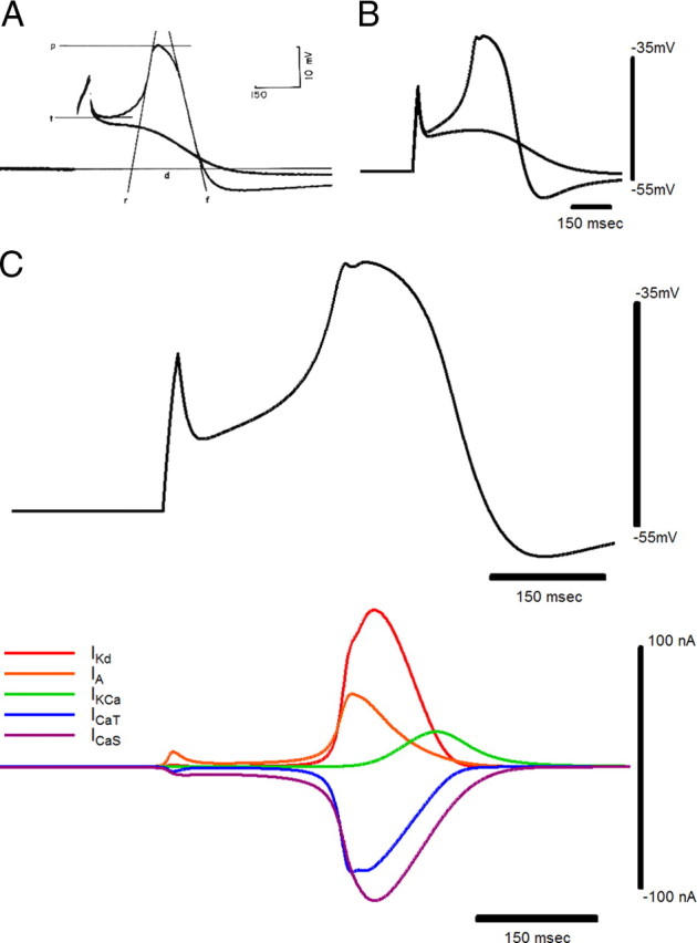
The driver potential response. Comparison of driver potential (p, peak; d, duration; t, threshold; r, line tangent to the maximum rate of rise; f, line tangent to the maximum rate of fall) and subthreshold responses in an anterior large cell of Portunus (A) (Tazaki and Cooke, 1979b) with those in the large-cell model (B). Current pulses in the model: DP, 20 nA, 20 ms. Subthreshold, 17 nA, 20 ms. C, Currents in the large-cell soma model during a driver potential.
Effects of parameter variations on CG output
Currents in the model LC soma during the driver potential
To understand how coregulations of current conductances in the LC could preserve output, we first investigated the activity and contributions of each ionic current in the LC soma to the driver potential shape. During the initial latency to the driver potential, the slow calcium current ICaS and the early outward current IA were the most prominent currents, opposing one another (Fig. 2C). During the later depolarizing phase of the driver potential, all LC soma currents except for IKCa activated, and ICaS and IKd were the most prominent currents. During the peak of the driver potential, ICaT and IA began to inactivate before the inactivation of ICaS and IKd. Finally, IKCa activated and reached its peak during the repolarization of the driver potential and the inactivation of the four remaining currents. To test how varying the maximal conductances of the LC currents affected the driver potential, we elicited driver potentials in cell models with various combinations of maximal conductances by setting the sodium conductance to zero in each case and injecting a 40 nA, 20 ms current pulse into the LC soma compartment. This current amplitude was chosen for its ability to elicit driver potentials in the largest number of conductance combinations, whereas current pulses of this duration with varying amplitudes (Fig. 3A) as well those with varying durations and amplitudes (Fig. 3B) were found to produce nearly identical driver potentials in a given LC model.
Figure 3.
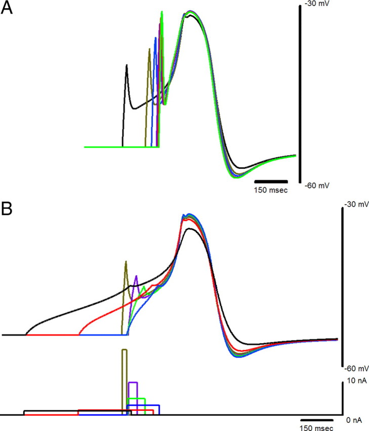
Driver potential form in the canonical large-cell model did not change significantly for different stimulus amplitudes or durations. A, Driver potential responses to 20 ms current injections ranging from 20 to 50 nA at 5 nA steps are overlaid with their peak voltages aligned. Longer latencies to the peak voltage correspond to weaker current injections. The trace with the lowest peak and least hyperpolarized afterpotential corresponds to a stimulus of 20 nA, which was just above threshold for a 20 ms current pulse. B, Driver potential responses (top) to current pulses (bottom) of varying duration with sufficient amplitudes to evoke full responses. Identical colors have been used for the stimulus and the corresponding membrane potential response.
Covariation of GCaT and GKd preserved driver potential form
Covarying GKd and GCaT in a pairwise manner while all other maximal conductances were held at their nominal values (Table 1) revealed that the overall form of the driver potential was best preserved when they were changed in equal proportion. To investigate how these currents could balance one another to preserve output, we evaluated the peak voltage and duration of the driver potential, two of its primary features, as only GCaT and GKd were varied (Fig. 4A). Increasing GCaT alone depolarized the peak of the driver potential and decreased its duration, while increasing GKd alone had the opposite effect on these two measurements. When these maximal conductances were varied in equal proportions, the duration was preserved, and varied by <7% of its nominal value over a fivefold range of parameter values. The peak voltage, in contrast, was best preserved when GCaT was varied in a nonlinear relationship to GKd, requiring somewhat larger increases in GCaT to balance increases of GKd to high values; however, varying GCaT and GKd in the same linear manner that preserves the DP duration changed the peak by <20% of its nominal value over the large range. This finding is consistent with the fact that more than two parameters must be varied to preserve two independent characteristics of a model neuron, which is shown clearly by Olypher and Calabrese (2007). Figure 4B shows a comparison of generated driver potential responses in the model when GCaT and GKd were varied together by onefold, twofold, threefold, fourfold, and fivefold increases in each. The initial latency to the driver potential decreased, but the form of the driver potential was preserved. Figure 4C shows the χ2 values for the driver potential (see Materials and Methods) for the GKd and GCaT adjustments indicated on the X and Y axes with all other conductances held at their nominal values. Note that a relative GCaT–GKd multiplier ratio near 1:1 preserved DP form, as reflected by a diagonal region in the GCaT–GKd space within which χ2 values approach a minimum.
Figure 4.
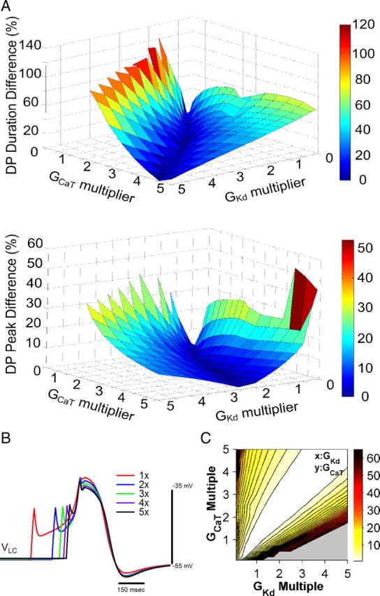
Variability of the driver potential response among varying maximal conductances for ICaT and IKd. A, Percentage change of the driver potential duration (top) and peak voltage (bottom) for changes to GKd and GCaT. The duration and peak are preserved for equal GCaT and GKd multiples. B, Comparisons of driver potentials in the large-cell model for multiples of GCaT and GKd of 1×, 2×, 3×, 4×, and 5× with peaks aligned. As the two maximal conductances increase, the onset of the driver potential upswing is advanced, although the form of the driver potential itself is mostly unchanged. C, χ2 values of driver potential characteristics in the large-cell model for x-fold variations in GKd and GCaT with all other model parameters held to their nominal values. The grayed-out region indicates combinations of conductances for which driver potentials were not produced in response to a 20 ms current injection or else the χ2 value was >100.
Balancing GCaS and GA was required for driver potential generation
When GA and GCaS were varied (while all other maximal conductances were held to their nominal values) (Table 1) in such a way that they balanced one another, the overall output was preserved (Fig. 5A). However, increasing GA without a compensatory increase in GCaS prevented the LC soma from generating driver potential responses to a 20 ms current injection (Fig. 5A–C,H). This limitation resulted from the inward current (primarily ICaS) being insufficient to overcome the outward current (primarily IA) near rest, rather than from a graded opposition to depolarization via current injection (see Materials and Methods). Conversely, increasing GCaS alone without also increasing GA unbalanced the LC currents near rest (primarily ICaS and IA), resulting in endogenous, repetitive driver potentials (Fig. 5E–G).
Figure 5.

χ2 values for the driver potential for pairwise x-fold variations of two maximal conductances while all other maximal conductances are held to their nominal values. The grayed areas indicate parameter combinations for which driver potentials were not elicited for a 20 ms, 40 nA pulse, endogenous driver potentials occurred regardless of stimulus strength, or the χ2 value was >100 (for ease of viewing). A, GCaS versus GA. B, GA versus GKCa. C, GCaT versus GA. D, GKCa versus GKd. E, GCaS versus GKd. F, GCaS versus GKCa. G, GCaS versus GCaT. H, GKd versus GA. I, GCaT versus GA.
Effect of other pairwise covariations
Linear coregulation of any pairs of maximal conductances alone other than GCaT–GKd and GCaS–GA (Fig. 5) did not preserve the driver potential features. For all pairwise covariations involving GA or GCaS, other than the two together, it was found that attempts to change a second conductance would not yield a driver potential once it was lost because of an increase to GA (Fig. 5B,C,H), and could not prevent spontaneous driver potential oscillations that arose because of an increase in GCaS (Fig. 5E–G). Also, although changes to GKCa caused modest shifts in driver potential characteristics (particularly during repolarization, when activation of IKCa is partially responsible for setting DP duration and the maximum AHP), these adjustments could not preserve DP form to compensate for changes to either GKd or GCaT (Fig. 5D,I).
Full variability of maximal conductances in the LC
To test whether correlations are preserved in a population in which all conductances are allowed to vary fully, we randomly chose model cells and retained or rejected them in a “sample set” by using their χ2 values (representing the fitness of the resulting driver potential) calculated from their measured driver potential characteristics (see Materials and Methods). Our rejection sampling technique generated ∼12,000 model cells that had a driver potential before 1000 were found to meet the criteria using our probabilistic sampling method. All cells in the resulting model dataset had driver potentials (20 ms pulse input) with the following characteristics (Table 6): DP duration of 254 ± 38 ms; DP peak of −33.5 ± 2.0 mV; maximum AHP of −60.3 ± 2.0 mV; maximum rate of rise of 0.29 ± 0.13 mV/ms; maximum rate of fall of 0.30 ± 0.08 mV/ms; and the rest potential was −53.2 ± 0.9 mV. Together, these data suggest that the model cells did produce DPs with features similar to that seen in the biological data. A histogram of the χ2 values for driver potentials in the sample set of LC models revealed that the distribution of values conformed well to a χ2 probability distribution with 2 df for χ2 > 2 (data not shown). However, for χ2 < 2, the distribution better resembled a χ2 distribution with 3 df. This result possibly reflects characteristics of the underlying model cells; it is possible that, although the maximal conductances were chosen from a uniform range of values, the resulting driver potential characteristics were not uniformly distributed in their χ2 values.
Table 6.
Measurements of LC driver potential features used for calculating χ2 values and for retaining or discarding model cells [biological set; data taken from Tazaki and Cooke (1979b)] and those determined from a sampled population of 1000 model cells (model set)
| DP feature | Biological set | Model set |
|---|---|---|
| Duration (ms) | 250 ± 50 | 254 ± 38 |
| Peak (mV) | −32 ± 3.0 | −33.5 ± 2.0 |
| AHP (mV) | −58 ± 3.0 | −60.3 ± 2.0 |
| Maximum rate of rise (mV/ms)a | 0.45 ± 0.15 | 0.29 ± 0.13 |
| Maximum rate of fall (mV/ms)a | 0.20 ± 0.12 | 0.30 ± 0.08 |
| Resting potential (mV)a | −53 ± 2.5 | −53.2 ± 0.9 |
aNote that these features of the LC soma were not used to constrain model cells.
Figure 6A shows two representative plots of the conductances in the 1000 model LC set in three dimensions: GKCa versus GCaT and GKd, and GCaT versus GCaS and GA. The conductances of the LC set agreed qualitatively with the conductance relationship findings in Figure 5. Namely, in models with low values of GKCa, lower values of GKd (Fig. 5D) and higher values of GCaT (Fig. 5I) were required to maintain a χ2 value near zero. Figure 6A, top, reinforces this idea; models with lower values of GKCa possessed lower values of GKd and higher values of GCaT. A similar three-way relationship is suggested in Figure 5: models with relatively high GCaT had higher values of GA (Fig. 5C) and lower values of GCaS (Fig. 5G) to preserve driver potential generation. This is demonstrated in Figure 6A, bottom, in which models with higher values of GCaT possessed higher values of GA and lower values of GCaS. As suggested by Figure 5, E and H, an opposite effect on values of GA and GCaS was seen with increased GKd; however, this effect was not as pronounced (data not shown). Changes to GKCa had little apparent effect on values in the GCaS–GA plane. Analysis of additional combinations of three conductances revealed relationships among conductances that agreed with those already presented here.
Figure 6.

Maximal conductance relationships in a population of randomly generated large-cell models constrained by χ2 values representing the model output. A, Distribution of model cells in two representative three-dimensional plots: GKCa, GCaT, and GKd (top), and GCaT, GCaS, and GA (bottom). The axes represent conductance values as multiples of those in the nominal model (Table 1). B, Coefficients of determination (R2 values) for conductance pairs in the model set. GCaS–GA boundaries for driver potential generation persisted throughout the model set. In all models, GKCa values partly determined the required balance of GCaT and GKd for driver potential preservation.
We hypothesized that model cells constrained by reported output data should possess maximal conductance correlations that are consistent with their biological counterparts. Correlations among the maximal conductances of the resulting model cells were quantified using coefficients of determination (R2). The R2 values for each pair of maximal conductances in the 1000 cell sample model set are shown in Figure 6B. Predominantly, these results are consistent with those found using only pairwise covariations of maximal conductances. A strong correlation between GCaS and GA was seen consistently (R2 = 0.76). This can be explained by the limiting condition that randomly chosen model cells must produce driver potential responses to a 20 ms current pulse. After the GCaS–GA pair, the next largest correlation was that for the GKd–GCaT pair (R2 = 0.27). This result is again consistent with the pairwise conductance variations presented above; a balance of IKd and ICaT preserved driver potential form even when the remaining three maximal conductances were allowed full freedom within the sampled range of values. The maximal conductances for IKd versus ICaT and ICaS versus IA for the cells in the model set are shown in Figure 7A. These conductances, as well as the correlations shown in Figure 6B, reveal that GCaT and GKd need not correlate as strongly as was necessary for GCaS and GA to preserve the driver potential. However, the maximal conductances shown in Figure 6A indicate that, for differing values of GKCa, different ratios of GCaT to GKd were required for driver potential preservation. When GKCa was allowed to vary, a relatively weak correlation between GCaT and GKd was evident, as in Figure 7A. However, when subsets of the 1000 model set were analyzed by tighter constraints on variations in GKCa (e.g., multipliers between a lower and upper bound), the R2 value for GCaT and GKd increased, becoming as high as 0.7 for GKCa values between four and five times its nominal value. In contrast, the boundaries for GCaS and GA that were required for driver potential generation showed little variation with other conductances, and as a result, a high R2 value was present for GCaS and GA in the entire 1000 model LC set. For no other maximal conductance pairs were R2 values found >0.1.
Figure 7.
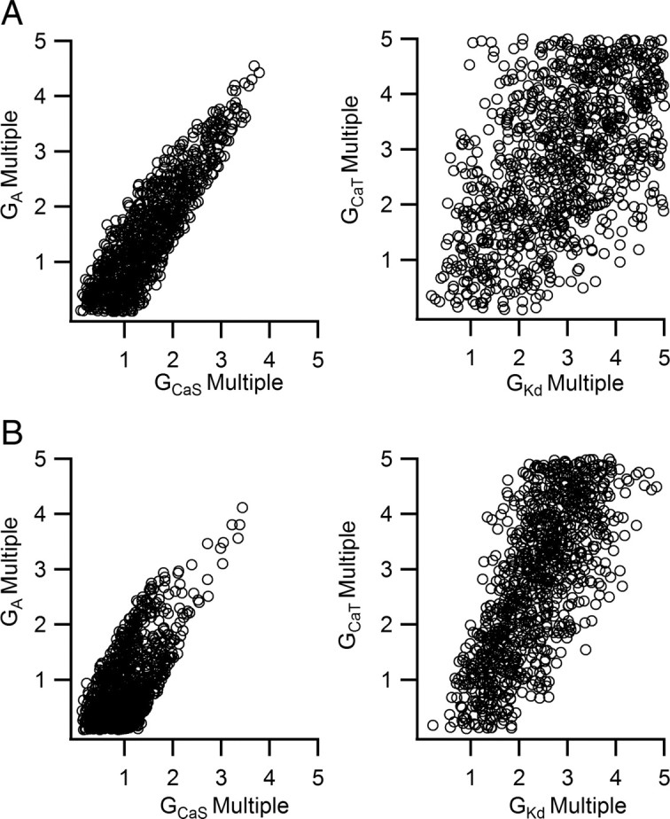
Relative maximal conductances (represented as a multiplier of the values in the nominal model) in a population of randomly generated large-cell models constrained by χ2 values representing the model output. A, Relative conductance values in a population chosen for biologically realistic output variances. B, Relative conductance values in a population chosen with one-third the biologically realistic SDs to simulate more stringent constraints on driver potential features. Model large cells generated using stricter requirements for driver potential form possess lower maximal conductances for ICaS and IA but possess values of GKd and GCaT that converge to a linear region of the two-dimensional space.
Manipulation of output distributions used for model selection
To test how the variability in the features used to filter model cell selection affects the relationships between maximal conductances in the resulting population, we explored a hypothetical scenario in which the features of the driver potential are more tightly constrained than indicated by Tazaki and Cooke (1979b) (i.e., that driver potential features deviate less from their averages). To simulate these conditions, two such scenarios were explored: the SDs for driver potential features were divided by factors of 2 and then 3. These changes increased the χ2 values for driver potentials in all model cells, decreasing the relative probabilities of survival for cell models with already large χ2 values. In these situations, R2 values for most pairs of maximal conductances increased somewhat, but most notably for GCaT versus GKd (R2 = 0.46 and R2 = 0.52 with all SDs divided by 2 and 3, respectively). This result is consistent with Figure 4; imposing a requirement of less variability on driver potential form necessitated a tighter ratio between GCaT and GKd. Additionally, a negative correlation emerged between GCaT and GKCa (R2 = 0.22 and then 0.32) as well as a small positive correlation between GCaT and GA (R2 = 0.17 and then 0.21). These correlations are consistent with the regions in the GCaT–GKCa and GCaT–GA planes that contain low χ2 values (Fig. 5C,I). However, the correlation between GCaS and GA actually decreased (R2 = 0.57 and then 0.43). The maximal conductances for ICaT versus IKd and ICaS versus IA in model cells constrained with SDs divided by 3 are shown in Figure 7B. Decreasing driver potential variability caused the range of maximal conductances of sampled model cells to become further constrained toward regions of the five-dimensional parameter space for which the χ2 values (representing a measure of divergence from mean driver potential characteristics) were very low. In the case of ICaT versus IKd, the maximal conductances of model cells were limited to a linear region, whereas for ICaS and IA, the conductances were lower without preserving such a strict linear relationship. A tight balance between GCaS and GA was required for driver potential generation, although the tighter constraints on specific driver potential features caused the desirable model candidates to cluster within a small region of values in the GCaS–GA plane. In this way, it is clear how imposing tighter constraints on driver potential form tends to better highlight correlations that serve to preserve the driver potential (e.g., GCaT vs GKd) and deemphasize others (e.g., GCaS vs GA).
This selection method does not account for the possibility that individual driver potential features are not independent of one another, a possibility that can typically be investigated if the full biological data set were available. For instance, parameter variations in the LC model suggested that the likelihood of a driver potential having a short duration would be greater if its peak is high. In an attempt to accommodate for such dependencies of the output features, we selected a new set of models using feature dependence as part of the model selection criteria. To do so, we used the more general sum of variations (X̄ −  )TS̄−1(X̄−) for the multivariate normal distribution, where X̄ and are the vectors of driver potential features and their mean values, and S̄ is their covariance matrix, whose diagonal elements are the variances of the individual driver potential features (Wasserman, 2004). To estimate the off-diagonal elements of S̄, covariances were calculated using driver potentials from the original set of 1000 model cells (for this population, S̄ = [1569.7, −24.9, 49.1; −24.9, 4.7, −1; 49.1, −1, 4.0] × 10−6). Then, using this general χ2 value calculation, a second set of 1000 model LCs was generated using the same sampling method. Interestingly, this second model set possessed driver potential characteristics very close to the first model set: duration, 251 ± 35 ms; peak, −33.0 ± 1.8 mV; AHP, −59.4 ± 1.7 mV; rate of rise, 0.33 ± 0.16 mV/ms; rate of fall, 0.28 ± 0.08 mV/ms; resting potential, −53.3 ± 1.0 mV. The maximal conductance correlations measured from this set of model cells were also similar: R2 = 0.55 for GCaS versus GA, R2 = 0.30 for GCaT versus GKd, and all other values <0.1. Also, similar to the case discussed above, the effect of reduced variability in driver potential features (by modifying S̄) can be investigated by reducing the elements of S̄ appropriately. These results are similar to those obtained with the first model set indicating that including the interdependence of output features suggested by the LC models does not significantly change our findings. Tazaki and Cooke (1979b) report only the means and variances of their biological dataset. If all the data are available, the covariance matrix can be generated using the entire set of biological driver potential characteristics. Alternatively, a probability distribution function can be empirically determined from these data, to avoid having to assume that the data follow a multivariate normal distribution.
Features of the multidimensional parameter space
Our analysis of the dependence of χ2 values on conductances considered two-dimensional versions of the multidimensional conductance space as shown in Figures 4C and 5. The plots show that with stricter constraints on allowable χ2 values (i.e., lower SD values), the shapes of the permissible spaces for conductances changes differently for different pairs of conductances, providing insights into the underlying mechanisms as we describe below.
If the ranges for the conductances are tightly constrained (around the nominal model) (i.e., if a relatively smaller parameter space is selected), then correlations among conductances might not be evident. For instance, if the conductance space of GKd and GCaT (around the nominal model), from which the 1000 cell model population is sampled, is reduced by 50% (i.e., a range of 0.5- to 2-fold the nominal values), then the correlation between the parameters drops from 0.27 to 0.04. Similarly, reducing the sampled conductance ranges for both GA and GCaS by 50% resulted in the correlation between the parameters dropping from 0.76 to 0.51. These results suggest that correlations among parameters, if they exist, will be evident only if the parameter space studied has sufficiently large ranges.
If, however, the features of the driver potential were more tightly constrained [e.g., by selecting smaller SDs for the output features (see above)], some correlations become stronger and others weaker. For instance, reducing the SD of the driver potential by a factor of 3 in sampled model LCs resulted in a lower correlation between GCaS and GA (0.43, as opposed to 0.76). This result seems counterintuitive, given that a balance between these two conductances is required in the model for driver potential generation. But Figure 5A suggests that this may be a consequence of the change in shape of the “permissible χ2” space in the GCaS–GA plane; a functional correlation is seen when χ2 is loosely constrained (yellow space), but not when it is more tightly constrained (white space). However, with the same stricter constraint on output features, the correlation between GKd and GCaT increased, from R2 = 0.27 to 0.52. This is consistent with the change in the shape of the permissible χ2 when covarying these conductances. As shown in Figure 4C, when model cells are constrained by increasingly stringent sampling (low χ2, white space), the shape of the permissible χ2 space reveals a sharpened correlation. This difference highlights the roles of these two pairs of currents as suggested by the model; ICaS and IA can preserve driver potential generation but not its form, and so do not correlate strongly under tight constraints based on DP form; however, the effects of ICaT and IKd are negligible around rest but need to balance one another to preserve driver potential form. This suggests that the geometrical shape of these permissible regions can provide information about correlations among the corresponding conductances.
Discussion
We constructed a biologically realistic computational model of the crustacean CG consisting of a large and small cell pair to test the hypothesis that coregulation of maximal conductances in the LC soma could preserve its driver potential. The present investigation was inspired by a molecular study of the CG of C. borealis in which mRNA transcripts of LCs that encode for ion channel proteins were measured, revealing correlations between transcript numbers for many genes (Tobin et al., 2009). The CG network model was developed from biological CG data, especially the comprehensive studies performed by Tazaki and Cooke (Tazaki, 1971; Tazaki and Cooke, 1979a,b,c, 1983a,b, 1986, 1990; Cooke, 2002), and this model reproduced many features of the CG output, in particular the driver potential response of the LC, spontaneous bursting of the synaptically coupled large and small cells, and various essential features of both types of output. In addition to thoroughly characterizing the contribution of each ionic current to the properties of the driver potential, we varied the maximal conductances of the ionic currents in the LC soma and investigated relationships between the maximal conductances that preserved the form of the LC driver potential. We then investigated how constraining maximal conductances of the model using reported information about the output of LCs (Tazaki and Cooke, 1979b) revealed required covariations between maximal conductances in the LC model.
ICaS and IA are correlated for driver potential generation
A balance of the maximal conductances of ICaS and IA was required for the model to produce nonendogenous driver potentials in response to a short, strong current injection. A strong relationship between ICaS and IA is evident both from the χ2 values when these two conductances were covaried in a model (Fig. 5A) and from the pairwise correlation found in the population of randomly chosen models that were constrained by LC output (Fig. 6). This relationship was not disturbed by variations in other maximal LC conductances. However, in a population of models chosen with more tight constraints on output, the correlation between GCaS and GA decreased. In a study of a lateral pyloric (LP) STG neuron model (Taylor et al., 2009), a boundary determined by maximal conductances of both ICa and IA appears to restrict the ability of the model to produce acceptable LP-like behavior, although a strong correlation between these two parameters may not be necessary. Thus, the model results predict that the maximal conductances of ICaS and IA must balance via linear coregulation to preserve the generation of driver potentials in LCs, although a tight coregulation among them does not appear to be necessary.
ICaT and IKd coregulate to preserve the driver potential
As indicated by mRNA data, levels of shab, a gene that encodes for IKd channels, are strongly correlated (R2 = 0.83) to levels of cacophony, a gene that encodes for a channel that carries a calcium current with unknown properties (Tobin et al., 2009). We used the LC model to explore relationships between IKd and calcium currents that preserve electrical output. The model demonstrates how balancing the maximal conductances of ICaT and IKd would maintain driver potential characteristics. Individually varying GCaT and GKd produced opposing actions on the driver potential peak and width. Covarying these conductances preserved the driver potential form (Fig. 4). In a population of models chosen to match biological means and variability in driver potential characteristics, levels of GCaT and GKd were correlated. This relationship persisted despite variations in other maximal LC conductances; however, variations to GKCa caused the required ratio of GCaT to GKd to shift, causing a lower overall correlation between these two parameters when the conductances of all 1000 random models were considered. Furthermore, when more stringent requirements for driver potential form were imposed on the population of models, the correlation between these two maximal conductances increased. Such findings demonstrate that GCaT and GKd can functionally balance to preserve driver potential output and they predict that, if driver potential features are tightly constrained in C. borealis using this set of ionic currents, a strong correlation should emerge for the relative abundances of channels carrying ICaT and IKd. Thus, in addition to the prediction that GCaT and GKd coregulate to preserve driver potential form, the model also suggests that the cacophony gene in LCs encodes channels that carry an ICaT-like current.
It is possible that a single-channel type with complex kinetics could account for both ICaS and ICaT in this system. However, our data demonstrate that these two currents have distinct and independent influences on the driver potential. Furthermore, randomly generated models constrained by LC output produced a relatively weak negative correlation between GCaS and GCaT. These data are therefore consistent with the idea of independent sources of ICaT and ICaS type conductances. If cacophony does indeed encode for channels carrying both ICaS and ICaT, a balance between these two currents may exist through a secondary mechanism to regulate cell output such as splice variants or posttranslational modification.
Similar forms of compensation among ionic conductances that stabilize output have been reported in biological experiments. For example, cultured Drosophila neurons that lack significant levels of ICa undergo a homeostatic decrease in IKCa and a subsequent increase in IA thought to stabilize output (Peng and Wu, 2007). Additionally, STG neurons of the spiny lobster undergo compensatory upregulation of IH when levels of an opposing A-type current are artificially upregulated (MacLean et al., 2003, 2005). However, modeling-based approaches have suggested that such correlated conductances can maintain functionally relevant output, but are not necessary. For example, our first approach is similar to that of MacLean et al. (2005), who used a conductance-based model with systematic covarying of conductances, to indicate that increasing IA or IH singly changes the output of bursting cells, but increasing them together maintains target neuronal activity. Conversely, our second approach is similar to that of Taylor et al. (2009), who created a population of model neurons that encompasses variability akin to a biological population, to suggest that such correlations among conductances are not necessary to generate conserved functional output. By combining these two approaches in the same study, we obtained results consistent between the two methods, namely that correlated conductances maintain driver potential features in large cells. Our bilateral approach is strongly suggestive that correlations measured in ion channel mRNA, particularly that of cacophony–shab (ICa and IKd), (Tobin et al., 2009), exist because they are functionally relevant in this system.
Conclusions
Biophysical models of neurons and neuronal networks developed using biological data typically capture nominal behavior. More recently, it has become clear that production of a given neuronal output via a single, canonical set of underlying properties (a population mean per se) may be less reflective of true biological populations (for a review of this idea, see Marder et al., 2007). Motivated by this emerging concept, if a specific output of a model is of interest, it is pertinent to ask the question, “Would another set of model parameters yield the same output?” The model developed in the present study, for instance, was motivated by such a question, “In the presence of the large variability in mRNA expression for CG cells, are there multiple maximal conductance sets that might provide the same driver potential, and if so, what relationships govern such sets?” As cited in Materials and Methods, we adapt an approach reminiscent of “rejection sampling” (Robert and Casella, 2004) in a novel approach to sample the multidimensional parameter space and develop metrics to quantify the driver potential features. In short, a canonical model was developed to match existing biological data. Random values were selected for parameters whose impact on model behavior was to be examined (in this case, the effect of maximal conductances on LC driver potential). Models were generated from the random parameter sets and the model outputs were characterized for key outputs (in this case, peak voltage, duration, and maximum AHP of the driver potential) using a sum of standardized variations. Models were retained or discarded using an assumed probability distribution function (in this case, a χ2 distribution with 2 df) until the desired sample size was obtained (in this case, 1000 cell models). The primary result of our method is the production of a randomly sampled set of model cells constrained by a biologically measured distribution of output data. In this way, cell models possessing output considered to be an outlier in biological distributions will also be outliers in the sample model set. Although the resulting model cells in the present study were used to quantify correlation coefficients between different pairs of maximal conductances, the model sets could have been investigated to evaluate other biological features such as action potential height, width, firing rates, slow-wave amplitudes, and burst periods. By allowing full variability of the model conductances, but constraining the population based on biologically accurate variability in output, we were able to assess how pairwise correlations could emerge in the face of more realistic biological variability (Marder et al., 2007).
Limitations
Although we have performed these experiments with a thorough treatment of the biological data at hand, limitations in the biological knowledge of the system leave three possibilities that may confound the specific results presented here. First, output preservation may not simply entail balancing maximal conductance, but also result from posttranslational mechanisms modifying channel kinetics. Although compensatory changes that stabilize neuronal output in the absence of changes in channel kinetics have been demonstrated in Drosophila neurons (Peng and Wu, 2007), homeostatic regulation may occur at multiple levels of processing. Second, the model assumes colocalization for all conductances known to generate the driver potential. Little is known about functional compartmentalization of channel types in these cells, and such localization would not be apparent from correlations between total mRNA transcripts for the cells. Third, coregulation of ion channel densities may serve additional purposes for maintenance of output or other cellular properties than investigated here. In the future, the reported CG model can be extended to include posttranslational and other relevant mechanisms as they become better understood biologically, and can then be used to study their effect on preserving output function.
Footnotes
This work was supported by National Institutes of Health Grant NS059255 (A.-E.T.), National Science Foundation (NSF) Grant IOB-0615160 (D.J.S.), and NSF Grant DGE-0440524 (S.S.N.). We thank Drs. Adam Taylor and Eve Marder for helpful comments and suggestions on a previous draft, and Dr. John Fresen for assistance with statistical concepts. We are also grateful to the anonymous reviewers for their insightful suggestions that helped improve this manuscript.
References
- Achard P, De Schutter E. Complex parameter landscape for a complex neuron model. PLoS Comput Biol. 2006;2:e94. doi: 10.1371/journal.pcbi.0020094. [DOI] [PMC free article] [PubMed] [Google Scholar]
- Berlind A. Spontaneous and repetitive driver potentials in crab cardiac ganglion neurons. J Comp Physiol A Neuroethol Sens Neural Behav Physiol. 1982;149:263–276. [Google Scholar]
- Berlind A. Heterogeneity of motoneuron driver potential properties along the anterior-posterior axis of the lobster cardiac ganglion. Brain Res. 1993;609:51–58. doi: 10.1016/0006-8993(93)90854-g. [DOI] [PubMed] [Google Scholar]
- Bower JM, Beeman D. Ed 2. New York: Springer-Verlag; 1998. The book of GENESIS: exploring realistic neural models with the GEneral NEural SImulation System. [Google Scholar]
- Buchholtz F, Golowasch J, Epstein IR, Marder E. Mathematical model of an identified stomatogastric ganglion neuron. J Neurophysiol. 1992;67:332–340. doi: 10.1152/jn.1992.67.2.332. [DOI] [PubMed] [Google Scholar]
- Bullock TH, Terzuolo CA. Diverse forms of activity in the somata of spontaneous and integrating ganglion cells. J Physiol. 1957;138:341–364. doi: 10.1113/jphysiol.1957.sp005855. [DOI] [PMC free article] [PubMed] [Google Scholar]
- Cooke IM. Reliable, responsive pacemaking and pattern generation with minimal cell numbers: the crustacean cardiac ganglion. Biol Bull. 2002;202:108–136. doi: 10.2307/1543649. [DOI] [PubMed] [Google Scholar]
- Fort TJ, Brezina V, Miller MW. Regulation of the crab heartbeat by FMRFamide-like peptides: multiple interacting effects on center and periphery. J Neurophysiol. 2007;98:2887–2902. doi: 10.1152/jn.00558.2007. [DOI] [PubMed] [Google Scholar]
- Golowasch J, Buchholtz F, Epstein IR, Marder E. Contribution of individual ionic currents to activity of a model stomatogastric ganglion neuron. J Neurophysiol. 1992;67:341–349. doi: 10.1152/jn.1992.67.2.341. [DOI] [PubMed] [Google Scholar]
- Günay C, Edgerton JR, Jaeger D. Channel density distributions explain spiking variability in the globus pallidus: a combined physiology and computer simulation database approach. J Neurosci. 2008;28:7476–7491. doi: 10.1523/JNEUROSCI.4198-07.2008. [DOI] [PMC free article] [PubMed] [Google Scholar]
- Hagiwara S, Bullock TH. Intracellular potentials in pacemaker and integrative neurons of the lobster cardiac ganglion. J Cell Physiol. 1957;50:25–47. doi: 10.1002/jcp.1030500103. [DOI] [PubMed] [Google Scholar]
- Hagiwara S, Watanabe A, Saito N. Potential changes in syncytial neurons of lobster cardiac ganglion. J Neurophysiol. 1959;22:554–572. doi: 10.1152/jn.1959.22.5.554. [DOI] [PubMed] [Google Scholar]
- Hartline DK. Impulse identification and axon mapping of the nine neurons in the cardiac ganglion of the lobster Homarus americanus. J Exp Biol. 1967;47:327–340. doi: 10.1242/jeb.47.2.327. [DOI] [PubMed] [Google Scholar]
- Hartline DK. Integrative neurophysiology of the lobster cardiac ganglion. Am Zool. 1979;19:53–65. [Google Scholar]
- Khorkova O, Golowasch J. Neuromodulators, not activity, control coordinated expression of ionic currents. J Neurosci. 2007;27:8709–8718. doi: 10.1523/JNEUROSCI.1274-07.2007. [DOI] [PMC free article] [PubMed] [Google Scholar]
- MacLean JN, Zhang Y, Johnson BR, Harris-Warrick RM. Activity-independent homeostasis in rhythmically active neurons. Neuron. 2003;37:109–120. doi: 10.1016/s0896-6273(02)01104-2. [DOI] [PubMed] [Google Scholar]
- MacLean JN, Zhang Y, Goeritz ML, Casey R, Oliva R, Guckenheimer J, Harris-Warrick RM. Activity-independent coregulation of IA and Ih in rhythmically active neurons. J Neurophysiol. 2005;94:3601–3617. doi: 10.1152/jn.00281.2005. [DOI] [PubMed] [Google Scholar]
- Marder E, Goaillard JM. Variability, compensation and homeostasis in neuron and network function. Nat Rev Neurosci. 2006;7:563–574. doi: 10.1038/nrn1949. [DOI] [PubMed] [Google Scholar]
- Marder E, Tobin AE, Grashow R. How tightly tuned are network parameters? Insight from computational and experimental studies in small rhythmic motor networks. Prog Brain Res. 2007;165:193–200. doi: 10.1016/S0079-6123(06)65012-7. [DOI] [PubMed] [Google Scholar]
- Mayeri E. Functional organization of the cardiac ganglion of the lobster, Homarus americanus. J Gen Physiol. 1973;62:448–472. doi: 10.1085/jgp.62.4.448. [DOI] [PMC free article] [PubMed] [Google Scholar]
- Maynard DM. Activity in a crustacean ganglion. II. Pattern and interaction in burst formation. Biol Bull. 1955;109:420–436. [Google Scholar]
- Olypher AV, Calabrese RL. Using constraints on neuronal activity to reveal compensatory changes in neuronal parameters. J Neurophysiol. 2007;98:3749–3758. doi: 10.1152/jn.00842.2007. [DOI] [PubMed] [Google Scholar]
- Peng IF, Wu CF. Drosophila cacophony channels: a major mediator of neuronal Ca2+ currents and a trigger for K+ channel homeostatic regulation. J Neurosci. 2007;27:1072–1081. doi: 10.1523/JNEUROSCI.4746-06.2007. [DOI] [PMC free article] [PubMed] [Google Scholar]
- Prinz AA, Billimoria CP, Marder E. Alternative to hand-tuning conductance-based models: construction and analysis of databases of model neurons. J Neurophysiol. 2003;90:3998–4015. doi: 10.1152/jn.00641.2003. [DOI] [PubMed] [Google Scholar]
- Prinz AA, Bucher D, Marder E. Similar network activity from disparate circuit parameters. Nat Neurosci. 2004;7:1345–1352. doi: 10.1038/nn1352. [DOI] [PubMed] [Google Scholar]
- Robert CP, Casella G. Monte Carlo statistical methods. New York: Springer; 2004. [Google Scholar]
- Schulz DJ, Goaillard JM, Marder E. Variable channel expression in identified single and electrically coupled neurons in different animals. Nat Neurosci. 2006;9:356–362. doi: 10.1038/nn1639. [DOI] [PubMed] [Google Scholar]
- Schulz DJ, Goaillard JM, Marder EE. Quantitative expression profiling of identified neurons reveals cell-specific constraints on highly variable levels of gene expression. Proc Natl Acad Sci U S A. 2007;104:13187–13191. doi: 10.1073/pnas.0705827104. [DOI] [PMC free article] [PubMed] [Google Scholar]
- Soto-Treviño C, Rabbah P, Marder E, Nadim F. Computational model of electrically coupled, intrinsically distinct pacemaker neurons. J Neurophysiol. 2005;94:590–604. doi: 10.1152/jn.00013.2005. [DOI] [PMC free article] [PubMed] [Google Scholar]
- Swensen AM, Bean BP. Robustness of burst firing in dissociated Purkinje neurons with acute or long-term reductions in sodium conductance. J Neurosci. 2005;25:3509–3520. doi: 10.1523/JNEUROSCI.3929-04.2005. [DOI] [PMC free article] [PubMed] [Google Scholar]
- Taylor AL, Goaillard JM, Marder E. How multiple conductances determine electrophysiological properties in a multicompartment model. J Neurosci. 2009;29:5573–5586. doi: 10.1523/JNEUROSCI.4438-08.2009. [DOI] [PMC free article] [PubMed] [Google Scholar]
- Tazaki K. The effects of tetrodotoxin on the slow potentials and spikes in the cardiac ganglion of a crab, Eriocheir japonicus. Jpn J Physiol. 1971;21:529–536. doi: 10.2170/jjphysiol.21.529. [DOI] [PubMed] [Google Scholar]
- Tazaki K, Cooke IM. Spontaneous electrical activity and interaction of large and small cells in cardiac ganglion of the crab, Portunus sanguinolentus. J Neurophysiol. 1979a;42:975–999. doi: 10.1152/jn.1979.42.4.975. [DOI] [PubMed] [Google Scholar]
- Tazaki K, Cooke IM. Isolation and characterization of slow, depolarizing responses of cardiac ganglion neurons in the crab, Portunus sanguinolentus. J Neurophysiol. 1979b;42:1000–1021. doi: 10.1152/jn.1979.42.4.1000. [DOI] [PubMed] [Google Scholar]
- Tazaki K, Cooke IM. Ionic bases of slow, depolarizing responses of cardiac ganglion neurons in the crab, Portunus sanguinolentus. J Neurophysiol. 1979c;42:1022–1047. doi: 10.1152/jn.1979.42.4.1022. [DOI] [PubMed] [Google Scholar]
- Tazaki K, Cooke IM. Topographical localization of function in the cardiac ganglion of the crab, Portunus sanguinolentus. J Comp Physiol A Neuroethol Sens Neural Behav Physiol. 1983a;151:311–328. [Google Scholar]
- Tazaki K, Cooke IM. Separation of neuronal sites of driver potential and impulse generation by ligaturing in the cardiac ganglion of the lobster, Homarus americanus. J Comp Physiol A Neuroethol Sens Neural Behav Physiol. 1983b;151:329–346. [Google Scholar]
- Tazaki K, Cooke IM. Currents under voltage clamp of burst-forming neurons of the cardiac ganglion of the lobster (Homarus americanus) J Neurophysiol. 1986;56:1739–1762. doi: 10.1152/jn.1986.56.6.1739. [DOI] [PubMed] [Google Scholar]
- Tazaki K, Cooke IM. Characterization of Ca current underlying burst formation in lobster cardiac ganglion motorneurons. J Neurophysiol. 1990;63:370–384. doi: 10.1152/jn.1990.63.2.370. [DOI] [PubMed] [Google Scholar]
- Tobin AE, Calabrese RL. Endogenous and half-center bursting in morphologically inspired models of leech heart interneurons. J Neurophysiol. 2006;96:2089–2106. doi: 10.1152/jn.00025.2006. [DOI] [PMC free article] [PubMed] [Google Scholar]
- Tobin AE, Cruz-Bermúdez ND, Marder E, Schulz DJ. Correlations in ion channel mRNA in rhythmically active neurons. PLoS One. 2009;4:e6742. doi: 10.1371/journal.pone.0006742. [DOI] [PMC free article] [PubMed] [Google Scholar]
- Turrigiano G, LeMasson G, Marder E. Selective regulation of current densities underlies spontaneous changes in the activity of cultured neurons. J Neurosci. 1995;15:3640–3652. doi: 10.1523/JNEUROSCI.15-05-03640.1995. [DOI] [PMC free article] [PubMed] [Google Scholar]
- Wasserman L. New York: Springer; 2004. All of statistics: a concise course in statistical inference. [Google Scholar]