Non-linear modeling was applied thoughtfully for risk prediction: the Prostate Biopsy Collaborative group

Abstract

Objective

We aimed to compare non-linear modelling methods for handling continuous predictors for reproducibility and transportability of prediction models.

Study Design and Setting

We analyzed four cohorts of previously unscreened men who underwent prostate biopsy for diagnosing prostate cancer. Continuous predictors of prostate cancer included prostate-specific antigen and prostate volume. The logistic regression models included linear terms, logarithmic terms, fractional polynomials of degree 1 or 2 (FP1 and FP2) or restricted cubic splines with 3 or 5 knots (RCS3 and RCS5). The resulting models were internally validated by bootstrap resampling, and externally validated in the cohorts not used at model development. Performance was assessed with the area under the ROC curve (AUC) and the calibration component of the Brier score (CAL).

Results

At internal validation models with FP2 or RCS5 showed slightly better performance than the other models (typically 0.004 difference in AUC and 0.001 in CAL). At external validation models containing logarithms, FP1 or RCS3 showed better performance (differences 0.01 and 0.002).

Conclusion

Flexible non-linear modelling methods led to better model performance at internal validation. However, when application of the model is intended across a wide range of settings, less flexible functions may be more appropriate to maximize external validity.

Introduction

Screening for prostate cancer is usually based on the level of the molecular marker prostate-specific antigen (PSA). The use of this marker results in a relatively low specificity with a substantial number of negative biopsies [1]. The number of unnecessary biopsies may be reduced by using prediction models that combine several patient characteristics as predictor variables to selectively identify patients at high risk of prostate cancer [2].

Many prediction models contain linear associations between risk of an outcome and continuous predictors. Prediction models predicting prostate cancer risk often describe the association between PSA and prostate cancer risk using a curved line, rather than a straight line, indicating that a linear association is not appropriate [3-6]. More advanced modeling has been used to describe non-linear associations [7]. However, the possible benefit of more flexible methods that can use more than one curve per line to model the shape of the association between predictor and outcome has been insufficiently studied. Two commonly suggested flexible classes of functions for modeling non-linear associations are fractional polynomials and restricted cubic splines (RCS) [8, 9]. Fractional polynomials include a restricted set of power transformations. A formal test procedure is available to select the most appropriate transformations [10]. The test procedure aims to strike a balance between obtaining a good model fit and building a parsimonious model. RCS uses cubic polynomials for modeling subsections of the data, joining the segments together at “knots”. At the extremes of the predictor range the association is restricted to a linear association to increase the stability of the resulting associations [8]. These flexible functions may describe the association between predictor and outcome better in the data under study, but may also lead to overfitting of the model for predictive purposes.

Overfitting of prediction models can be assessed with internal validation procedures, which quantifies the reproducibility of a prediction model [11, 12]. The reproducibility of a prediction model refers to the performance of the prediction model in patients from the same population used at model development. External validation is required to assess the transportability of a prediction model. Transportability refers to the ability of prediction models to give accurate predictions in patients which are different but plausibly related to the population used at model development [11].

We aimed to compare prediction models that include different terms and functions to describe the association of the continuous predictors PSA and prostate volume with prostate cancer risk. We used data from four large cohorts containing men who had not previously undergone biopsy. Reproducibility of the prediction models was studied using bootstrap resampling techniques applied to the same cohort used at model development, and transportability by applying the models developed in one cohort to the three cohorts not used at model development.

Patients & Methods

Patients

We analyzed individual patient data from the Prostate Biopsy Collaborative Group [7]. Two cohorts (the Netherlands [n=2,895] and Göteborg, Sweden [n=740]) were part of the European Randomized Study of Screening for Prostate Cancer [1]. The third cohort (Tyrol) contained men from Tyrol, Austria (n=5,644) who were invited to attend free-of-charge PSA-testing [13]. The fourth cohort was a clinical cohort from Cleveland (Ohio, USA: Cleveland Clinic Foundation, (CCF) [n=3,286]). All men were previously unscreened and received a biopsy to determine the presence of prostate cancer. Two patients were removed from the analysis due to a recorded prostate volume of 0 cc.

Methods

In each cohort we constructed prediction models based on logistic regression containing the continuous predictors PSA and transrectal ultrasound measured prostate volume. We considered four different methods for modeling the shape of the association between predictor and outcome: 1) linear associations between predictors and outcome, 2) logarithmic associations between predictors and outcome, 3) associations between predictors and outcome modeled using fractional polynomials of degree one (FP1) [9], 4) fractional polynomials of degree two (FP2), 5) associations between predictors and outcome modeled with RCS using three knots (RCS3) [14], and 6) RCS using five knots (RCS5). We note that proponents of fractional polynomials have suggested FP2 as the default modeling approach to address non-linearity in continuous predictors [9], while 5 knots are the default for RCS [8]. Both FP2 and RCS5 effectively use 4 df in the modeling process.

Fractional polynomials

Fractional polynomials provide a framework to formally incorporate the choice of transformations into the model building process [10]. Fractional polynomials consider a limited, but flexible, set of transformations to describe the association between predictor and outcome. A test procedure is available to select the most appropriate transformation, among a linear association, fractional polynomial of degree one and a fractional polynomial of degree two, striking a balance between good model fit and the available evidence of a non-linear association in the data [15].

Restricted cubic splines

RCS model the association between predictor and outcome using cubic polynomials (polynomials of order 3) and linear terms [14]. RCS require the placement of a number of knots along the predictor value range. Between two knots the association between predictor and outcome is modeled using a cubic polynomial, outside the two outer knots the association is restricted to a linear association. The estimated associations in each of the intervals are forced to connect smoothly at the knots. The number and placement of the knots need to be specified by the user. Usually 3 to 5 knots are sufficient to allow for complex associations between predictor and outcome. Default placements of the knots are based on percentiles of the predictor values. Three knots are commonly placed on the 10th, 50th and 90th percentile of the predictor value range, five knots are typically placed at the 5th, 27.5th, 50th, 72.5th and 95th percentile [8].

Model performance

For each model we assessed discrimination and calibration. Discrimination refers to the ability of a prediction model to distinguish between patients with and without the outcome and was quantified using the area under the receiver operating characteristic curve (AUC) [8]. Calibration refers to the agreement between the predicted probabilities and observed outcomes. The Brier score is defined as the mean squared error between the predicted probabilities and the observed outcomes and can be considered as an overall measure of model performance. The Brier score can be split into two parts: calibration and refinement, the latter being the same as discrimination [16]. We used the calibration component of the Brier score to complement the AUC measuring discrimination. To be able to split the Brier score into the two components we divided the range of predicted probabilities into intervals, such that each interval contained approximately 100 patients. We calculated the average predicted probability of all patients within an interval. Subsequently, we assigned this average probability to all patients within this interval as the predicted probability of prostate cancer. The same intervals were used for all models when validating in a specific cohort.

Reproducibility was studied by internally validating the developed prediction model, where bootstrapping was used to correct for optimism in the apparent model performance [17]. In the bootstrap procedure a bootstrap sample is generated by drawing patients with replacement from the original dataset. A prediction model is subsequently developed in the bootstrap sample. The decrease between estimated performance in the bootstrap sample and estimated performance in the original sample is the optimism. This is repeated a large number of times. The average optimism is subsequently subtracted from the original estimate of model performance to obtain an optimism-corrected performance estimate. Transportability was assessed for models developed in each of the four cohorts in the three cohorts not used in model development.

Heterogeneity between cohorts

To quantify heterogeneity in predictive effects between the datasets we performed a random effects meta-analysis on the regression coefficients of the log-transformed values of PSA and prostate volume. Heterogeneity was quantified by the heterogeneity variance estimated in the meta-analysis [18].

Modeling

All analyses were done using R 2.15.1 (R foundation, Vienna, Austria), where fractional polynomials are implemented in the mfp package and RCS are implemented in the rms package. For both fractional polynomials and RCS we used the default settings of the software. The testing procedure of fractional polynomials used a significance level of 0.05. The knots of the RCS functions were placed at the default locations. The meta-analysis was performed using the metafor package.

Results

The prevalence of prostate cancer at biopsy was higher in the clinical cohort CCF (39%) compared to the three population based European cohorts (around 27%, Table 1). PSA levels and prostate volume in the Rotterdam and CCF cohorts were slightly higher compared to the cohorts from Göteborg and Tyrol. The age distribution of patients was similar across all cohorts.

Table 1. Characteristics of the subjects undergoing a biopsy for the presence of prostate cancer in the four cohorts.

	Rotterdam	Göteborg	Tyrol	CCF
	n = 2,895	n = 740	n = 5,644	n = 3,286
Prostate Cancer (prevalence)	28%	26%	28%	39%
PSA (ng/ml) median (25p-75p)	5.0 (3.9-7.3)	4.7 (3.7-6.7)	4.2 (2.8-6.8)	5.8 (4.3-8.5)
Prostate volume (cm3) median (25p-75p) (%-missing values)	46 (35-60) (0.4%)	39 (30-51) (0.9%)	35 (27-46) (8.4%)	42 (30-58) (30%)
Age (years) median (25p-75p)	66 (62-70)	61 (58-64)	63 (57-68)	64 (58-69)

P: percentile

ng/ml: nanogram per milliliter

cm³: cubic centimeter

PSA: Prostate-specific antigen

In all models, non-linear modeling methods showed similar increasing associations between the presence of prostate cancer and PSA at commonly observed PSA values (Figure 1). Differences between the modeling methods were visible at the extremes of the PSA range. Using FP1 led to the selection of the logarithmic transformation for PSA in three cohorts and the square root in one (Appendix table 1). Using FP2 led once to the selection of two polynomials to model the association between PSA and prostate cancer risk (Tyrol).The association modeled by the RCS5 function showed some signs of local non-monotonicity in the CCF cohort. There was substantial and statistically significant heterogeneity (estimated heterogeneity variance: 0.27 (Appendix figure 1).

Figure 1.

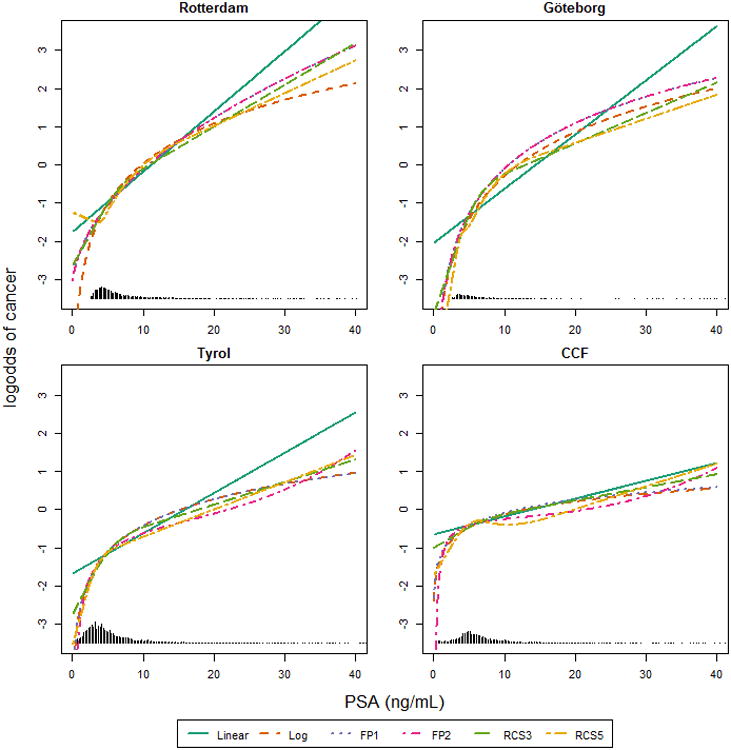
The association between PSA and the log-odds of cancer according to the different multivariable models. Prostate volume was set to 40 cm³. Linear: using linear terms; Log: using a logarithmic transformation; FP1: Fractional polynomial of degree 1; FP2: Fractional polynomials of degree 2; RCS3: restricted cubic splines with 3 knots; RCS5: restricted cubic splines with 5 knots.

For prostate volume all models described a similar decreasing association between prostate volume values and the presence of prostate cancer (Figure 2). Substantial differences became only apparent at low values of prostate volume, where the modeled association between prostate volume and prostate cancer risk showed a sudden drop in prostate cancer risk for low values of the predictors in the Tyrol cohort for FP2. The use of FP2 led to the selection of polynomials with two powers in three cohorts. The RCS5 functions showed again some local non-monoticity in the Göteborg and Tyrol cohort. The estimate of heterogeneity variance for the effect size of log-transformed volume was 0.37, which was statistically significant (See Appendix figure 2).

Figure 2.

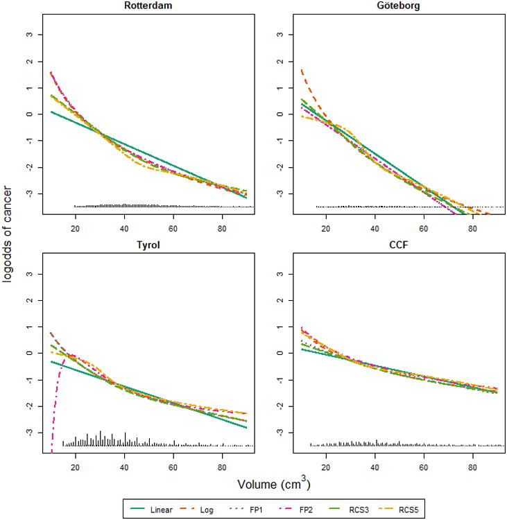
The association between prostate volume and the log-odds of cancer according to the different multivariable models. PSA was set to 4 ng/ml. Linear: using linear terms; Log: using a logarithmic transformation; FP1: Fractional polynomial of degree 1; FP2: Fractional polynomials of degree 2; RCS3: restricted cubic splines with 3 knots; RCS5: restricted cubic splines with 5 knots.

The differences in AUC between the four models were relatively small (typically 0.01, Table 2). Models containing linear terms typically had the lowest AUC, whereas models containing non-linear terms had higher AUCs at internal validation. Models containing FP2 or RCS5 typically had the highest AUC at internal validation. All other models showed similar AUC at internal validation. At external validation the AUCs of the models containing logarithmic terms, FP1 or RCS3 were typically highest. AUCs of models with linear term typically showed lower AUCs at external validation. Models using the more flexible transformations, i.e. FP2 or RCS5 typically showed lower AUCs compared to models containing logarithmic terms, FP1 or RCS3.

Table 2.

Discriminative ability (AUC) of the models, with 95% confidence interval, developed in one cohort (‘development set’) and validated in another cohort (‘validation set’). Higher AUC indicates better discrimination.

Validation set	Rotterdam
Transformation method	Linear	Log	FP1	FP2	RCS3	RCS5
Development set1
Rotterdam	0.745	0.747	0.749	0.749	0.748	0.751
Göteborg	0.740 [0.719, 0.761]	0.747 [0.726, 0.768]	0.743 [0.722, 0.764]	0.743 [0.722, 0.764]	0.743 [0.722, 0.764]	0.744 [0.722, 0.765]
Tyrol	0.745 [0.724, 0.766]	0.747 [0.726, 0.768]	0.747 [0.726, 0.768]	0.743 [0.722, 0.764]	0.746 [0.725, 0.767]	0.742 [0.721, 0.763]
CCF	0.740 [0.719, 0.761]	0.743 [0.746, 0.825]	0.742 [0.721, 0.763]	0.728 [0.729, 0.808]	0.744 [0.723, 0.765]	0.723 [0.702, 0.744]
	Göteborg
Rotterdam	0.783 [0.744, 0.823]	0.782 [0.742, 0.822]	0.782 [0.743, 0.822]	0.782 [0.743, 0.822]	0.784 [0.744, 0.824]	0.780 [0.740, 0.820]
Göteborg	0.787	0.785	0.791	0.791	0.789	0.791
Tyrol	0.785 [0.745, 0.824]	0.784 [0.744, 0.824]	0.784 [0.749, 0.829]	0.781 [0.741, 0.820]	0.782 [0.743, 0.822]	0.781 [0.741, 0.820]
CCF	0.785 [0.745, 0.824]	0.785 [0.746, 0.825]	0.789 [0.749, 0.828]	0.769 [0.984, 0.715]	0.787 [0.747, 0.826]	0.764 [0.724, 0.803]
	Tyrol
Rotterdam	0.692 [0.676, 0.708]	0.700 [0.685, 0.716]	0.694 [0.679, 0.710]	0.694 [0.679, 0.710]	0.697 [0.682, 0.713]	0.671 [0.655, 0.687]
Göteborg	0.686 [0.670, 0.702]	0.701 [0.686, 0.717]	0.700 [0.685, 0.716]	0.700 [0.685, 0.716]	0.701 [0.685, 0.716]	0.700 [0.684, 0.716]
Tyrol	0.684	0.695	0.695	0.699	0.693	0.699
CCF	0.686 [0.612, 0.651]	0.699 [0.684, 0.715]	0.702 [0.686, 0.718]	0.699 [0.684, 0.715]	0.695 [0.679, 0.711]	0.699 [0.683, 0.714]
	CCF
Rotterdam	0.626 [0.607, 0.646]	0.630 [0.611, 0.649]	0.628 [0.609, 0.648]	0.628 [0.609, 0.648]	0.629 [0.610, 0.649]	0.618 [0.599, 0.638]
Göteborg	0.631 [0.612, 0.651]	0.633 [0.613, 0.652]	0.633 [0.614, 0.653]	0.633 [0.614, 0.653]	0.635 [0.616, 0.654]	0.630 [0.611, 0.649]
Tyrol	0.629 [0.609, 0.648]	0.633 [0.613, 0.652]	0.633 [0.613, 0.652]	0.632 [0.613, 0.661]	0.633 [0.614, 0.652]	0.635 [0.616, 0.654]
CCF	0.628	0.634	0.636	0.639	0.632	0.640

¹Developed models contain the predictors PSA and prostate volume.

Underlined values indicate internal validation, performance was corrected for optimism using bootstrap (development and validation cohort is the same).

Log: Natural logarithm

FP1: Maximal allowed degree of Fractional polynomials 1

FP2: Maximal allowed degree of fractional polynomial 2

RCS3: Restricted cubic splines with 3 knots

RCS5: Restricted cubic splines with 5 knots

The calibration component of the Brier score was similar for all models containing non-linear terms at internal validation (Table 3). Models containing linear terms showed the worst calibration at internal validation (highest values for the Brier score). In contrast, the calibration component of the Brier score was typically best for models containing logarithmic terms, FP1 and RCS3 when externally validated, where models containing linear terms, FP2 or RCS5 showed poorer calibration. External validation of the model containing RCS5 in the CCF cohort typically led to the lowest calibration part of the brier score.

Table 3.

Calibration component of the Brier score of the model developed in one cohort (‘development set’) and validated in another cohort (‘validation set’). Lower values indicate better calibration.

Validation Set	Rotterdam							Göteborg
Transformation Method	Linear	Log	FP1	FP2	RCS3	RCS5		Linear	Log	FP1	FP2	RCS3	RCS5
Development Set1
Rotterdam	0.004	0.004	0.002	0.003	0.004	0.004	Rotterdam	0.011	0.013	0.009	0.009	0.011	0.010
Göteborg	0.007	0.005	0.006	0.005	0.005	0.006	Göteborg	0.012	0.011	0.013	0.015	0.013	0.013
Tyrol	0.009	0.007	0.007	0.008	0.006	0.005	Tyrol	0.012	0.014	0.014	0.008	0.010	0.009
CCF	0.023	0.018	0.021	0.034	0.019	0.017	CCF	0.037	0.034	0.040	0.034	0.034	0.031
Validation Set	Tyrol							CCF
Transformation Method	Linear	Log	FP1	FP2	RCS3	RCS5		Linear	Log	FP1	FP2	RCS3	RCS5
Development Set
Rotterdam	0.005	0.005	0.006	0.006	0.005	0.013	Rotterdam	0.016	0.017	0.017	0.017	0.017	0.017
Göteborg	0.003	0.005	0.005	0.005	0.004	0.007	Göteborg	0.029	0.029	0.031	0.031	0.028	0.033
Tyrol	0.004	0.002	0.002	0.002	0.002	0.002	Tyrol	0.020	0.015	0.015	0.015	0.015	0.015
CCF	0.025	0.019	0.020	0.020	0.022	0.016	CCF	0.004	0.004	0.003	0.003	0.003	0.002

¹Deveopd models contain the predictors PSA and prostate volume.

Underlined values indicate internal validation, performance was corrected for optimism using bootstrap (development and validation cohort is the same).

FP1: Maximal allowed degree Fractional polynomials 1

FP2: Maximal allowed degree of fractional polynomial 2

RCS3: Restricted cubic splines with 3 knots

RCS5: Restricted cubic splines with 5 knots

Discussion

We studied different terms and functions to model the known nonlinear association of PSA and prostate volume with prostate cancer risk. Flexible non-linear modelling methods, such as FP2 and RCS5, led to better reproducibility of the prediction model. However, transportability of the prediction models to other settings was better guaranteed when the transformations were restricted to less flexible functions, such as the logarithm, FP1 or RCS3. Models containing linear terms showed the poorest performance.

Internal validation was performed with bootstrapping techniques to assess the reproducibility of the developed prediction models [12]. We recognize that the development populations may be quite similar to the validation populations. In that case, reproducibility is assessed in the validation populations rather than transportability, which requires that the validation population is quite different from the development population [11]. Possible measures that can be used to quantify similarity are the mean and standard deviation of the linear predictor of the validated prediction model estimated in the development and validation populations [19]. Further, a low discriminative ability of a model predicting whether a patient is a member of the development or validation population indicates similar populations. As expected these measures indicated that the Rotterdam and Göteborg cohorts were rather similar. Validating a model that was developed in the Rotterdam cohort, in the Göteborg cohort can therefore be seen as close to evaluating the reproducibility of the prediction model. These measures also indicated that the clinical cohort CCF was much different from the population cohorts: the mean linear predictor was higher (-0.46 versus (-1.33 - -1.06) and the spread of the linear predictor smaller (0.46 versus (0.82-1.32)) compared to the population cohorts. Therefore we truly evaluated transportability when validating a prediction model developed in one of the other cohorts in the CCF cohort. Indeed, the difference in model performance between models containing logarithmic terms and RCS with five knots was smaller when the models were validated in cohorts more similar to the development cohort. These findings support the notion that modeling the association between predictors and outcome using flexible functions such as FP2 or RCS5 yields better reproducibility of a prediction model, while using a simple transformation such as the logarithm, FP1 or RCS3 provides better transportability. These findings are in line with previous studies showing that optimizing models for one population might degrade their performance in other populations [20].

Validation results, in terms of calibration, of the models developed in one of the population cohorts (Rotterdam, Göteborg and Tyrol) in CCF, and vice versa, were typically rather poor. This was mainly due to systematic underestimation of prostate cancer risk of the models developed in the population cohorts, as reflected in calibration-in-the-large values well above 0. Calibration-in-the-large indicates whether predictions are systematically over- or under-estimated, and is ideally equal to zero. Furthermore, the calibration slope of the models developed in the population cohort and validated in CCF were far below one, indicating that the predictor effects in these models were too extreme. Predictions by the model containing RCS5 were typically more extreme and slightly higher compared to models containing other terms. This resulted in a relatively good performance when externally validating the model in the CCF cohort were risks were systematically underestimated.

We found substantial heterogeneity in effects in a meta-analysis of the regression coefficients of the models containing logarithmic terms. The shape of the modelled associations between predictors and outcome using FP2 or RCS5 were also different between cohorts (Figures 1 and 2). This heterogeneity may explain the disappointing external performance of the models containing FP2or RCS5. Both FP2 and RCS5 are flexible functions that are able to follow the data closely when fitting a prediction model. Our study illustrates that these flexible functions may lead to a relative large drop in model performance at external validation in the presence of heterogeneity between development and validation populations. Restricting the modelled associations to a less flexible function, which is less sensitive to the particularities of one cohort, will give better results at external validation in this situation. This was observed when externally validating the prediction models containing a logarithmic transformation, FP1 or RCS3.

Modeling non-linear associations between predictors and outcome had a larger impact on the calibration of the prediction model. The AUC is based on the ranks of the predictions from a model. Hence by definition, univariable models with linear and logarithmic transformations, lead to the same AUC since both are monotonic increasing. This lack of sensitivity of the AUC to monotonic transformations of predictors is likely to extend to models with more than one predictor. Although a difference of 0.002 in the calibration part of the Brier score seems small, this indicates that on average predictions of one model were 5% more off than predictions of the other model.

Remarkably, the discriminative abilities of the models that were externally validated in the Göteborg cohort were higher than the discriminative abilities at internal validation. A change in AUC might be caused by different predictor effects or a difference in case-mix between the development and validation cohort [21]. These can be disentangled by using the case-mix corrected AUC and the standard deviation of the linear predictor. These revealed that the difference in AUC at internal and external validation of the models developed in the Rotterdam cohort were caused by a difference in case-mix. For the Tyrol and the CCF cohort the difference in AUC was mainly caused by a difference in predictor effects. It was also found that the lower AUC of the model developed in the CCF cohort was due to a more homogeneous population compared to the other cohorts, quantified by the spread of the linear predictors of the patients in the CCF cohort.

The observed associations between predictors and outcome only diverged at the extremes of the distribution of predictor values (Figure 1 and 2). This was reflected in the similar overall performance of models incorporating non-linear terms. The small difference in predictive performance of FP and RCS functions is in line with various simulation studies comparing these two methods to others [22, 23].

Sudden changes in prostate cancer risk estimated by models containing fractional polynomials at the extremes of the predictor value range may be caused by a small number of data points. These points may have a high leverage on the selected transformation [24]. It has been proposed to apply a transformation to the predictor values to reduce the leverage of these extreme points. This transformation is similar to double truncation or winsorising the predictor values [17]. Such a stabilizing procedure is conceptually related to restricting the association between predictors and outcome to a linear term at the extremes of the predictor value range and the concept of ‘shrinkage’ to achieve better predictions [25].

When developing a prediction model it is often a priori reasonable to expect a dose-response relationship between predictors and the outcome. Using flexible non-linear modelling methods however may lead to local non-monotonicity's defying the expected dose-response relationship. This can indicate that the association models particularities of the data at hand and can negatively impact external validity of the prediction model.

The use of a logarithmic transformation for a predictor is sometimes motivated by a skewed distribution of predictor values. We note that the use of a transformation should be motivated by a better fit in the prediction model rather than to deal with skewness in the predictor values. Sometimes a predictor with a skewed distribution can still best be modeled by a linear term in a regression model [26, 27].

In this study we modeled the association between prostate cancer risk and two predictors (PSA and prostate volume) and only considered using RCS and FP for both predictors. Restricting the use of RCS or FP for only one predictor in the prediction model might improve the performance of models containing RCS or FP functions at external validation. Furthermore, other predictors might bias the shape of the association between these predictors and prostate cancer risk. When we developed the models with adjustment for age and the result of a digital rectal exam, we found similar results.

While for both predictors, PSA and prostate volume, a logarithmic transformation seemed appropriate, other predictors might show different associations with prostate cancer risk. Flexible transformations, including FP and RCS, may be appropriate to model this association. External validation of the found association is necessary to assess transportability outside of settings where the model was developed. It may not be sufficient to only perform internal validation, which addresses reproducibility rather than transportability [11], if a broad interpretation is given to a predictor – outcome association.

In conclusion, our results illustrate that the choice of non-linear modelling method has a different impact on the reproducibility and transportability of a prediction model. Simple transformations, such as the logarithmic transformation or fractional polynomials and RCS with limited flexibility, may show adequate transportability. The choice of non-linear modeling method may therefore depend on the intended application of the prediction model. Simple transformations may be more appropriate when the model is applied across diverse patient populations. More advanced transformation methods may be more suitable when the prediction model will only be applied to patients similar to the development population.

Supplementary Material

1

Figure 1. Forest plot of estimated effect sizes of log2(PSA)

2

Figure 2. Forest plot of estimated effect sizes of log2(prostate volume)

3

Table 1. Powers of fractional polynomials selected with closed test procedure, as implemented in the mfp function in R software. (0 corresponds to the logarithmic transformation). FP1: fractional polynomials of degree 1; FP2: fractional polynomial of degree 2.

Key Findings.

Allowing a greater flexibility in the form of the association between continuous predictors and outcome in a prediction model leads to better reproducible results, but the transportability of such models may be poorer compared to models with simpler transformations.

What is known and what does this add.

Considering non-linear associations between continuous predictors and outcome may improve the performance of prediction models. However little is known about the relationship between the modelling of non-linear relationships and the reproducibility and transportability of a prediction model. We illustrated that more flexible functions could lead to a suboptimal performance at external validation. Restricting the modelled associations to less flexible functions, which are less sensitive to the particularities of one cohort, showed better results at external validation, or an increased transportability. This article provides new understandings and insights in how to apply these methods in a sensible way.

Implications.

Restricting the flexibility of the non-linear modelling method is preferred when we aim to apply a prediction model across a range of settings.

References

- 1.Schroeder FH, Hugosson J, Roobol MJ, Tammela TLJ, Ciatto S, Nelen V, et al. Screening and Prostate-Cancer Mortality in a Randomized European Study. New Engl J Med. 2009;360:1320–8. doi: 10.1056/NEJMoa0810084. [DOI] [PubMed] [Google Scholar]
- 2.Schroder F, Kattan MW. The comparability of models for predicting the risk of a positive prostate biopsy with prostate-specific antigen alone: A systematic review. Eur Urol. 2008;54:274–90. doi: 10.1016/j.eururo.2008.05.022. [DOI] [PubMed] [Google Scholar]
- 3.Carlson GD, Calvanese CB, Partin AW. An algorithm combining age, total prostate-specific antigen (PSA), and percent free PSA to predict prostate cancer: results on 4298 cases. Urology. 1998;52:455–61. doi: 10.1016/s0090-4295(98)00205-2. [DOI] [PubMed] [Google Scholar]
- 4.Finne P, Auvinen A, Aro J, Juusela H, Määttänen L, Rannikko S, et al. Estimation of Prostate Cancer Risk on the Basis of Total and Free Prostate-Specific Antigen, Prostate Volume and Digital Rectal Examination. Eur Urol. 2002;41:619–27. doi: 10.1016/s0302-2838(02)00179-3. [DOI] [PubMed] [Google Scholar]
- 5.Thompson IM, Ankerst DP, Chi C, Goodman PJ, Tangen CM, Lucia MS, et al. Assessing Prostate Cancer Risk: Results from the Prostate Cancer Prevention Trial. Journal of the National Cancer Institute. 2006;98:529–34. doi: 10.1093/jnci/djj131. [DOI] [PubMed] [Google Scholar]
- 6.Roobol MJ, van Vugt HA, Loeb S, Zhu X, Bul M, Bangma CH, et al. Prediction of prostate cancer risk: the role of prostate volume and digital rectal examination in the ERSPC risk calculators. European urology. 2012;61:577–83. doi: 10.1016/j.eururo.2011.11.012. [DOI] [PubMed] [Google Scholar]
- 7.Vickers AJ, Cronin AM, Roobol MJ, Hugosson J, Jones JS, Kattan MW, et al. The Relationship between Prostate-Specific Antigen and Prostate Cancer Risk: The Prostate Biopsy Collaborative Group. Clinical Cancer Research. 2010;16:4374–81. doi: 10.1158/1078-0432.CCR-10-1328. [DOI] [PMC free article] [PubMed] [Google Scholar]
- 8.Harrell FE. Regression Modeling Strategies: With Applications to Linear Models, Logistic Regression, and Survival Analysis. New York: Springer; 2001. [Google Scholar]
- 9.Royston P, Sauerbrei W. Multivariable Model - Building: A Pragmatic Approach to Regression Anaylsis based on Fractional Polynomials for Modelling Continuous Variables. Chichester: Wiley; 2008. [Google Scholar]
- 10.Royston P, Altman DG. Regression Using Fractional Polynomials of Continuous Covariates: Parsimonious Parametric Modelling. Journal of the Royal Statistical Society Series C (Applied Statistics) 1994;43:429–67. [Google Scholar]
- 11.Justice AC, Covinsky KE, Berlin JA. Assessing the Generalizability of Prognostic Information. Annals of Internal Medicine. 1999;130:515–24. doi: 10.7326/0003-4819-130-6-199903160-00016. [DOI] [PubMed] [Google Scholar]
- 12.Steyerberg EW, Harrell FE, Jr, Borsboom GJJM, Eijkemans MJC, Vergouwe Y, Habbema JDF. Internal validation of predictive models: Efficiency of some procedures for logistic regression analysis. Journal of Clinical Epidemiology. 2001;54:774–81. doi: 10.1016/s0895-4356(01)00341-9. [DOI] [PubMed] [Google Scholar]
- 13.Bartsch G, Horninger W, Klocker H, Pelzer A, Bektic J, Oberaigner W, et al. Tyrol Prostate Cancer Demonstration Project: early detection, treatment, outcome, incidence and mortality. BJU International. 2008;101:809–16. doi: 10.1111/j.1464-410X.2008.07502.x. [DOI] [PubMed] [Google Scholar]
- 14.Harrell FE, Lee KL, Pollock BG. Regression Models in Clinical Studies: Determining Relationships Between Predictors and Response. Journal of the National Cancer Institute. 1988;80:1198–202. doi: 10.1093/jnci/80.15.1198. [DOI] [PubMed] [Google Scholar]
- 15.Ambler G, Royston P. Fractional polynomial model selection procedures: investigation of type i error rate. Journal of Statistical Computation and Simulation. 2001;69:89–108. [Google Scholar]
- 16.Sanders F. On Subjective Probability Forecasting. Journal of Applied Meteorology. 1963;2:191–201. [Google Scholar]
- 17.Steyerberg EW. Clinical Prediction Models: A Practical Approach to Development, Validation, and Updating. New York: Springer-Verlag New York; 2009. [Google Scholar]
- 18.DerSimonian R, Laird N. Meta-analysis in clinical trials. Controlled Clinical Trials. 1986;7:177–88. doi: 10.1016/0197-2456(86)90046-2. [DOI] [PubMed] [Google Scholar]
- 19.Debray TPA, Koffijberg H, Nieboer D, Vergouwe Y, Steyerberg EW, Moons KGM. A new framework to enhance the interpretation of external validation studies of clinical prediction models. Journal of clinical epidemiology. doi: 10.1016/j.jclinepi.2014.06.018. In press. [DOI] [PubMed] [Google Scholar]
- 20.Hand DJ. Classifier Technology and the Illusion of Progress. 2006. pp. 1–14. [Google Scholar]
- 21.Vergouwe Y, Moons KGM, Steyerberg EW. External Validity of Risk Models: Use of Benchmark Values to Disentangle a Case-Mix Effect From Incorrect Coefficients. American Journal of Epidemiology. 2010;172:971–80. doi: 10.1093/aje/kwq223. [DOI] [PMC free article] [PubMed] [Google Scholar]
- 22.Binder H, Sauerbrei W, Royston P. Comparison between splines and fractional polynomials for multivariable model building with continuous covariates: a simulation study with continuous response. Statistics in Medicine. 2013;32:2262–77. doi: 10.1002/sim.5639. [DOI] [PubMed] [Google Scholar]
- 23.Govindarajulu US, Spiegelman D, Thurston SW, Ganguli B, Eisen EA. Comparing smoothing techniques in Cox models for exposure–response relationships. Statistics in Medicine. 2007;26:3735–52. doi: 10.1002/sim.2848. [DOI] [PubMed] [Google Scholar]
- 24.Royston P, Sauerbrei W. Improving the robustness of fractional polynomial models by preliminary covariate transformation: A pragmatic approach. Computational Statistics & Data Analysis. 2007;51:4240–53. [Google Scholar]
- 25.Copas JB. Regression, Prediction and Shrinkage. Journal of the Royal Statistical Society Series B (Methodological) 1983;45:311–54. [Google Scholar]
- 26.Vergouwe Y, Soedamah-Muthu SS, Zgibor J, Chaturvedi N, Forsblom C, Snell-Bergeon JK, et al. Progression to microalbuminuria in type 1 diabetes: development and validation of a prediction rule. Diabetologia. 2010;53:254–62. doi: 10.1007/s00125-009-1585-3. [DOI] [PMC free article] [PubMed] [Google Scholar]
- 27.Nieboer D, Steyerberg EW, Soedamah-Muthu S, Vergouwe Y. Log transformation in biomedical research: (mis)use for covariates. Statistics in Medicine. 2013;32:3770–1. doi: 10.1002/sim.5793. [DOI] [PubMed] [Google Scholar]
Associated Data
This section collects any data citations, data availability statements, or supplementary materials included in this article.
Supplementary Materials