Rotation-invariant multi-contrast non-local means for MS lesion segmentation

Abstract

Multiple sclerosis (MS) lesion segmentation is crucial for evaluating disease burden, determining disease progression and measuring the impact of new clinical treatments. MS lesions can vary in size, location and intensity, making automatic segmentation challenging. In this paper, we propose a new supervised method to segment MS lesions from 3D magnetic resonance (MR) images using non-local means (NLM). The method uses a multi-channel and rotation-invariant distance measure to account for the diversity of MS lesions. The proposed segmentation method, rotation-invariant multi-contrast non-local means segmentation (RMNMS), captures the MS lesion spatial distribution and can accurately and robustly identify lesions regardless of their orientation, shape or size.

An internal validation on a large clinical magnetic resonance imaging (MRI) dataset of MS patients demonstrated a good similarity measure result (Dice similarity = 60.1% and sensitivity = 75.4%), a strong correlation between expert and automatic lesion load volumes (R² = 0.91), and a strong ability to detect lesions of different sizes and in varying spatial locations (lesion detection rate = 79.8%). On the independent MS Grand Challenge (MSGC) dataset validation, our method provided competitive results with state-of-the-art supervised and unsupervised methods. Qualitative visual and quantitative voxel- and lesion-wise evaluations demonstrated the accuracy of RMNMS method.

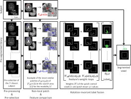
Graphical abstract

Highlights

• •We propose a new multi-channel MS lesion segmentation technique.
• •We adapt for lesion segmentation the non-local means operator to account for multi-contrast and rotation-invariant distance.
• •The proposed method presents highly competitive results compared to state-of-the-art methods.
• •The proposed method provides segmentation quality near inter-rater variability for MS lesion segmentation.
• •Our non-local approach is able to detect structures that vary in size, shape and location such as MS lesions.

1. Introduction

Multiple sclerosis (MS) is a chronic, inflammatory demyelinating disease, which mainly affects the white matter of the central nervous system (CNS) but may also affect the cortex. The disease presents itself with a wide range of clinical manifestations, usually beginning with a relapsing remitting (RRMS) phase. RRMS is characterized by attacks of worsening neurologic function (relapses) that are followed by partial or full recovery (remissions). Relapses are directly related to an underlying inflammation of the CNS, which affects the myelin of the axons and consequently leads to focal “MS lesions”. Because magnetic resonance imaging (MRI) is sensitive to inflammatory and demyelinating changes, it is often used to monitor, identify and quantify MS lesions (Fazekas et al., 1999) that are hyperintense on T2-weighted (T2W) magnetic resonance (MR) images and may become hypointense on T1-weighted (T1W) images. Lesion counts are often used to assess the disease burden and track disease progression as new lesions are related to current disease activity. Both counts are used to assess the efficacy of new therapies (Polman et al., 2011). For the purpose of this article, we focus on lesions commonly called “T2-lesions” (those that are hyperintense on T2W images) and do not consider other sub-types of lesions (i.e., gadolinium enhancing “active lesions”, “black holes” and cortical lesions). MS lesions in MR images are extremely difficult to identify because of inter-subject anatomical variability, lesion location, size, texture and shape. Manual segmentation of MS lesions is still recognized as the gold standard in MS, but it is time consuming and subjects to intra- and inter-expert variability. As an alternative, a multitude of automatic techniques to detect and segment MS lesion has been proposed. However, recent reviews of the literature (Lladó et al., 2012; García-Lorenzo et al., 2013) concluded that automatic MS lesion segmentation is still an unsolved topic. Although promising progress has been made in this field open problems and limitations persist. For example, many techniques are not robust across imaging centers or differing MRI protocols.

Two main categories of classifiers emerge from the literature: unsupervised and supervised. Unsupervised methods do not require manual segmentation of the lesions, but estimate tissue classes or clusters of similar voxels with or without the help of anatomical and MRI knowledge. Many unsupervised techniques were initially developed to classify healthy brain tissues based on MRI intensities into three classes (cerebral spinal fluid (CSF), white matter (WM) and grey matter (GM)). This was done by using fuzzy C-mean and Gaussian mixture models with expectation maximization (EM) (Wells et al., 1996). To detect MS lesions, some groups adapted the Gaussian models by adding an extra class for MS lesions (Kikinis et al., 1999; Souplet et al., 2008) and/or added topological constrains (i.e., the publically available approach LesionTOADS (Shiee et al., 2010)). Others defined lesions as outliers of the mixture model (Van Leemput et al., 2001; Schmidt et al., 2012; Cabezas et al., 2014) or as outliers when comparing the spatial and intensity information of the images to be segmented and library of healthy subjects (Tomas-Fernandez and Warfield, 2011; Tomas-Fernandez and Warfield, 2015). To correct for noise and image artifacts, graph-cut techniques have been used to combine spatial information from the local neighborhoods with the intensity model (García-Lorenzo et al., 2008a; Khayati et al., 2008). Unsupervised techniques suffer from both intensity non-uniformity, in the whole image and in the lesion since this variability in intensities cannot be captured with a single global model. Furthermore, the properties of each image need to be specifically defined which can be difficult when artifacts have properties similar to lesions.

The supervised methods use machine-learning techniques to extract relevant features (e.g. intensity or local gradient) and train automatic classifiers from manual or automatic lesion segmentation datasets. Then, the features of new images to be segmented are compared with the training sets to estimate the lesions. These methods can use different machine-learning approaches including: artificial neural networks (ANN) (Zijdenbos et al., 1994), k-nearest neighbors (K-NN) (Vinitski et al., 1999), decision trees (Kamber et al., 1995), random decision forests (RDF) (Geremia et al., 2011), Bayesian frameworks (Harmouche et al., 2006) and logistic regression (Sweeney et al., 2013). The common limitation of both supervised and unsupervised techniques is their sensitivity to image and lesion variability. However, using the appropriate training set and image features, supervised techniques can potentially identify the MS lesion and compensate for variability in image intensities.

Indeed, it has been shown that many supervised library-based (or multi-atlas) techniques outperform unsupervised model-based segmentation methods (Lao et al., 2008). For example, patch-based methods using non-local means (NLM) for structural segmentation have gained in popularity and shown promising results despite their simplicity (Coupé et al., 2011). Patch-based approaches have been applied to segment a multitude of anatomical structures including the hippocampus (Coupé et al., 2011), brain (Eskildsen et al., 2012), lateral ventricles (Fonov et al., 2012), deep nuclei (Xiao et al., 2014), intracranial cavity (Manjón et al., 2014), brain tissues (Cordier et al., 2013) and other structures of the brain (Rousseau et al., 2011). Although NLM has proven to be useful in segmenting anatomically well-defined structures (e.g. hippocampus and lateral ventricles) they have not yet been applied intensively to MS lesion segmentation.

Given the success of patch-based approaches, we present a library-based NLM approach where voxels with similar surrounding neighborhoods (or patches) are used to estimate the presence of lesions. Contrary to the original patch-based segmentation method (Coupé et al., 2011), we offer two main contributions in order to efficiently address the problem of MS lesion segmentation: i) a rotationally-invariant similarity metric for patch comparison which better captures lesion shape variability and ii) a multi-contrast framework that takes advantage of information derived from T2W and FLAIR images. Indeed, in the context of MS lesion segmentation the dimension, shape, orientation and position of lesions vary greatly (Fig. 3).

Fig. 3.

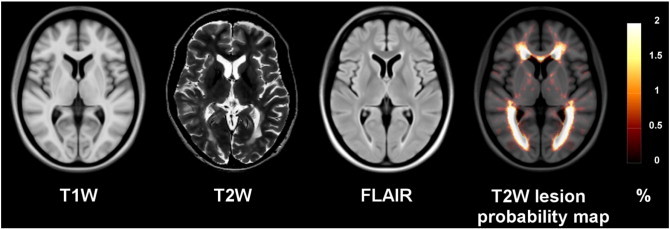
RRMS templates (T1W, T2W, FLAIR) and T2W lesion probability map overlay on the T1W RRMS template.

The sum of squared differences (or L2-norm), which originally used as patch-based distance measure (Buades et al. 2005), is sensitive to the orientation of the patch. While this is good for structure segmentation, this could potentially miss lesion labels (Fig. 1). Similar to the work by Manjón et al. (2012), we replace the L2-norm distance measure with a rotation-invariant distance (RI) where only the intensity of a central voxel and the mean intensity of the patches are considered. Furthermore, the existing NLM segmentation algorithms used a single contrast library (e.g. only T1W images), however, a single image contrast does not hold enough information to separate lesions from healthy tissues. Most lesion segmentation algorithms use T2W and FLAIR MR images, as most MS lesions appear hyperintense on these modalities indicating inflammation or scar tissue. On T1W images, lesions appear hypointense but present a larger intensity variability which might reflect the different sub-types of lesion such as the so-called “black hole” associated with irreversible tissue damage (van Walderveen et al. 1998). Inspired by the work of Coupé et al. (2013), which introduced multi-contrast NLM for image super-resolution and Xiao et al. (2014) for dual-channel NLM segmentation of deep brain structures, we propose an adaptation of the NLM segmentation algorithm to take advantage of multi-contrast images for MS lesion segmentation. This library-based approach captures the potential global and local variability of the anatomy as well as the intensity variability in lesions.

Fig. 1.

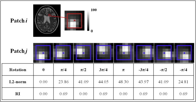
Comparison of L2-norm and RI distance. Different rotations are applied to the extracted patch i (red) to obtain the patches j (blue). The L2-norm and the RI distance metric are then computed between these two patches.

To our knowledge, despite the increasing popularity of patch-based techniques, only a few recent methods have been developed to segment MS lesions. Weiss et al. (2013) presented a supervised segmentation technique using sparse coding with patches from a library of healthy subjects to reconstruct MS patient images. The reconstruction estimates an error map, which detects outliers believed to describe MS lesions. Their method shows promising preliminary results but was not assessed on a large clinical cohort and might not be specific enough to distinguish MS lesions from artifacts when detecting image outliers. The approach by Roy et al. (2014) also uses sparse techniques. In their method, they estimate a weighted average of the most similar patches of a kd-tree using a nearest neighbor search on a library of pre-segmented multi-contrast (T1W and FLAIR) images. While sparse strategies present the advantage of decreasing the dimensionality of the library, kd-tree removes the 3D spatial knowledge of the training images which may hold additional pertinent information that can help identifying MS lesions. Indeed, despite careful pre-processing, the local MS lesion properties in MR images (i.e., intensity, contrast, noise) depend on the local anatomical and/or spatial location of the lesion (Meier and Guttmann, 2003). Thus, by using a 3D volume library, this local information can help capture the spatial layout of different MS lesions. Finally, neither Weiss et al. (2013) nor Roy et al.'s (2014) patch-based approaches for lesion segmentation use rotationally invariant features. As will be demonstrated in Section 3.1.3, this aspect is crucial in the context of MS lesion detection.

We assessed our rotation-invariant multi-contrast non-local means segmentation (RMNMS) approach on 108 RRMS patients from a multi-site clinical study. Our method obtained a Dice similarity measure of 60.1 ± 16.4%, a sensitivity 75.4 ± 15.7% and a precision 55.0 ± 20.1% in cross-validation. Using the parameters established for our initial evaluation, we compared RMNMS to several different state-of-the-art techniques using the datasets from the MS lesion Grand Challenge (MSGC, MICCAI, 2008 (Styner et al., 2008)), on which we obtained very competitive results holding the first rank at the time of the submission.

2. Methods

In the following section we first describe the developed algorithm (Section 2.1), then the dataset (Section 2.2), and lastly our evaluation techniques (Section 2.3).

2.1. The algorithm

Our algorithm adapts the NLM estimator (Section 2.1.1) to account for multi-modal images (Section 2.1.2) and rotation-invariant distance measure of the patches (Section 2.1.3).

2.1.1. The non-local mean approach

2.1.1.1. NLM estimator

The NLM estimator, which takes advantage of image redundancy, was initially proposed by Buades et al. (2005, 2005) for image denoising. The idea of the NLM is to reduce the noise of the image by averaging the voxels that would have a similar intensity in the noise-free image. To achieve the denoising of voxel x(i), the patch P(x(i)) centered on i is compared with all the patches P(x(j)) centered on j of the images in the neighbourhood Ω such that:

$$\widehat{x}\left(i\right)=\frac{{\displaystyle \sum _{j\in \Omega }w\left(i,j\right)l\left(j\right)}}{{\displaystyle {\displaystyle \sum _{j\in \Omega }w\left(i,j\right)}}}\mathit{where}w\left(i,j\right)=e^{-\frac{{‖P\left(x\left(i\right)\right)-P\left(x\left(j_s\right)\right)‖}_2^2}{h^2}}$$ (1)

where the term w(i,j) is a weight based on the similarity of between the patches P(x(i)) and P(x(j)), and is designed to attribute a smaller weight to the greater L2-norm (||.||₂) distance measures. The term h² is a smoothing parameter proportional to the noise variance.

2.1.1.2. NLM segmentation

The NLM approach has been used for structural segmentation (Coupé et al., 2011) by employing a library of atlases with co-registered anatomical images and manually segmented structures to segment those particular structures on new subjects. For NLM segmentation, the weights are estimated between intensities of the subject patch, P(x(i)), and patches from a subject S from library of N pre-segmented subjects, P(x(j_s)), such that:

$$\widehat{x}\left(i\right)=\frac{{\displaystyle \sum _{s=N}{\displaystyle \sum _{j\in \Omega }w\left(i,j_s\right)l\left(j_s\right)}}}{{\displaystyle \sum _{s=N}{\displaystyle \sum _{j\in \Omega }w\left(i,j_s\right)}}}w\left(i,j_s\right)=e^{-\frac{{‖P\left(x\left(i\right)\right)-P\left(x\left(j_s\right)\right)‖}_2^2}{h^2}}$$ (2)

where in this case the h² parameter is set based on the patch minimum distance of the search area (Coupé et al., 2011). Thus, if similar patches are found in the library the minimum distance h² will be low and the weight function will decay quickly such that it is not influenced by other patches.

2.1.2. Multi-contrast NLM segmentation (MNLM)

2.1.2.1. Multi-contrast NLM estimator

In MS, multi-contrast images for manual and automatic segmentation have shown to improve the identification of MS lesions. Inspired by previous work on multi-contrast NLM (MNLM) for denoising (Manjón et al., 2009) and for super-resolution (Coupé et al., 2013), we apply the NLM weighting function to allow for various contrasts (M) such that:

$$w\left(i,j_s\right)=e^{-\left({\displaystyle \sum _M\frac{{‖P_M\left(x\left(i\right)\right)-P_M\left(x\left(j_s\right)\right)‖}_2^2}{{h_M}^2}}\right)}$$ (3)

Here M represents the different MR contrasts commonly used in MS lesion segmentation: T1W, T2W, PDW, or FLAIR for example. It is important to note that the smoothing parameter h_M² is estimated for each considered contrast (i.e., the per contrast minimum distance). Similarly, the L2-norm distance is estimated between patches of the same contrast.

2.1.2.2. Multi-contrast training subject pre-selection

Subjects with similar lesion load and spatial distribution may be more similar with respect to their brain intensity characteristics. Therefore, focusing the weight estimation on the most similar subjects should potentially hold more similar patches, and also presents the advantage of reducing computation. In the context of label fusion segmentation methods, Aljabar et al. (2009) proposed a pre-selection for single contrast images of the most similar structures present in the training library. In our multi-contrast method, we seek the most similar training subjects by measuring the multi-contrast L2-norm (ML2-norm) distance of the subject being segmented and the training subjects across their brain mask region, defined as:

$$\mathrm{ML}2‐\mathrm{norm}={\displaystyle \sum _M{‖I_M\left(x\left(i\right)\right)-L_M\left(x\left(j_s\right)\right)‖}_2}$$ (4)

The N subjects with smallest ML2 distances are selected as they represent the most similar training subjects and thus provide the most similar set of features.

2.1.3. Rotation-invariant multi-contrast non-local mean segmentation (RMNMS)

Previous NLM segmentation implementations have shown convincing results in segmenting anatomically well defined structures (e.g. hippocampus and lateral ventricles (Coupé et al., 2011)). Anatomically, these structures present a relatively small variability of shape, contrast and spatial location making the orientation of the structure to be segmented an important constraint when looking for similar patches in the library. However, this strong advantage for structural segmentation could be a drawback in the context of MS lesion segmentation where no structural, orientation nor spatial location can be assumed. Indeed, Kincses et al. (2011) show that MS lesions can be found almost anywhere in the brain. However, there is spatial predilection for lesions to occupy the peri-ventricular area, the cortico-spinal tract and the optic radiations the lesion distribution probability map as can be shown in Fig. 3. The lesions themselves do not appear to have a constraint on their size, shape or number (as shown in Fig. 3 and Fig. 10 on three MS cases).

Fig. 10.

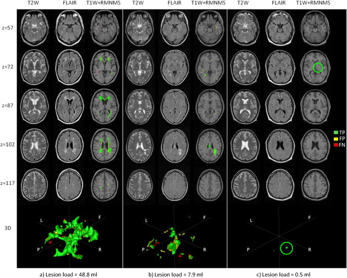
Segmentation results for 3 RRMS cases. a) The largest (48.8 ml), b) median (7.9 ml and c) the smallest (0.5 ml) lesion load of the cohort. The figure shows axial slices (“z” is the z-coordinate in mm in the MNI space) for T2W, FLAIR and T1W combined with the automatic RMNMS segmentation (“T1W + RMNMS”) and 3D rendering of the segmentations (orientation is defined such as F = frontal, P = posterior, R = surgical right and L = surgical left). The overlapping voxels (TP) with the manual segmentation are represented in green, while the false positives (FP) are yellow and the false negatives (FN) are red. The green circle highlights the TP of the unique lesion for subject “c”. The experiment was conducted with a patch radius of 1 voxel, a search area radius of 5 voxels and a pre-selection of 50 training subjects on the 108 RRMS subjects.

In order to increase the ability of the NLM segmentation approach to detect MS lesions, we propose a rotation-invariant distance (RI) metric instead of the L2-norm metric that is used in the multi-contrast NLM framework. Similar to the work of Manjón et al. (2012) on sparseness and self-similarity for MRI denoising, we replaced the L2-norm with a RI distance measure. Therefore, only the intensity of a central voxel (x) and the mean of surrounding patch (µ) are considered:

$$w\left(i,j_s\right)=e^{-\left({\displaystyle \sum _M\frac{{\left(x_M\left(i\right)-x_M\left(j_S\right)\right)}^2+\alpha {\left({\mu }_M\left(i\right)-{\mu }_M\left(j_S\right)\right)}^2}{{h_M}^2}}\right)}$$ (5)

In our experiments, we found that the intensity difference of the central voxels (x_M(i)−x_M(j_S))², was roughly the same as the intensity difference of the patch average (μ_M(i)−μ_M(j_S))², thus we chose α = 1, whereas Manjón et al. (2012) used α = 3. The need for a difference in alpha might be due to our pre-processing and in particular the denoising step, which tends to smooth the neighbouring intensity values surrounding the central voxel. The image denoising step used in our pre-processing (Coupé et al., 2008) is indeed a crucial step as it removes the variability of the central voxel with respect to its neighborhood and therefore allowing a better identification of similar RI features.

In order to be fully invariant to rotation, patches should be spherical, however, we found that cubic patches significantly reduce computational burden while preserving the distance accuracy. A graphical example is provided in Fig. 1, where the distance of a cubic patch containing a lesion and the identical patch subject to different rotations is measured. Indeed, RI provides identical distance measures for different rotations of the same patch, only varying due to sampling and/or interpolation error, while L2-norm varies greatly and favors a larger distance between patches.

Another advantage of the RI distance measure is a reduced computational cost owing to considering only the central voxel and the mean of the patch, rather than all voxels in the patch. To further reduce computational cost we used multithread processing.

2.2. Datasets

As mentioned by García-Lorenzo et al. (2013), simulated datasets, e.g. BrainWeb, enable a good proof of concept validation for image processing methods by providing ground truth images and lesion masks. However, BrainWeb images present multiple limitations: synthetic images are much easier to segment, only one phantom anatomy exists, and BrainWeb lacks contrasts such as FLAIR. Therefore, in this article we focus on two clinical datasets, an RRMS multi-center clinical dataset and the MICCAI (2008) MS Grand Challenge dataset (Styner et al., 2008).

2.2.1. Clinical MS dataset

One clinical multi-center dataset of 108 RRMS patients [age = 42.6 ± 10.7, 72 females] was used to assess the proposed segmentation algorithm. The dataset contains T1W [TE = 9–11 ms, TR = 30–40 ms, flip angle = 30°, in-plane resolution = 0.977 × 0.977 mm², slice thickness = 3 mm], T2W [TE = 66–100 ms, TR = 3550–6610 ms, flip angle = 90°, in-plane resolution = 0.977 × 0.977 mm², slice thickness = 3 mm], PDW [TE = 10–18 ms, TR = 1867–3750 ms, flip angle = 90°, in-plane resolution = 0.977 × 0.977 mm², slice thickness = 3 mm] and FLAIR [TE = 59–94 ms, TR = 7977–9630 ms, TI = 1993–2500 ms, flip angle = 90°, in-plane resolution = 0.977 × 0.977 mm², slice thickness = 3 mm] for all subjects. The MRI data were acquired at 32 sites on 1.5 T scanners from different manufacturers: GE (n = 19), Philips (n = 3) and SIEMENS (n = 10). We do not have access to demographic information for this dataset.

This dataset also contains gold standard MS lesion segmentation labels that were first automatically segmented by a multi-spectral Bayesian classifier (Francis, 2004) with the T1W, T2W and PDW images and manually assessed and corrected by expert raters who underwent extensive training on similar MS patient MRI data. In a previous study (Caramanos et al., 2012), seven raters with similar expertise, corrected the automatically generated lesion labels and were evaluated on a set of 10 MS patients with similar MRI protocols to those used in this study. Thanks to the initial automatic segmentation, this evaluation revealed an excellent inter-rater reliability relative to their trainer's reference segmentations (DSC = 93.5 ± 1.5%) and intra-class correlations (ICC = 99.0 ± 0.5%).

This RRMS cohort presents a large range of lesion loads (0.5–48.8 ml) and lesion counts (1–156 lesions) which are depicted in Fig. 2. In this gold standard delineation protocol, only lesions with at least three connected voxels (or a lesion volume of 0.009 ml) in the 3D volume are kept and considered in our experiments. The MRI data and the expert lesion masks were used to form the template library of our proposed algorithm, which was tested in a leave-one-out fashion.

Fig. 2.

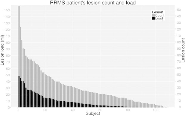
Lesion count and load for each RRMS subject of the clinical cohort. Only lesions with more than three connected voxels (or a lesion volume > 0.009 ml) are considered. The lesion count represents the number of non-connected lesions in grey. The lesion load represents the total volume of lesion (ml) in black. We can note that the lesion load volume is coarsely proportional to the number of lesions.

2.2.2. MS Grand Challenge (MSGC) dataset of MICCAI 2008

Our proposed RMNMS algorithm was further validated using the clinical data provided by the MS lesion segmentation challenge introduced at MICCAI (2008) (Styner et al., 2008). From the MS challenge website1, 20 training MR datasets with ground truth manual lesion segmentations and 23 testing cases were provided from the Boston Children's Hospital (CHB) and the University of North Carolina (UNC). While lesions masks for the 23 testing cases are not available for download, an automated system is available to evaluate the output of a given segmentation algorithm.

We downloaded the co-registered T1W, T2W, FLAIR images for all 43 datasets as well as the ground truth lesion mask images for the 20 training datasets. All images were interpolated at 0.5 mm³ isotropic resolution. We used the MSGC training set as a library to segment the MSGC T2W and FLAIR images.

2.2.3. Pre-processing and training library

All the images from both MS datasets (clinical RRMS and MSGC) were processed using the same pipeline, which does:

• a)NLM image denoising (Coupé et al., 2008).
• b)Intensity non-uniformity correction (N₃) (Sled et al., 1998). Linear intensity normalization of the image histogram to our in-house MS templates that were created with an unbiased template creation algorithm (Fonov et al., 2011) from the 108 T1W images of the RRMS patients (Fig. 3).
• c)Linear registration of each T1W image to our MS template which is in the MNI152 template space (Collins et al., 1994).
• d)Rigid registration of the T2W and FLAIR to the T1W image, followed by resampling onto a 1 × 1 × 1 mm grid in the MNI space. Note that for the purpose of the validation describe here, we used the T1W as the reference image for registration, but other modalities (T2W, FLAIR…) could be chosen if a T1W image is not present or required.
• e)Brain extraction (Eskildsen et al., 2012).

Contrary to some recent patch segmentation approaches (Bai et al., 2013), we did not apply non-linear registration to segment and create the library. This is due to the fact that non-linear registration and interpolation of MS lesions could alter the anatomical and intensity characteristics of MS lesions.

After pre-processing, all of the images and their respective manual segmentation lesion maps are spatially aligned and their intensity distributions are normalized. The denoising step of the pipeline is crucial for the RI distance measure as the central voxel value of a patch is given as much weight as its surrounding patch average. The MS library, used for the segmentation, was built using the output images from the pre-processing stages d, e and f. To double the size of the library and increase the spatial distribution of MS lesions, left–right-mirrored copies of each dataset were added to the library (Fig. 3).

2.3. Evaluation metrics and experiments

In the following section, we describe the general evaluation strategy (Section 2.3.1) and the different metrics (Section 2.3.2) used to assess the proposed segmentation method.

2.3.1. General evaluation strategy

On the clinical RRMS dataset, we performed a leave-one-out cross-validation of the proposed RMNMS method. This leave-one-out cross-validation is achieved by first removing the subject and its respective left–right-mirrored images from the training library, then the multi-modal pre-selection of the N closest subjects are selected and finally the segmentation is performed.

We first evaluated the performance of RMNMS with respect to the search area radius of the patches in the library and the number of pre-selected training subjects (as described in Section 2.1.2).

We also assessed RMNMS using i) different contrast combinations (T1W + FLAIR, T2W + T1W + FLAIR and T2W + FLAIR contrasts), ii) the original L2-norm distance measure version of the NLM segmentation algorithm using T2W + FLAIR contrasts (“T2W + FLAIR NLM”), iii) without the left–right mirror addition to the training library, and iv) the LesionTOADS2 approach proposed by Shiee et al. (2010). LesionTOADS is an iterative atlas based segmentation technique that uses a topological and a statistical atlas within the fuzzy C-means algorithm. As it was originally developed to segment healthy brain tissues (Bazin and Pham, 2008), the algorithm was adapted to use multi-contrast (T1W + FLAIR) and an extra lesion class within the WM class. LesionTOADS was chosen as it is publically available and obtained one the best results during the 2008 MSGC (Styner et al., 2008). Note, that the algorithm was used with its default parameters.

Furthermore, we explored the effect of patients' total lesion-load and lesion-by-lesion detection measures on the RMNMS method.

Two experiments were done using the MSGC dataset. First, our algorithm was validated on the training set using leave-one-out cross-validation. Second, our segmentation results on the testing MSGC dataset were submitted online3 and compared with other published techniques including i) LesionTOADS, ii) Souplet et al. (2008), winner of the MSGC at MICCAI 2008, iii) a recent supervised technique by Geremia et al. (2011) and iv) Tomas-Fernandez et al. (2011), who hold the current best score on the MSGC website before our submission.

For the online MSGC evaluation, we provided the lesion mask in native space after interpolation. The organizers normalized different metric results between 0 and 100, where 100 is a perfect score and 90 is the typical score of an independent rater as described by Styner et al. (2008). The different metrics (volume difference “VolD”, surface distance “SurfD”, true positive rate “TPR” and false positive rate “FPR” (Table 1)) were measured by comparing the automatic segmentation to the manual segmentation of two experts (“CHB” and “UNC”).

Table 1.

Nomenclature of the evaluation metrics. The evaluation metrics are listed in the table below and estimated using the following abbreviations: true positive (TP), lesion-wise true positive (LTP), false positive (FP), lesion-wise false positive (LFP), false negative (FN), lesion-wise false negative (LFN), automatic lesion volume (V_a), manual lesion volume (V_m), $d_a^{am}$ and $d_a^{ma}$ are the Euclidean distances between the automatic (a) and the manual (m) lesion surface voxels, and n_a and n_m are the number of surface voxels for each segmentation.

Name	Abbr.	Equation	Units
Dice similarity measure	DSC	$\frac{2\times TP}{FP+FN+2\times TP}$	%
True positive rate or sensitivity	TPR	$\frac{TP}{TP+FN}$	%
	LTPR	$\frac{LTP}{LTP+LFN}$	%
Positive predictive value or precision	PPV	$\frac{TP}{TP+FP}$	%
	LPPV	$\frac{LTP}{LTP+LFP}$	%
Volume difference	VolD	$\frac{\left|V_a-V_m\right|}{V_m}$	%
False positive rate or fall-out	FPR	$\frac{FP}{FP+TP}$	%
Symmetric surface distance	SurfD	$\frac{1}{\left(n_a+n_m\right)}\left({\displaystyle \sum _{i=1}^{n_a}\left|d_a^{\mathit{am}}\right|}+{\displaystyle \sum _{j=1}^{n_m}\left|d_m^{ma}\right|}\right)$	mm

2.3.2. Evaluation metrics

The quantitative evaluation of our method is carried out using different metrics, summarized in Table 1 as suggested by Styner et al. (2008), and García-Lorenzo et al. (2013).

A high precision (PPV) and sensitivity (TPR) indicate that the automatically segmented lesions correspond well to the manually labeled lesion voxels. A low fall-out (FPR) indicates that the procedure does not identify voxels as lesion when they are not. We measure the absolute volume difference (VolD) of the manual versus the automatic segmentation (0% indicates a perfect lesion volume agreement) and the symmetric surface distance (SurfD) estimates the Euclidean distance between the surfaces of both segmentations at each voxel of their contours (0 mm indicates a perfect match of the surfaces). To estimate the SurfD values, we first estimate the distance transform from the binary segmentation using a 3D-Euclidean metric (Borgefors, 1988) where the surface has a value of 0. Then, we look at the value of the binary segmentation and the corresponding transform distance value to estimate the distance to the surface. Usually, the true positive (TP), false positive (FP) and false negative (FN) rates are voxel-based; however, this measure can also be performed in a lesion-wise manner.

Indeed, in some studies, detecting small lesions is more important than properly identifying their borders. In these comparisons, we use LPPV and LTPR, which are lesion-wise version of the PPV, and TPR metrics where lesion-wise TP (LTP), FP (LFP) and FN (LFN) are measured at each distinct lesion (Table 1). In this case, instead of applying the metrics on a voxel-by-voxel basis, we measure the ability of the method to detect the presence of a lesion. Following the expert manual segmentation protocol, only lesions with at least 3 voxels (or 0.009 ml in the native image space) and an overlap of at least 1 voxel (or 0.003 ml) were considered (Karimaghaloo et al., 2012).

Finally, we assess the behaviour of our method with regard to the patient's lesion load, size and location.

3. Results

The T1W, T2W, and FLAIR RRMS average templates created for the pre-processing stages of our method are presented in Fig. 3 along with the spatial distribution of T2W lesions. While one can appreciate the anatomical definition of the different contrast templates, we can still visually identify the hypo-intense intensity distribution around the lateral ventricles on the T2W and the corresponding hyper-intense intensity on the FLAIR. As expected, the T2W lesion spatial probability distribution is higher is the peri-ventricular region. However, the presence of lesions is diffuse, and our library of MS patients holds enough spatial variation to capture the spatial distribution of lesions.

3.1. Evaluation on the clinical RRMS dataset

3.1.1. Impact of the search area radius

The results for different search area radii on the different metrics (DSC, VolD, TPR, PPV, LTPR and LPPV) are presented in Fig. 4 for RMNMS using T2W + FLAIR. In our experiments, we found that using a patch size of 3 × 3 × 3 provides the best compromise between accuracy and computational burden. With a 3 × 3 × 3 patch (i.e., radius of 1 voxel) and a pre-selection of 50 subjects, the DSC, TPR, PPV, LTPR and LPPV results plateau at their best results with a search area radius of 5 voxels (i.e., 11 × 11 × 11 search area). The volume difference (VolD) results are not as clear but the best results are achieved for any search area radius bigger than 2 voxels. Increasing the search area increases the chance of capturing a patch that is more similar to the considered patch, thus it is not surprising that better results are achieved with bigger search areas. However, increasing the search area needs to balance against computational cost where for instance, increasing the search area from 5 to 6 voxels increases the computational time by 15%. We found a search area radius of 5 voxels to be a good compromise (median results: DSC = 60.1 ± 16.4%, TPR = 75.4 ± 15.7%, PPV = 55.0 ± 20.1%, VolD = 33.5 ± 68.9%, LTPR = 79.8 ± 14.6% and LPPV = 85.7 ± 24.2%) and was chosen for the rest of the evaluation.

Fig. 4.

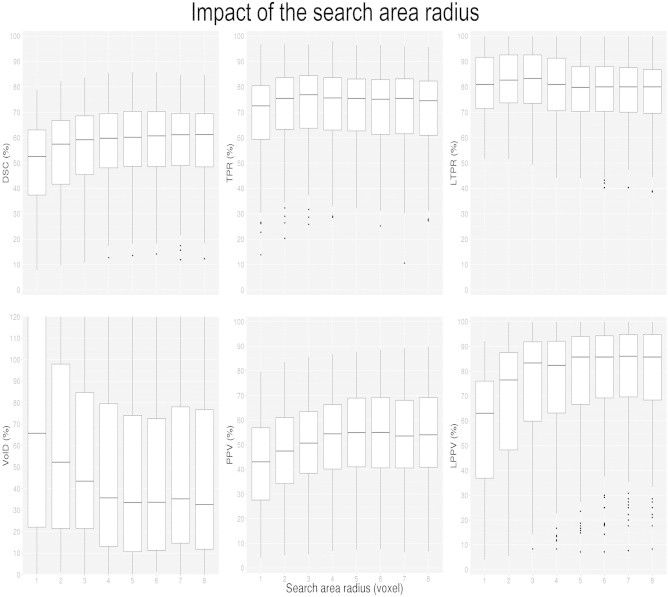
Impact of the search area radius (1–8 voxels) on DSC, VolD, TPR, PPV, LTPR and LPPV distributions. The boxes represent the lower and upper quartile with the median as the central black line. The whiskers extend to the most extreme data point. The experiment was conducted with a patch size radius of 1 voxel, and a pre-selection of 50 subjects.

3.1.2. Impact of the number of pre-selected training subjects

Pre-selecting more subjects from the template library can increase segmentation accuracy. In Fig. 5, the results for the RMNMS method using T2W + FLAIR with different numbers of pre-selected training subjects on the different metrics (DSC, TPR, VolD, PPV, FPR and VolD) are presented. The experiment was performed with a patch radius of 2 (voxels), and a search area radius of 5 voxels while varying the number of pre-selected training subjects from 10 to 80. As expected, increasing the number of subjects in the library improves the quality of the segmentation. Using 50 subjects provides a good comprise between segmentation results and computational cost (median results with 50 pre-selected subjects are the same as in Section 3.1.1, as we used the same parameters) and was chosen for the rest of the evaluation.

Fig. 5.

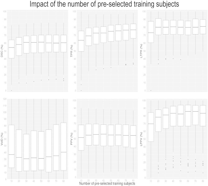
Impact of the number of pre-selected training subjects on DSC, VolD, TPR, PPV, LTPR and LPPV distributions. The experiment was conducted with a patch radius of 1 voxel, and a search area radius of 5 voxels on the 108 RRMS subjects.

3.1.3. Impact of the methods and modalities

Here, we compare RMNMS using T1W + FLAIR, T2W + T1W + FLAIR, T2W + FLAIR with and without the mirrored library images as well as the previous MNLM technique using T2W + FLAIR images, and LesionTOADS using T1W + FLAIR images. RMNMS with T2W + FLAIR was selected as the baseline for comparison and the similarity metric results are summarized in Fig. 6. The main result made evident by Fig. 6 is that RMNMS T2W + FLAIR provides a higher LTPR (79.8 ± 14.6%) than T2W + FLAIR MNLM (67.3 ± 18.6%). Furthermore, T2W + FLAIR RMNMS consistently obtains the highest results (DSC, VolD, PPV, TPR, LTPR and LPPV) when compared to the different modalities used with RMNMS but also when compared with the unsupervised LesionTOADS approach.

Fig. 6.

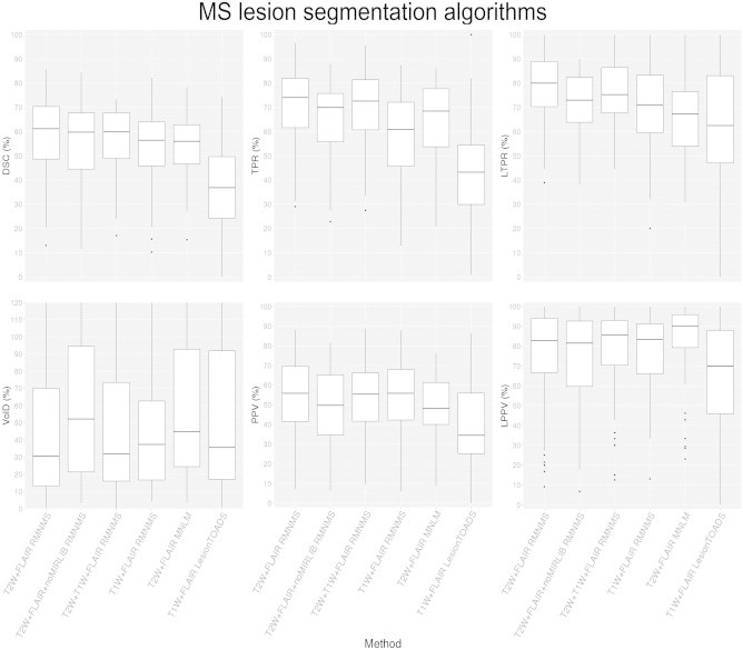
DSC, VolD, TPR, PPV, LTPR and LPPV distributions for different NLM MS lesion segmentation techniques (MNLM and RMNMS), different image modalities (T2W + FLAIR, T1W + FLAIR and T2W + T1W + FLAIR) as well as T2W + FLAIR RMNMS with (T2W + FLAIR RMNMS), without the left–right mirrored of each dataset (T2W + FLAIR+noMIRLIB RMNMS) and T1W + FLAIR LesionTOADS. The experiment was conducted on the 108 RRMS subjects, and for the NLM approaches a patch radius of 1 voxel, and a search area radius of 5 voxels were chosen.

Using T2W + FLAIR images provides overall better segmentation results than the other modality combination and the addition of the left–right mirrored images to the training set improves consistently the segmentation results of T2 + FLAIR RMNMS.

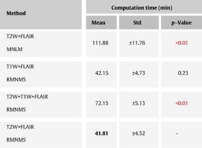
The computational time for RMNMS using 16 threads on an Intel Core i7-950 processor at 3.06 GHz was around 40 min per subject. Our method with these settings is about three times faster (p-value < 0.01) than similar MNLM patch-based methods with the same parameter settings and the computation time for the methods using the entire training set is provided in Table 2.

Table 2.

Computational time results on the RRMS clinical dataset. The proposed method RMNMS, with T2W + FLAIR images, is compared to the original NLM segmentation approach with multi-contrast (MNLM) and a T1W + FLAIR and T2W + T1W + FLAIR version of RMNMS (T1W + FLAIR and T2W + T1W + FLAIR RMNMS). The best measures are shown in bold and the significant difference when comparing with T2W + FLAIR RMNMS is shown in red. The experiment was conducted with a patch radius of 1 voxel, a search area radius of 5 voxels, a pre-selection of 50 subjects for all the methods.

3.1.4. Impact of lesion load and sizes

The segmentation results for patients with different lesion loads are shown in Fig. 7. Subjects with larger lesion loads have better results with lower variability. However, we found that the mean TPR of the method is less affected by the lesion load than the other metrics (i.e., DSC and PPV). Note that DSC is sensitive to object size and smaller DSC is expected for smaller lesions. The linear regression of the manual lesion volume and RMNMS lesion volume shows good correlation with a R² of 0.91, a slope of 1.01 and an intercept of 1.5 ml.

Fig. 7.

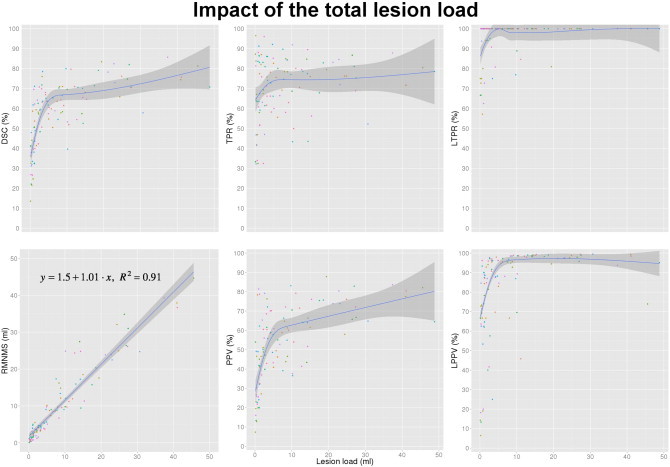
Impact of the lesion load on DSC, manual lesion load linear correlation with RMNMS, TPR, PPV, LTPR and LPPV. The experiment was conducted with a patch radius of 2 voxels, a search area radius of 5 voxels and a pre-selection of 50 training subjects on the 108 RRMS subjects (represented by colored dots on the graph). The blue line represents a non-parametric fitting using a nearest neighbour approach with a locally weighted regression for DSC, TPR and PPV and a linear fitting for the linear regression of the manual lesion load and RMNMS lesion volume. The darker grey shading represents the 95% confidence and for the linear correlation, the slope, the intercept and the residual error (R²) are provided on the graph.

Fig. 8 shows the ability for the RMNMS segmentation to capture the presence of a lesion for different lesion size groups (<0.05, 0.05–0.10 and bigger than 0.10 ml). Sixty percent of all manually segmented lesions are smaller than 0.05 ml and not surprisingly, it is easier to capture the presence of bigger lesions as demonstrated by the LTPR and LPPV (median results: LTPR = 100.0 ± 16.2% and LPPV = 100 ± 17.6%). For the lesions smaller than 0.05 ml, the results are not as good (median results: LTPR = 62.5 ± 20.9% and LPPV = 71.7 ± 26.2%).

Fig. 8.

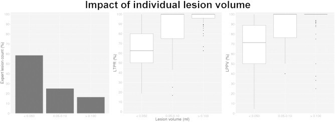
Expert segmentation lesion count, LTPR and LPPV per lesion size groups. The plot on the left shows the manually outline lesion count per each lesion volume group (<0.05, 0.05–0.10, >0.10 ml), averaged across all subjects. The LTPR and LPPV measurement experiments were conducted with a patch radius of 1 voxel, a search area radius of 5 voxels and a pre-selection of 50 training subjects on the 108 RRMS subjects.

3.1.5. Impact of lesion spatial location and examples

In this section we present the RMNMS segmentation results with images to qualitatively describe its spatial behavior.

In Fig. 9, the expert and the automatic RMNMS probability maps of the lesion segmentation show similar frequency and spatial distribution. While the TP and the FP follow the spatial prevalence of the peri-ventricular region, the spatial distribution of the FN is more uniform suggesting non-systematic segmentation errors.

Fig. 9.

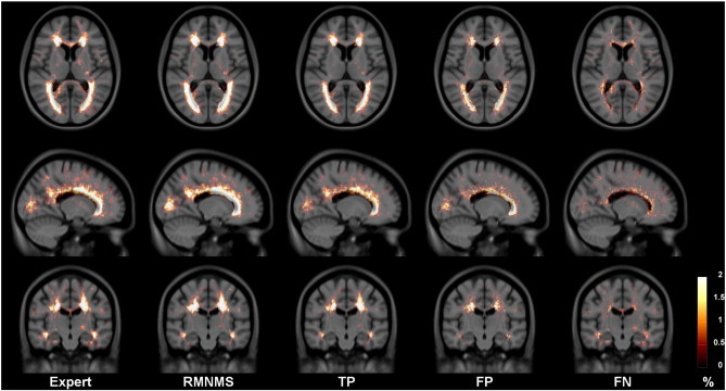
Expert and RMNMS, TP, FP and FN lesion segmentation probability maps for the 108 RRMS patients. All the maps are displayed within the same range and overlaid on the RRMS template T1W.

Fig. 10 shows images of 3 RRMS patients with the highest, median and smallest lesion load with their respective RMNMS segmentation TP, FP and FN. One can appreciate the ability of the method to capture the presence of most of the lesion regardless of the amount and size of the subject's lesions.

3.2. MSGC results

Images from the MSGC were pre-processed like the RRMS dataset. For segmentation, the training library consisted only of the MSGC training dataset. First, we present our leave-one-out cross validation results on the MSGC training set and then we compare our results on the testing set with other methods using an objective web-based system (Styner et al., 2008).

3.2.1. MSGC training dataset

The 20 MSGC training subjects RMNMS segmentations were evaluated in a leave-one-out cross-validation using (20 − 1) × 2 = 38 templates (including the mirrored images). We chose to use a bigger search area radius to compensate for the smaller number of training subject than was available in the RRMS validation. In order to capture the presence of lesions in a greater search area in the library the following parameters were used: patch size radius = 3 and search area radius = 7. It is interesting to note, that the DSC (43.8 ± 16.03) results of RMNMS on this dataset are significantly smaller than for the RRMS dataset (62.3 ± 14.6%). Similar comments can be made for the TPR of 43.9 ± 19.1% and the PPV of 48.7 ± 17.1%.

Given the decreased accuracy of RMNMS with the MSGC dataset we decided to compare the two manual gold standard labels using the same metrics. Comparing the two gold standard manual labels yields a median DSC of 23.7 ± 13.5%, a TPR of 37.1 ± 16.4% and a PPV of 20.2 ± 19.5% confirming the low agreement between the raters.

3.2.2. MSGC testing dataset

The segmentation of the MSGC testing dataset was performed using the whole cohort of training subjects in the template library (20 × 2 = 40) with the same parameters as those used for the training experiment except for the pre-selection number that was set to 40. Our segmentation results were interpolated back to their original space and then uploaded to the MSGC website, where an objective independent automatic evaluation was performed. The MSGC provides a results archive, allowing us to compare the performance of our method with other groups. The results are summarized in Table 3.

Table 3.

VolD, SurfD, TPR and FPR results on the MSGC testing dataset. Our method is compared to 3 methods. The best measures are in bold and the significant differences when comparing with RMNMS are in red for each rater (CHB and UNC).

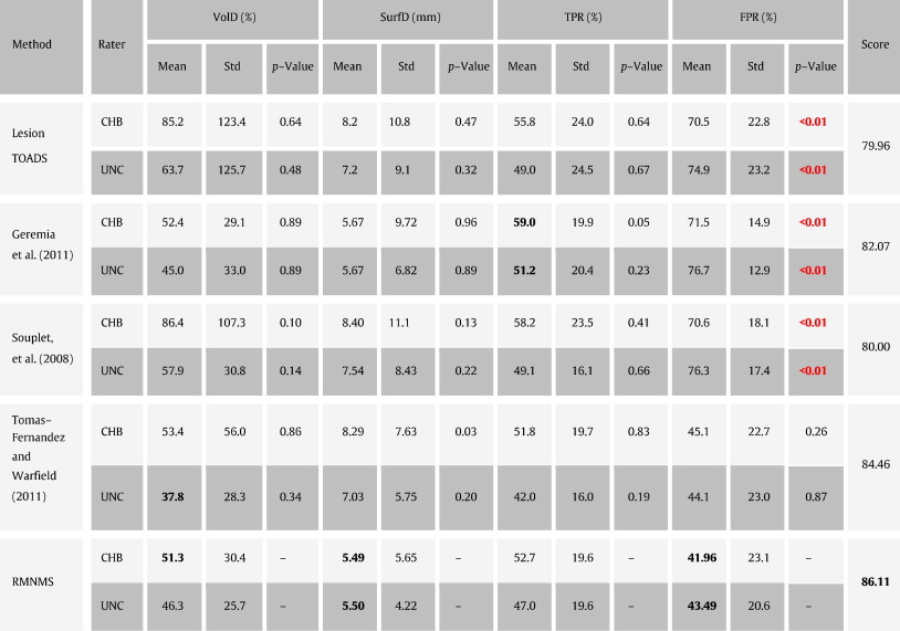
At the time of writing, RMNMS held the best result with an overall average summary score of 86.1 (note that 90 corresponds to a segmentation accuracy reaching human expert inter-rater variability). While RMNMS holds the best results for VolD and SurfD, this advantage is not statistically significant compared to Souplet et al. (2008); Geremia et al. (2011) and LesionTOADS; however RMNMS has a significantly lower FPR when compared to these methods.

4. Discussion

In this article, we proposed a new method to detect MS lesions using a training library containing T2W and FLAIR images along with manual T2W lesion masks. Our adaptation of the increasingly popular NLM segmentation method to MS lesions identification with a new multi-contrast and RI distance measure has proven to be highly competitive in our internal validation and in an independent comparison. On a large clinical dataset of 108 RRMS patient, the best compromise between sensitivity, specificity and computation time using leave-one-out cross-validation was obtained with a patch radius of 1 voxel, a search area radius of 5 voxels and a pre-selection of 50 subjects (median results: DSC = 60.1 ± 16.4%, TPR = 75.4 ± 15.7%, PPV = 55.0 ± 20.1%, VolD = 33.5 ± 68.9%, LTPR = 79.8 ± 14.6% and LPPV = 85.7 ± 24.2%). Given the large RRMS cohort size and variability (e.g. lesion load, age, sex, MRI protocols and scanner brand), these results rank among the best in the MS segmentation literature (Lladó et al., 2012). Furthermore, when compared to the state-of-the-art methods with the publicly available MSGC dataset used during the 2008 MICCAI challenge, the RMNMS yields highly competitive segmentation accuracy (best score, 86.11) and produced segmentations that are comparable to the inter-rater variability.

Our voxel-wise analysis showed promising result with respect to the ability to automatically define the volume and the boundary of the MS lesions. Moreover, our ability to segment MS lesions is relatively independent of the patient's lesion load and lesion location. We also investigated the ability of RMNMS to detect the presence of lesions as lesion-wise measures are often more clinically relevant. For example, lesion count is often used for diagnosis and the evaluation of treatment effect. In this aspect, RMNMS shows a great ability to detect the presence of lesions; it detects almost all lesions bigger than 0.05 ml and 62.5% of lesions smaller than 0.05 ml. Furthermore, due to the ability of RMNMS to explore a large training set cohort with a large search radius, the probability of detecting MS lesions inside anatomical regions is still high within regions of infrequent MS lesions occurrence (i.e., non peri-ventricular lesions).

In both sets of experiments, results were obtained from a multi-center study, which highlights the robustness of our method in the face of inter-site variability. Whereas many methods require at least 3 MRI contrasts (T1W, T2W, PDW or FLAIR) (Souplet et al., 2008; Geremia et al., 2011), and others require even-more contrasts (FLAIR, diffusion tensor imaging fractional anisotropy and mean diffusivity, …) (Morra et al., 2008), we use only two (T2W and FLAIR). This dual-contrast method presents multiple advantages. First, reducing the MRI acquisition time by reducing the number of contrasts can decrease the risk of corruption due to image artifacts, it reduces the financial cost and increases patient comfort. When compared to 3-contrast RMNMS (T2W + T1W + FLAIR), the dual-contrast RMNMS with T2W + FLAIR provides better results with shorter computational time.

NLM segmentation based on a single contrast image shows higher DSC results for the hippocampus (median DSC = 88.4%) (Coupé et al., 2011), brain (DSC = 98.3%) (Eskildsen et al., 2012), lateral ventricles (median DSC = 96.1%) (Fonov et al., 2012) and other structures of the brain (Rousseau et al., 2011). However, DSC is not an optimal similarity metric for small structure segmentation (Rohlfing et al., 2004) and because of spatial scattering, anatomical variability and intensity variations, MS lesion segmentation is a much more complex problem. Indeed, our implementation of the standard NLM segmentation with multi-contrast algorithm (MNLM) only achieves a median LTPR = 67.3%. Where, the multi-contrast RMNMS (T2W + FLAIR) significantly improves the detection of lesions (LTPR = 79.8%) and significantly decreases the computational time. This demonstrates the importance of considering not only the voxel-by-voxel intensity similarity but also the importance of patch-based RI methods for the problem of lesion segmentation. Because of the important reduction in computational time, RMNMS enables the exploration of each training subject with a much wider search radius, which allows for capturing smaller lesions that can even be located in regions where there is low probability of lesion presence in the library. To further increase the presence of similar image in the training library and thus the presence of similar lesions, we used left–right mirrored images and showed the positive impact on the RMNMS segmentation results.

The NLM segmentation technique as applied to the anatomical structures mentioned above requires a smaller set of pre-selected training subjects (20 subjects for hippocampus, lateral ventricles, brain) for optimal results while for MS lesions, RMNMS requires more than 40 training subjects to plateau. This difference can be easily explained by the characteristics of the structure to be segmented where spatial distribution, shape and size of MS lesions are not consistent and thus require a larger number of training subjects to capture this variability. Yet another advantage of the subject training pre-selection in the case of altered images is the selection of the “closest” subjects from the training library. Indeed, despite the presence of artifacts and abnormal intensity non-uniformity in the MSGC dataset (García-Lorenzo et al., 2008b), RMNMS has proven to be highly accurate in part due to the pre-selection of the most representative training subjects.

The comparison of MS lesion segmentation algorithms is a difficult task as described by García-Lorenzo et al. (2013) for multiple reasons: lack of publicly available datasets/methods, differing MRI contrasts, optimal parameters, and inter-rater segmentation variability. Indeed, variation of MS lesion manually defined on the same subject by different experts has been reported to vary greatly by Zijdenbos et al. (2002). The MSGC dataset (Styner et al., 2008) also shows significant inter-rater variability with VolD = 68% and SurfD = 4.85 mm. More importantly, the MSGC training set has an inter-rater reliability of 25% (DSC). One assumes that the MSGC testing set is similar. Despite these criticisms, the organizers of the MSGC are to be congratulated as the MSGC dataset is the first publicly available MS lesion dataset and independent platform for segmentation algorithm validation and comparison. That being said, the MSGC results need to be interpreted carefully with certain limitations in mind. First, the low agreement between the raters should be used as a reference. This can be done by mapping a 25% DSC to a 90% score to represent inter-rater variability when assessing methods. This poor inter-rater agreement may be due to the quality of the images and the presence of multiple artifacts as mentioned by García-Lorenzo et al. (2008a). The high inter-rater variability for the gold standard MSGC labels results in an upper bound on the quality metrics, as it is not possible to simultaneously agree with multiple manual raters that do not agree. For these reasons it is not surprising that RMNMS obtained lower similarity measures on the MSGC than on the clinical RRMS dataset. Second, the MSGC provides pre-processed data (registration, interpolation…), which is not optimal for the different pre-processing steps specific to the different segmentation algorithms. Finally, the online validation metrics are only voxel-wise measures, but the MS segmentation problem cannot be only seen as a voxel-wise or volume difference problem. MS lesion segmentation is also a detection problem especially in the context of clinical studies where a method should capture the presence of all individual lesions. This is not reflected in the global DSC, VolD and SurfD measurements.

Despite these limitations, we compared our approach with state-of-art supervised and unsupervised methods (n > 45) by submitting our segmentation results of the 23 MS test subjects to the MSGC website (Styner et al., 2008). While our RMNMS approach attained the first position at the time of writing with a score of 86.11, this result must be considered with the limitations described above. We feel that our evaluation with the multi-site clinical dataset is much more representative of quality and robustness of the RMNMS technique. We also compared our approach on our RRMS dataset to the popular and publicly available LesionTOADS approach (Shiee et al., 2010). Compared to RMNMS, LesionTOADS is a topology preserving approach guided by probabilistic and topologic atlases. This approach was developed to segment T1W and FLAIR images and as any unsupervised approach it is less flexible to image variability that is not described by the underlying models. These differences could explain the better results obtained by RMNMS on both MS datasets.

Future work will focus on improving segmentation results for smaller lesions, further decrease in the computational time with more advanced patch matching strategy (Ta et al., 2014), investigate the performance and the pre-selection preferences with respect to scanner machine, site, gender and other clinical variables. Finally, we plan to make the RMNMS algorithm available online (http://www.bic.mni.mcgill.ca/RMNMS).

5. Conclusion

We have proposed a new method for segmenting MS lesions. Our method, RMNMS, is a multi-contrast and rotation-invariant distance adaptation of the non-local means operator. RMNMS presents highly competitive results compared to state-of-the-art supervised and unsupervised methods and provides segmentation quality near inter-rater variability for MS lesion segmentation. RMNMS, with multi-contrast and rotation-invariant patch distance, demonstrates that the non-local approach is able to detect structures that vary in size, shape and location such as MS lesions.

References

- Aljabar P., Heckemann R.A., Hammers A., Hajnal J.V., Rueckert D. Multi-atlas based segmentation of brain images: atlas selection and its effect on accuracy. Neuroimage. 2009;46(3):726–738. doi: 10.1016/j.neuroimage.2009.02.018. 19245840 [DOI] [PubMed] [Google Scholar]
- Bai W., Shi W., O'Regan D.P., Tong T., Wang H., Jamil-Copley S., Peters N.S., Rueckert D. A probabilistic patch-based label fusion model for multi-atlas segmentation with registration refinement: application to cardiac MR images. I.E.E.E. Transactions Med. Imaging. 2013;32(7):1302–1315. doi: 10.1109/TMI.2013.2256922. 23568495 [DOI] [PubMed] [Google Scholar]
- Bazin P.-L., Pham D.L. Homeomorphic brain image segmentation with topological and statistical atlases. Med. Image Anal. 2008;12(5):616–625. doi: 10.1016/j.media.2008.06.008. 18640069 [DOI] [PMC free article] [PubMed] [Google Scholar]
- Borgefors G. Hierarchical chamfer matching: a parametric edge matching algorithm. IEEE Trans. Pattern Anal. Machine Intell. 1988;10(6):849–865. [Google Scholar]
- Buades A., Coll B., Morel J.M. CVPR 2005. I.E.E.E. Computer Society Conference. IEEE; 2005. A non-local algorithm for image denoising. Computer vision and pattern recognition. [Google Scholar]
- Cabezas M., Oliver A., Roura E., Freixenet J., Vilanova J.C., Ramió-Torrentà L., Rovira A., Lladó X. Automatic multiple sclerosis lesion detection in brain MRI by FLAIR thresholding. Comput. Methods Programs Biomed. 2014;115(3):147–161. doi: 10.1016/j.cmpb.2014.04.006. 24813718 [DOI] [PubMed] [Google Scholar]
- Caramanos Z., Francis S.J., Narayanan S., Lapierre Y., Arnold D.L. Large, nonplateauing relationship between clinical disability and cerebral white matter lesion load in patients with multiple sclerosis. Arch. Neurol. 2012;69(1):89–95. doi: 10.1001/archneurol.2011.765. 22232348 [DOI] [PubMed] [Google Scholar]
- Collins D.L., Neelin P., Peters T.M., Evans A.C. Automatic 3D intersubject registration of MR volumetric data in standardized Talairach space. J. Comput. Assist. Tomogr. 1994;18(2):192–205. 8126267 [PubMed] [Google Scholar]
- Cordier N., Menze B., Delingette H., Ayache N. Patch-based segmentation of brain tissues. MICCAI Challenge on Multimodal Brain Tumor Segmentation. 2013:6–17. [Google Scholar]
- Coupé P., Manjón J.V., Chamberland M., Descoteaux M., Hiba B. Collaborative patch-based super-resolution for diffusion-weighted images. Neuroimage. 2013;83:245–261. doi: 10.1016/j.neuroimage.2013.06.030. 23791914 [DOI] [PubMed] [Google Scholar]
- Coupé P., Manjón J.V., Fonov V., Pruessner J., Robles M., Collins D.L. Patch-based segmentation using expert priors: application to hippocampus and ventricle segmentation. Neuroimage. 2011;54(2):940–954. doi: 10.1016/j.neuroimage.2010.09.018. 20851199 [DOI] [PubMed] [Google Scholar]
- Coupé P., Yger P., Prima S., Hellier P., Kervrann C., Barillot C. An optimized blockwise nonlocal means denoising filter for 3-D magnetic resonance images. I.E.E.E. Trans. Med. Imaging. 2008;27(4):425–441. doi: 10.1109/TMI.2007.906087. 18390341 [DOI] [PMC free article] [PubMed] [Google Scholar]
- Eskildsen S.F., Coupé P., Fonov V., Manjón J.V., Leung K.K., Guizard N., Wassef S.N., Østergaard L.R., Collins D.L. BEaST: brain extraction based on nonlocal segmentation technique. Neuroimage. 2012;59(3):2362–2373. doi: 10.1016/j.neuroimage.2011.09.012. 21945694 [DOI] [PubMed] [Google Scholar]
- Fazekas F., Barkhof F., Filippi M., Grossman R.I., Li D.K., McDonald W.I., McFarland H.F., Paty D.W., Simon J.H., Wolinsky J.S., Miller D.H. The contribution of magnetic resonance imaging to the diagnosis of multiple sclerosis. Neurology. 1999;53(3):448–456. doi: 10.1212/wnl.53.3.448. 10449103 [DOI] [PubMed] [Google Scholar]
- Fonov V., Coupé P., Styner M., Collins L. Automatic Lateral Ventricle Segmentation in Infant Population with High Risk of Autism. Organization for Human Brain Mapping; Beijing, China: 2012. [Google Scholar]
- Fonov V., Evans A.C., Botteron K., Almli C.R., McKinstry R.C., Collins D.L., Brain, Development Cooperative Group Unbiased average age-appropriate atlases for pediatric studies. Neuroimage. 2011;54(1):313–327. doi: 10.1016/j.neuroimage.2010.07.033. 20656036 [DOI] [PMC free article] [PubMed] [Google Scholar]
- Francis, S.J., Automatic lesion identification in MRI of multiple sclerosis patients (2004). Master's thesis, McGill University, Montreal, Quebec
- García-Lorenzo D., Francis S., Narayanan S., Arnold D.L., Collins D.L. Review of automatic segmentation methods of multiple sclerosis white matter lesions on conventional magnetic resonance imaging. Med. Image Anal. 2013;17(1):1–18. doi: 10.1016/j.media.2012.09.004. 23084503 [DOI] [PubMed] [Google Scholar]
- García-Lorenzo D., Prima S., Collins D.L., Arnold D.L., Morrissey S.P., Barillot C. Combining robust expectation maximization and mean shift algorithms for multiple sclerosis brain segmentation. MICCAI Workshop on Medical Image Analysis on Multiple Sclerosis (Validation and Methodological Issues) (MIAMS'2008) 2008:82–91. [Google Scholar]
- García-Lorenzo D., Prima S., Morrissey S.P., Barillot C. MICCAI Workshop: 3D Segmentation in the Clinic: A Grand Challenge II, MS Lesion Segmentation. 2008. A robust expectation–maximization algorithm for multiple sclerosis lesion segmentation. [Google Scholar]
- Geremia E., Clatz O., Menze B.H., Konukoglu E., Criminisi A., Ayache N. Spatial decision forests for MS lesion segmentation in multi-channel magnetic resonance images. Neuroimage. 2011;57(2):378–390. doi: 10.1016/j.neuroimage.2011.03.080. 21497655 [DOI] [PubMed] [Google Scholar]
- Harmouche R., Collins L., Arnold D., Francis S., Arbel T. Bayesian MS lesion classification modeling regional and local spatial information. I.E.E.E. 18th International Conference on Pattern Recognition, 2006. ICPR 2006. 2006 [Google Scholar]
- Kamber M., Shinghal R., Collins D.L., Francis G.S., Evans A.C. Model-based 3-D segmentation of multiple sclerosis lesions in magnetic resonance brain images. I.E.E.E. Trans. Med. Imaging. 1995;14(3):442–453. doi: 10.1109/42.414608. 18215848 [DOI] [PubMed] [Google Scholar]
- Karimaghaloo Z., Shah M., Francis S.J., Arnold D.L., Collins D.L., Arbel T. Automatic detection of gadolinium-enhancing multiple sclerosis lesions in brain MRI using conditional random fields. I.E.E.E. Trans. Med. Imaging. 2012;31(6):1181–1194. doi: 10.1109/TMI.2012.2186639. 22318484 [DOI] [PubMed] [Google Scholar]
- Khayati R., Vafadust M., Towhidkhah F., Nabavi S.M. A novel method for automatic determination of different stages of multiple sclerosis lesions in brain MR FLAIR images. Comput. Med. Imaging Graphics. 2008;32(2):124–133. doi: 10.1016/j.compmedimag.2007.10.003. [DOI] [PubMed] [Google Scholar]
- Kikinis R., Guttmann C.R., Metcalf D., Wells W.M., Ettinger G.J., Weiner H.L., Jolesz F.A. Quantitative follow-up of patients with multiple sclerosis using MRI: technical aspects. J Magn Reson Imaging. 1999;9(4):519–530. doi: 10.1002/(sici)1522-2586(199904)9:4<519::aid-jmri3>3.0.co;2-m. 10232509 [DOI] [PubMed] [Google Scholar]
- Kincses Z.T., Ropele S., Jenkinson M., Khalil M., Petrovic K., Loitfelder M., Langkammer C., Aspeck E., Wallner-Blazek M., Fuchs S., Jehna M., Schmidt R., Vécsei L., Fazekas F., Enzinger C. Lesion probability mapping to explain clinical deficits and cognitive performance in multiple sclerosis. Mult. Scler. 2011;17(6):681–689. doi: 10.1177/1352458510391342. 21177325 [DOI] [PubMed] [Google Scholar]
- Lao Z., Shen D., Liu D., Jawad A.F., Melhem E.R., Launer L.J., Bryan R.N., Davatzikos C. Computer-assisted segmentation of white matter lesions in 3D MR images using support vector machine. Acad. Radiol. 2008;15(3):300–313. doi: 10.1016/j.acra.2007.10.012. 18280928 [DOI] [PMC free article] [PubMed] [Google Scholar]
- Lladó X., Oliver A., Cabezas M., Freixenet J., Vilanova J.C., Quiles A., Valls L., Ramió-Torrentà L., Rovira À. Segmentation of multiple sclerosis lesions in brain MRI: a review of automated approaches. Inf. Sci. 2012;186(1):164–185. [Google Scholar]
- Manjón J.V., Coupé P., Buades A., Louis Collins D., Robles M. New methods for MRI denoising based on sparseness and self-similarity. Med. Image Anal. 2012;16(1):18–27. doi: 10.1016/j.media.2011.04.003. 21570894 [DOI] [PubMed] [Google Scholar]
- Manjón J.V., Eskildsen S.F., Coupé P., Romero J.E., Collins D.L., Robles M. Nonlocal intracranial cavity extraction. Int. J. Biomed. Imaging. 2014;2014:820205. doi: 10.1155/2014/820205. 25328511 [DOI] [PMC free article] [PubMed] [Google Scholar]
- Manjón J.V., Thacker N.A., Lull J.J., Garcia-Martí G., Martí-Bonmatí L., Robles M. Multicomponent MR image denoising. Int. J. Biomed. Imaging. 2009;2009:756897. doi: 10.1155/2009/756897. 19888431 [DOI] [PMC free article] [PubMed] [Google Scholar]
- Meier D.S., Guttmann C.R. Time-series analysis of MRI intensity patterns in multiple sclerosis. Neuroimage. 2003;20(2):1193–1209. doi: 10.1016/S1053-8119(03)00354-9. 14568488 [DOI] [PubMed] [Google Scholar]
- Morra J., Tu Z., Toga A., Thompson P. MICCAI Workshop: 3D Segmentation in the Clinic: A Grand Challenge II. 2008. Automatic segmentation of MS lesions using a contextual model for the MICCAI grand challenge; pp. 1–7. (MS Lesion Segmentation). [Google Scholar]
- Polman C.H., Reingold S.C., Banwell B., Clanet M., Cohen J.A., Filippi M., Fujihara K., Havrdova E., Hutchinson M., Kappos L., Lublin F.D., Montalban X., O'Connor P., Sandberg-Wollheim M., Thompson A.J., Waubant E., Weinshenker B., Wolinsky J.S. Diagnostic criteria for multiple sclerosis: 2010 revisions to the McDonald criteria. Ann. Neurol. 2011;69(2):292–302. doi: 10.1002/ana.22366. 21387374 [DOI] [PMC free article] [PubMed] [Google Scholar]
- Rohlfing T., Brandt R., Menzel R., Maurer C.R. Evaluation of atlas selection strategies for atlas-based image segmentation with application to confocal microscopy images of bee brains. Neuroimage. 2004;21(4):1428–1442. doi: 10.1016/j.neuroimage.2003.11.010. 15050568 [DOI] [PubMed] [Google Scholar]
- Rousseau F., Habas P.A., Studholme C. A supervised patch-based approach for human brain labeling. I.E.E.E. Trans. Med. Imaging. 2011;30(10):1852–1862. doi: 10.1109/TMI.2011.2156806. 21606021 [DOI] [PMC free article] [PubMed] [Google Scholar]
- Roy S., He Q., Carass A., Jog A., Cuzzocreo J., Reich D., Prince J., Pham D. Example based lesion segmentation. Progress in biomedical optics and imaging. Proc. S.P.I.E. 2014;9034 doi: 10.1117/12.2043917. [DOI] [PMC free article] [PubMed] [Google Scholar]
- Schmidt P., Gaser C., Arsic M., Buck D., Förschler A., Berthele A., Hoshi M., Ilg R., Schmid V.J., Zimmer C., Hemmer B., Mühlau M. An automated tool for detection of FLAIR-hyperintense white-matter lesions in multiple sclerosis. Neuroimage. 2012;59(4):3774–3783. doi: 10.1016/j.neuroimage.2011.11.032. 22119648 [DOI] [PubMed] [Google Scholar]
- Shiee N., Bazin P.-L., Ozturk A., Reich D.S., Calabresi P.A., Pham D.L. A topology-preserving approach to the segmentation of brain images with multiple sclerosis lesions. Neuroimage. 2010;49(2):1524–1535. doi: 10.1016/j.neuroimage.2009.09.005. 19766196 [DOI] [PMC free article] [PubMed] [Google Scholar]
- Sled J.G., Zijdenbos A.P., Evans A.C. A nonparametric method for automatic correction of intensity nonuniformity in MRI data. I.E.E.E. Trans. Med. Imaging. 1998;17(1):87–97. doi: 10.1109/42.668698. 9617910 [DOI] [PubMed] [Google Scholar]
- Souplet J., Lebrun C., Ayache N., Malandain G. MICCAI Workshop: 3D Segmentation in the Clinic: A Grand Challenge II. 2008. An automatic segmentation of T2-FLAIR multiple sclerosis lesions; pp. 1–11. (MS Lesion Segmentation). [Google Scholar]
- Styner M., Lee J., Chin B., Chin M., Commowick O., Tran H., Markovic-Plese S., Jewells V., Warfield S. MICCAI Workshop: 3D Segmentation in the Clinic: A Grand Challenge II. 2008. editorial: 3D segmentation in the clinic: a grand challenge II: MS lesion segmentation; pp. 1–8. (MS Lesion Segmentation). [Google Scholar]
- Sweeney E.M., Shinohara R.T., Shiee N., Mateen F.J., Chudgar A.A., Cuzzocreo J.L., Calabresi P.A., Pham D.L., Reich D.S., Crainiceanu C.M. OASIS is automated statistical inference for segmentation, with applications to multiple sclerosis lesion segmentation in MRI. Neuroimage Clin. 2013;2:402–413. doi: 10.1016/j.nicl.2013.03.002. 24179794 [DOI] [PMC free article] [PubMed] [Google Scholar]
- Ta V.T., Giraud R., Collins D.L., Coupé P. Optimized PatchMatch for near real time and accurate label fusion. Med. Image. Comput. Comput. Assist. Interv. 2014;17(3):105–112. doi: 10.1007/978-3-319-10443-0_14. 25320788 [DOI] [PubMed] [Google Scholar]
- Tomas-Fernandez X., Warfield S.K. A new classifier feature space for an improved multiple sclerosis lesion segmentation. I.E.E.E. International Symposium on Biomedical Imaging: From Nano to Macro. 2011 [Google Scholar]
- Tomas-Fernandez X., Warfield S.K. A model of population and subject (MOPS) intensities with application to multiple sclerosis lesion segmentation. I.E.E.E. Trans. Med. Imaging. 2015 doi: 10.1109/TMI.2015.2393853. [DOI] [PMC free article] [PubMed] [Google Scholar]
- Van Leemput K., Maes F., Vandermeulen D., Colchester A., Suetens P. Automated segmentation of multiple sclerosis lesions by model outlier detection. I. E.E.E. Trans. Med. Imaging. 2001;20(8):677–688. doi: 10.1109/42.938237. 11513020 [DOI] [PubMed] [Google Scholar]
- Van Walderveen M.A., Kamphorst W., Scheltens P., van Waesberghe J.H., Ravid R., Valk J., Polman C.H., Barkhof F. Histopathologic correlate of hypointense lesions on T1-weighted spin-echo MRI in multiple sclerosis. Neurol. 1998;50(5):1282–1288. doi: 10.1212/wnl.50.5.1282. 9595975 [DOI] [PubMed] [Google Scholar]
- Vinitski S., Gonzalez C.F., Knobler R., Andrews D., Iwanaga T., Curtis M. Fast tissue segmentation based on a 4D feature map in characterization of intracranial lesions. J. Magn. Reson. Imaging. 1999;9(6):768–776. doi: 10.1002/(sici)1522-2586(199906)9:6<768::aid-jmri3>3.0.co;2-2. 10373024 [DOI] [PubMed] [Google Scholar]
- Weiss N., Rueckert D., Rao A. Multiple sclerosis lesion segmentation using dictionary learning and sparse coding. Med. Image Comput. Comput. Assist. Interv. 2013;16(1):735–742. doi: 10.1007/978-3-642-40811-3_92. 24505733 [DOI] [PubMed] [Google Scholar]
- Wells W.M., Grimson W.L., Kikinis R., Jolesz F.A. Adaptive segmentation of MRI data. I.E.E.E. Trans. Med. Imaging. 1996;15(4):429–442. doi: 10.1109/42.511747. 18215925 [DOI] [PubMed] [Google Scholar]
- Xiao Y., Fonov V.S., Beriault S., Gerard I., Sadikot A.F., Pike G.B., Collins D.L. Patch-based label fusion segmentation of brainstem structures with dual-contrast MRI for Parkinson's disease. Int. J. Comput. Assist. Radiol. Surg. 2014 doi: 10.1007/s11548-014-1119-4. 25249471 [DOI] [PubMed] [Google Scholar]
- Zijdenbos A.P., Dawant B.M., Margolin R.A., Palmer A.C. Morphometric analysis of white matter lesions in MR images: method and validation. I.E.E.E. Transactions Med. Imaging. 1994;13(4):716–724. doi: 10.1109/42.363096. 18218550 [DOI] [PubMed] [Google Scholar]
- Zijdenbos A.P., Forghani R., Evans A.C. Automatic “pipeline” analysis of 3-D MRI data for clinical trials: application to multiple sclerosis. I.E.E.E. Transactions Med. Imaging. 2002;21(10):1280–1291. doi: 10.1109/TMI.2002.806283. 12585710 [DOI] [PubMed] [Google Scholar]