Design of the Value of Imaging in Enhancing the Wellness of Your Heart (VIEW) Trial and the Impact of Uncertainty on Power

Abstract

Background

Although observational evidence has suggested that the measurement of CAC may improve risk stratification for cardiovascular events and thus help guide the use of lipid-lowering therapy, this contention has not been evaluated within the context of a randomized trial. The Value of Imaging in Enhancing the Wellness of Your Heart (VIEW) trial is proposed as a randomized study in participants at low intermediate risk of future coronary heart disease (CHD) events to evaluate whether coronary artery calcium (CAC) testing leads to improved patient outcomes.

Purpose

To describe the challenges encountered in designing a prototypical screening trial and to examine the impact of uncertainty on power.

Methods

The VIEW trial was designed as an effectiveness clinical trial to examine the benefit of CAC testing to guide therapy on a primary outcome consisting of a composite of non-fatal myocardial infarction, probable or definite angina with revascularization, resuscitated cardiac arrest, non-fatal stroke (not transient ischemic attack (TIA)), CHD death, stroke death, other atherosclerotic death, or other cardiovascular disease (CVD) death. Many critical choices were faced in designing the trial, including: (1) the choice of primary outcome, (2) the choice of therapy, (3) the target population with corresponding ethical issues, (4) specifications of assumptions for sample size calculations, and (5) impact of uncertainty in these assumptions on power/sample size determination.

Results

We have proposed a sample size of 30,000 (800 events) which provides 92.7% power. Alternatively, sample sizes of 20,228 (539 events), 23,138 (617 events) and 27,078 (722 events) provide 80, 85, and 90% power. We have also allowed for uncertainty in our assumptions by computing average power integrated over specified prior distributions. This relaxation of specificity indicates a reduction in power, dropping to 89.9% (95% confidence interval (CI): 89.8 to 89.9) for a sample size of 30,000. Samples sizes of 20,228, 23,138, and 27,078 provide power of 78.0% (77.9 to 78.0), 82.5% (82.5 to 82.6), and 87.2% (87.2 to 87.3), respectively.

Limitations

These power estimates are dependent on form and parameters of the prior distributions.

Conclusions

Despite the pressing need for a randomized trial to evaluate the utility of CAC testing, conduct of such a trial requires recruiting a large patient population, making efficiency of critical importance. The large sample size is primarily due to targeting a study population at relatively low risk of a CVD event. Our calculations also illustrate the importance of formally considering uncertainty in power calculations of large trials as standard power calculations may tend to overestimate power.

1 Background and Rationale for the Study

Cardiovascular disease (CVD) remains the leading cause of death and a major cause of disability in the US population and worldwide, despite advances in the treatment of risk factors for CVD. This public health burden is related, in part, to difficulties in identifying persons at sufficiently high risk of a CVD event as to warrant therapy with lipid-lowering or hypertension medications. Lifestyle changes are recommended at all risk levels. Many persons who experience CVD events are classified as being at low risk by current approaches to risk assessment, such as the Framingham risk score (FRS) for CHD, that are based on risk factor levels measured in clinical settings [1]. Over the past decade, significant interest has developed regarding the role of non-invasive measures of subclinical atherosclerosis in the identification of high risk individuals. A substantial body of observational evidence supports the contention that assessment of coronary artery calcium (CAC) using computed tomography (CT) is very effective in identifying individuals at high and low risk for a CVD event [2, 3, 4, 5, 6]. However, there are no data from randomized trials demonstrating whether a strategy that includes assessment of CAC might lead to different lipid management decisions resulting in better patient outcomes. Several authors have noted the pressing need for definitive data based on randomized trials in order to establish the net public health impact of procedures like CAC testing[7, 8, 9].

Given this need for a randomized trial of CVD risk management strategies incorporating CAC assessments, the primary goal of this paper is to discuss the many challenges faced in designing such an endeavor. Here we present the proposed design of the Value of Imaging in Enhancing the Wellness of Your Heart (VIEW) trial. Although VIEW is not yet funded, we view it as a prototype of a screening trial. Much of our discussion focuses on study scale and efficiency, as VIEW intends to target a population at low-risk of CVD events who would otherwise not be recommended for lipid-lowering therapy. Specifically, we will discuss the definition of the target population along with associated ethical issues, the choice of primary outcome, and the choice of therapy. VIEW also presents a methodological challenge as sample size estimation involves a large number of assumptions, involving varying degrees of uncertainty surrounding each assumption. To evaluate the impact of this uncertainty, we illustrate the use of a combination Bayesian-Frequentist strategy where our uncertainty is translated into a full probability distribution, then calculating the average value of power by integrating over this distribution. Our results indicate that incorporating this uncertainty has important consequences on power/sample size, especially within the context of large-scale trials like VIEW which would involve considerable financial investment.

We begin with a description of the final proposed design for VIEW as many design decisions involve sample size/feasibility considerations. We defer a detailed discussion of these issues until later.

2 Proposed Design for VIEW

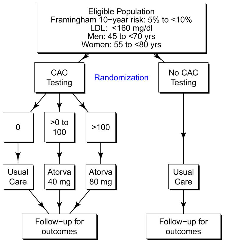
The primary specific aim of VIEW is to test whether a CVD risk management strategy in which lipid-lowering medication use is guided by CAC testing is more effective in preventing CVD events than usual care among persons who are otherwise at relatively low risk of a CHD event. As shown in Figure 1, VIEW is designed as a randomized, controlled trial which proposes to recruit a sample of women (≥ 55 to < 80 years old) and men (≥ 45 to < 70 years old) who are at moderate risk for CHD (5 to < 10% 10-year risk using the FRS CHD equation [1]) with a baseline LDL < 160 mg/dL. Based on data from National Health and Nutrition Examination Survey (NHANES) 2005–2008, we estimate that the targeted study population includes approximately 27 million Americans [10]. Among participants randomized to receive CT testing for CAC, those with a CAC score of 0 would receive no treatment, those with 0 < CAC ≤ 100 would receive 40 mg of atorvastatin daily, and those with CAC > 100 would receive 80 mg of atorvastatin daily. Atorvastatin was chosen because it is one of the most potent statins, has a large market share (currently the drug on which the US spends the most money [11], it had over 40% market share in 2006 [12]) that will likely increase upon becoming generic, and has a better safety profile than does simvastatin [13, 14]. We will also later show that using simvastatin would imply a ≈ 33% larger sample size, making it prohibitively expensive.

Figure 1.

Schematic of the VIEW design.

Participants randomized to no CAC testing will receive usual care, and thus will not be treated as part of the trial protocol. The primary outcome will be time until onset of a new major CVD event defined as a composite of non-fatal myocardial infarction, probable or definite angina with revascularization, resuscitated cardiac arrest, non-fatal stroke (not TIA), CHD death, stroke death, other atherosclerotic death, or other CVD death. This outcome definition is like the all CVD outcome used in the Multi-Ethnic Study of Atherosclerosis (MESA) [15] which also included definite angina not followed by revascularization. We recognize that some untested participants will be treated outside of the trial and that some fraction of people advised to get CAC testing will not get it. The primary analysis will be based on the intention to treat principle. We have assumed a 2.5-year recruitment window with an anticipated 3.5 to 6 years of follow-up. Secondary outcomes will include the components of the primary composite outcome, CVD mortality, an expanded CVD endpoint including revascularizations and heart failure hospitalizations, health-related quality of life, and cost effectiveness.

3 Methods

Sample size determination for VIEW is conceptually straightforward in that it involves a time-to-event outcome with randomization to two study arms. Therefore power/sample size can be calculated as a function of the event rates in each of the study arms (testing for CAC vs. no testing). However, accurately estimating these quantities is complicated by evidence for differential CVD risk by race, FRS, CAC score, and treatment received (dosage of atorvastatin). Therefore the event rates within each study arm are a function of numerous parameters and assumptions, which we now describe in the following sections.

Many of our assumptions are based on data from MESA, which has provided much of the observational evidence concerning the link between CAC and cardiovascular disease [2, 4, 5]. MESA was designed to study the prevalence, risk factors, and progression of subclinical cardiovascular disease in a multiethnic cohort. A detailed description of the study design and methods has been published previously [15]. Briefly, 6814 participants 45 to 84 years of age who identified themselves as white, black, Hispanic, or Chinese were recruited from 6 US communities from 2000 to 2002. All participants were free of clinically apparent cardiovascular disease at the time of recruitment.

In Section 3.1 we will describe how we combine these estimates to calculate power. We will also explore several alternative designs in Section 3.1.4 and perform a sensitivity analysis to illustrate the impact of event rates on power in Section 3.1.5.

Although we were careful to calibrate our power calculations, the large number of assumptions created a concern that our sample size estimates may be sensitive to any inherent misspecification. This was particularly the case for our assumptions concerning the adherence to statin therapy discussed in Section 3.1.1. The large number of parameters also presented a challenge in conducting a typical sensitivity analysis (considering a range of values for each parameter) as this would involve an extremely large number of parameter combinations. To formally incorporate this uncertainty into our estimates of power, we used a hybrid Bayesian-Frequentist approach in Section 3.2, where the uncertainty associated with each parameter is translated into a full probability (prior) distribution [16]. We then compute expected power by averaging with respect to these distributions. The concept of expected power has been described previously by O’Hagan et al. as assurance, or the ‘unconditional probability that a trial will lead to a specific outcome’[17]. This idea has also been suggested by other authors [16, 17, 18, 19], including previous work by the first author within the context of observational studies where the number of individuals with the exposure of interest is not known until after all participants have been recruited [20, 21]. Even though the conceptual idea is simple, this is quite a bit of work in practice, and we have never seen this used in the calculation of power for large randomized controlled trials.

In what follows, we will see that the estimated power using classical techniques for a sample size of 30,000 is 92.7% and, accounting for uncertainty, 89.9% (95% CI: 89.8 to 89.9). We propose 30,000 as our sample size to allow slighly greater margin for error in the misspecification of the parameters assumed.

3.1 Classical Power/Sample Size Determination

3.1.1 Assumptions

FRS scores

Recruitment for VIEW will be largely based on electronic medical records in order to control recruitment costs. This strategy will allow clinic staff to quickly prescreen large numbers of participants at very low cost. However, this screening strategy will likely lead to some individuals being recruited who fall outside the targeted range of FRS risk (5 to < 10%) at baseline. The components of the FRS include gender, age, total cholesterol, high-density lipoprotein cholesterol (HDL), systolic blood pressure (SBP), diabetes, and smoking status [1]. FRS components will be available in the medical record to a varying degree. Gender, age, and SBP will be available on most potential participants, but many will lack a recent lipid panel for total and HDL cholesterol, and smoking status. Absent lipids will preclude recruitment, but smoking status can be confirmed at the time of contact. For individuals lacking smoking status in the record, FRS can be estimated assuming non-smoking and corrected after contact. Lipids may be missing on a significant proportion of potentially eligible persons because screening is recommended only every 5 years for many in the targeted population. We do not plan to repeat blood tests or blood pressure at baseline, or measure these prospectively, to save costs and to make the study more closely resemble usual practice. While we would like to measure both, this would require additional visits that we cannot afford, especially for the 75% of participants who are not receiving medication and who will not be seen in clinic after either the baseline or CT visits.

Because of this approach, we anticipate that some participants will be above and below the target of 5 to < 10% risk as displayed in Table 1. This distribution reflects both errors in the medical records and measurement errors of the risk factors themselves. We denote the probability of being in FRS category i (i = 1, …, 4) as θ_i.

Table 1.

Assumed FRS distribution, denoted as θ_i.

i	FRS	Proportion
1	< 5%	0.0475
2	5 to < 10%	0.9000
3	10 to < 20%	0.0475
4	≥ 20%	0.0050

Race/Ethnicity

Based on NHANES 2005–2008 [10], 79.1% of Americans who meet the eligibility requirements are white, 8.7% are African-American, 7.7% are Hispanic, and 4.5% fall into other race/ethnicity groupings. We plan to over-recruit participants from racial/ethnic minority groups, with an anticipated distribution as shown in Table 2. Because we later use MESA data stratified by race/ethnicity as pilot data, Table 2 is presented in terms of the categories used in MESA. This distribution assumes that 30% of participants will be members of racial/ethnic minority groups (African Americans, Hispanics, Native Americans, and Asians).

Table 2.

Assumed racial/ethnic distribution (using MESA categories).

Race	Proportion
White	0.70
Chinese	0.05
Black	0.15
Hispanic	0.10

Distribution of CAC according to FRS

Eligibility will be based on FRS, with treatment based on the results of CAC assessments. We have used unpublished MESA data in order to calculate “transition matrices” that describe the distribution of CAC according to FRS (similar data have been published [22]). These matrices were calculated separately by race and then a weighted average was calculated using the weights described above resulting in the transition matrix presented in Table 3. These values represent conditional probabilities of a given CAC category for a given FRS range and are denoted as τ_ij. The assumed FRS distribution and the transition matrix results in an assumption that 0.485 of our sample will have a CAC score of 0, 0.299 will be > 0 to ≤ 100 and 0.215 will be > 100. That is, about 0.515 of the group randomized to CAC testing will be expected to be prescribed atorvastatin.

Table 3.

Calculated transition matrix representing the distribution of CAC by FRS, denoted as τ_ij.

i	FRS for CHD	CAC Score
		0	> 0 to ≤ 100	> 100
		j = 1	j = 2	j = 3
1	< 5%	0.540	0.252	0.208
2	5 to < 10%	0.492	0.302	0.206
3	10 to < 20%	0.331	0.298	0.371
4	≥ 20%	0.152	0.261	0.587
	Weighted average	0.485	0.299	0.215

Event Rates

CVD event rates were calculated using unpublished MESA data by race and FRS. As we will recruit primarily based on FRS, we believe that the event rates in MESA should be applicable to VIEW. Assuming an exponential distribution for survival time, the maximum likelihood estimate of the exponential parameter is simply the number of events divided by the total follow-up time. These race- and FRS-specific exponential parameters were then averaged (using the weights above) to calculate the rates presented in Table 4 and are denoted as μ_j.

Table 4.

Assumed event rates by CAC score. The exponential parameters are denoted as μ_j.

j	CAC Score	Exponential Parameter	Proportion/Year	Proportion/10 Years
1	0	0.003053	0.003048	0.030068
2	> 0 to ≤ 100	0.007477	0.007449	0.072042
3	> 100	0.016722	0.016583	0.153986

Loss to Follow-Up

We have assumed loss to follow-up of 0.04/year (exponential parameter of 0.040822).

Adherence to statin therapy

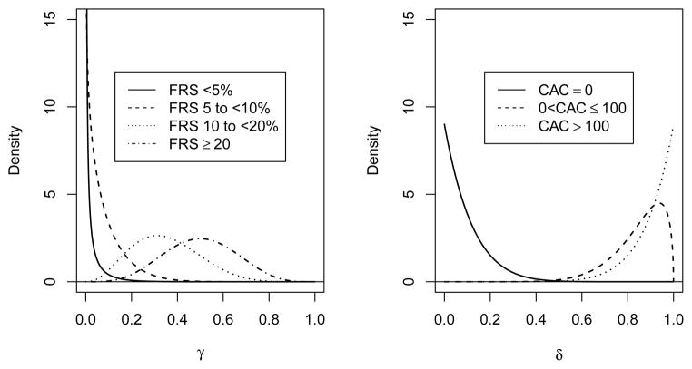
Table 5 presents our assumed adherence profiles. Within the context of the untested group (which will not be prescribed medication by the study), we use the term “adherence” rather generally, as we are aggregating our expectations concerning both adherence to therapy as well as physician behavior in terms of statin prescription. Our adherence estimates for the untested group are based on Kuklina et al [23] and are denoted as γ_ik. For the CAC-tested group, which will be prescribed and provided medication by the study if CAC > 0, adherence estimates are based on the Early Identification of Subclinical Atherosclerosis by Noninvasive Imaging Research (EISNER) Study [24] and are denoted as δ_jk. The adherence profiles incorporate estimates of the proportion of individuals that will take more or less medication than prescribed by the study. This could be because they are prescribed medication by a physician outside the study, because of side effects of atorvastatin (e.g., myalgias or liver function test abnormalities), or for other reasons. These parameters represent the biggest unknowns in our sample size calculation but EISNER suggests that adherence may be quite high in the tested group.

Table 5.

Assumed medication adherence by FRS and CAC. The top half is denoted as γ_ik and the bottom half as δ_jk.

Index	Tested	Risk Level	0 mg	10 mg	20 mg	40 mg	80 mg
			k = 1	k = 2	k = 3	k = 4	k = 5
i = 1	No	FRS < 5%	0.99	0.01	0.00	0.00	0.00
i = 2	No	FRS 5 to < 10%	0.92	0.07	0.01	0.00	0.00
i = 3	No	FRS 10 to < 20%	0.65	0.27	0.05	0.02	0.01
i = 4	No	FRS ≥ 20%	0.50	0.25	0.10	0.10	0.05
j = 1	Yes	CAC = 0	0.90	0.10	0.00	0.00	0.00
j = 2	Yes	0 < CAC ≤ 100	0.15	0.10	0.05	0.65	0.05
j = 3	Yes	CAC > 100	0.10	0.05	0.05	0.05	0.75

We have based our adherence estimates on the EISNER study because it is the largest and most rigorous study of CAC testing in the community. Limitations of prior studies included the lack of a control group, study populations that had a low prevalence of CAC>0, and the lack of direct measurement of risk factors. An important limitation of EISNER is that it was performed in a community with a relatively high socioeconomic status relative to the general population, which may limit its generalizability. However, there are no comparable studies.

Hazard Ratios

The assumed hazard ratios for each dose of atorvastatin are presented in Table 6 and are denoted as κ_k. The Cholesterol Treatment Trialists’ (CTT) Collaboration reported a relative risk (RR) of 0.79 for a 1 mmol/L low-density lipoprotein cholesterol (LDL) reduction [25]. The Anglo-Scandinavian Cardiac Outcomes Trial{Lipid Lowering Arm (ASCOT-LLA) reported a 1.2 mmol/L reduction in LDL for 10 mg atorvastatin vs. placebo [26]. Treating to New Targets (TNT) reported a 0.62 mmol/L LDL reduction for 80 vs. 10 mg atorvastatin [27]. We assumed that the LDL reductions for 20 and 40 mg would be midway between those for 10 and 80 mg.

Table 6.

Assumed hazard ratios by atorvastatin daily dose, denoted as κ_k.

k	Dose	HR
1	0 mg	1
2	10 mg	0.791.2 ≈ 0.75
3	20 mg	0.791.2+0.62/3 ≈0.72
4	40 mg	0.791.2+0.62×2/3 ≈0.68
5	80 mg	0.791.2+0.62 ≈0.65

3.1.2 Combining Assumptions

The final assumption is that each randomized participant has a probability of 0.5 of being assigned to be tested for CAC. The assumed proportion of the sample having any combination of FRS, CAC, and dose received can then be calculated using the probabilities presented in Tables 1, 3, and 5. The proportion of the sample not receiving testing, FRS score i, CAC score j, and dose k would be

$$0.5{\theta }_i{\tau }_{ij}{\gamma }_{ik}$$

and the proportion of the sample receiving testing, FRS score i, CAC score j, and dose k would be

$$0.5{\theta }_i{\tau }_{ij}{\delta }_{jk}.$$

For example, the probability of someone being randomized to not being tested, to having a FRS < 5%, to having a CAC score of 0, and to receiving 0 mg of atorvastatin is 0.5 × 0.0475 × 0.540 × 0.99 = 0.0127 where terms in the product are P(not tested), P(FRS < 5%), P(CAC = 0|FRS < 5%), and P(0 mg dose|not tested and FRS < 5%). This is then calculated for all possible combinations of testing (yes/no), FRS/CAC, and adherence.

Note that the CAC score will only be known for people in the tested group. By randomization, the distribution of CAC scores between tested and untested groups should be comparable. For each combination we assume that the exponential parameter before consideration of the treatment effect is as given in Table 4 which is then multiplied by the appropriate hazard ratio κ_k from Table 6. The average exponential parameter for untested participants is thus

$${\lambda }_0=\sum _{i=1}^4\sum _{j=1}^3\sum _{k=1}^{5}0.5{\theta }_i{\tau }_{ij}{\gamma }_{ik}{\mu }_j{\kappa }_k$$ (1)

and, for tested participants,

$${\lambda }_1=\sum _{i=1}^4\sum _{j=1}^3\sum _{k=1}^{5}0.5{\theta }_i{\tau }_{ij}{\delta }_{jk}{\mu }_j{\kappa }_k.$$ (2)

The hazard ratio can be calculated as λ₁/λ₀.

3.1.3 Sample Size

The sample size can now be calculated using standard techniques. We have used the method presented by Julious [28, Equations 15.8, 15.13, 15.16, and 15.17] which assumes proportional hazards but neither exponential survival nor that the hazards are constant over time. Details of these calculations are presented in Appendix B. We have assumed a two-sided test performed at α = 0.05, a 2.5 year uniform recruitment period, and a total trial length of six years. The exponential parameters from Equations 1 and 2 are 0.007141 and 0.005604 (event rates of 0.712 and 0.559 %/yr) for an overall hazard ratio of 0.785. With these assumptions, we need a sample size of 27,078 (722 events) to have 90% power. Alternatively, sample sizes of 20,228 (539 events), 23,138 (617 events), and 30,000 (800 events) provide 80, 85, and 92.7% power.

3.1.4 Design Alternatives

In the design presented above, we have considered many design alternatives. These include the choices of outcomes, CAC categories to guide therapy, the extent to which individuals outside 5 to 10% FRS are targeted, and the choice of medication. The alternative designs, with one exception, produced larger sample sizes and were thus prohibitively expensive (Table 7). The calculations were similar to those presented above with appropriate modifications to the assumptions. The proposed design (row A) is included for comparison.

Table 7.

Sample sizes required for alternative designs using classical power calculations.

Study Design	Sample Size by Power
	80%	85%	90%
A: Proposed design	20,228	23,138	27,078
B: Hard CVD	42,834	48,998	57,342
C: All CHD	22,026	25,196	29,488
D: Death or any CHD	30,764	35,190	41,184
E: Death or any CVD	26,856	30,722	35,954
F: CAC cutpoints 0/300	21,760	24,892	29,130
G: CAC cutpoints 10/100	23,972	27,420	32,090
H: CAC cutpoints 10/300	25,966	29,702	34,760
I: FRS of 0.04/0.75/0.2/0.01	19,076	21,820	25,536
J: Simvastatin	27,448	31,398	36,744
K: Simvastatin with min 10 mg	27,880	31,892	37,324

Limiting the study to the hard CVD outcome from MESA (by excluding revascularization and resuscitated cardiac arrest) [15], results in a substantial increase in the sample size (row B in Table 7). This estimate uses MESA data for event rates and assumes the same hazard ratios as for the proposed design (see Table 6). The hazard ratios for all CHD were calculated assuming a hazard ratio of 0.78 per 1 mmol/L [29] resulting in a slightly larger sample size (row C). To calculate power for the outcomes of death or any CHD (row D) and death or any CVD (row E) (adding all-cause mortality to the composite outcome), we used the CTT estimate that a 1 mmol/L LDL reduction is associated with a RR of 0.90 for all-cause mortality [25]. We have assumed a RR of 0.84 per mmol/L LDL reduction for the composites of death and either any CHD or CVD which is midway between 0.78 and 0.90. Among MESA participants who experienced either a CHD or death from any cause, 41.4% suffered nonfatal CHD which would result in a weighted RR of 0.85 (= 0.414 × 0.78 + (1 − 0.414) × 0.9) and a slightly larger sample size due to the smaller assumed effect. For CVD the proportion of nonfatal CVD was 0.488 with a weighted RR of 0.85.

We examined CAC cutpoints of 0/300 (row F in Table 7), 10/100 (row G), and 10/300 (row H) all of which resulted in sample sizes larger than the proposed design (0/100, row A). People with FRS scores of 10 to 20% are at greater risk for events than people with scores of 5 to 10% and could reasonably be included in the proposed trial. However, many of these individuals already qualify for statin treatment and we anticipate that the next report of the Adult Treatment Panel (ATP IV) will broaden eligibility beyond that described in ATP III [30], thus increasing the proportion of this risk category who should receive therapy irrespective of their CAC score. We anticipate recruiting from the 10 to 20% risk category for whom ATP IV does not recommend statin therapy (e.g., those with LDL < 100 mg/dL). This would allow us to decrease the sample size slightly: if the proportions within FRS categories are 0.04, 0.75, 0.2, and 0.01 (row I), then the sample sizes can be reduced somewhat from the proposed design.

Finally, we have examined the use of simvastatin rather than atorvastatin because simvastatin is currently the only generic statin. CTT reports that the Heart Protection Study (HPS) resulted in a 1.29 mmol/L reduction in LDL with 40 mg simvastatin as compared with placebo and the Study of the Effectiveness of Additional Reductions in Cholesterol and Homocysteine (SEARCH) demonstrated a reduction of 0.39 mmol/L when comparing 80 mg to 20 mg simvastatin [25]. Using the RR of 0.79 from CTT as previously discussed we can estimate the hazard ratios (HRs) as 1, 0.79^1.29−0.39 ≈ 0.81, 0.79^{1.29−0.39/2} ≈ 0.77, 0.79^1.29 ≈ 0.74, and 0.79^1.29+0.39/2 ≈ 0.70 for 0, 10, 20, 40, and 80 mg of simvastatin. Using the same adherence estimates as for atorvastatin as presented in Table 5 (row J in Table 7) results in sample sizes considerably greater than the proposed design. If anybody who would receive a dose of 10 mg of simvastatin instead receives 20 mg then the sample size is increased yet again (row K). The Food and Drug Administration (FDA) has recently issued a warning against using 80 mg of simvastatin [31] so restricting to a maximum dose of 40 mg would only increase the sample size further.

3.1.5 Effect of Event Rates on Power

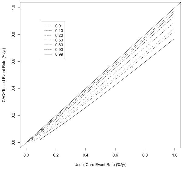
To examine the impact of the event rates on power, we calculated power for a variety of event rates as presented in Table 8 using the assumptions and techniques presented in Section 3.1.3. Power for event rates close to those calculated above is estimated as 0.918. As long as the difference in annual event rates is at least approximately 0.0015, we have power of over 0.9. We have power of over 0.8 as long as the true difference in annual event rates is 0.0013. If the difference is at least 0.0011, we have power of approximately 0.7. Similar information is presented graphically in Figure 2 which is based on a similar figure by Spiegelhalter et al [32].

Table 8.

Power for a sample size of 30,000 for various event rates using the assumptions and techniques described in Section 3.1.3.

CAC-Tested Annual Event Rate	Usual Care Annual Event Rate
	0.0067	0.0069	0.0071	0.0073	0.0075
0.0060	0.349	0.518	0.680	0.812	0.902
0.0058	0.530	0.693	0.823	0.910	0.960
0.0056	0.707	0.835	0.918	0.964	0.986
0.0054	0.846	0.926	0.969	0.988	0.996
0.0052	0.933	0.973	0.990	0.997	0.999

Figure 2.

Contour plot of power by event rates using the assumptions described in Section 3.1.3 for a sample size of 30,000. The proposed design is indicated by the ‘+’. The 45° line is included to guide the eye.

3.2 Uncertainty in Power Calculations

As was mentioned previously, we have considered the calculation of expected power, or assurance, in order to account for the potential impact of uncertainty in our assumptions. Formally, if we let ω (which can vary over Ω) denote our full set of parameters with probability density function f (ω) and π (ω) denote the power for ω, then expected power (EP) can be calculated as

$$\text{EP}=E[\pi ]={\int }_{\omega \in \mathrm{\Omega }}\pi (\omega )f(\omega )d\omega$$ (3)

In Appendix C, we present the probability distributions chosen, as well as their calibration based on data from MESA and the published literature. Calculating the integral in Equation 3 in closed formula is impractical, and so we use Monte Carlo integration to estimate EP as

$$\widehat{\text{EP}}=\frac{1}{N}\sum _{i=1}^N\pi ({\omega }_i)$$

where ω_i is drawn from f (ω) a total of N times [33, Chapter 5]. Likewise, the standard error and confidence interval can be calculated using standard techniques. In what follows, all estimates of EP are based on 1,000,000 Monte Carlo iterations.

With a sample size of 30,000 we estimate expected power to be 89.9% (95% CI: 89.8% to 89.9%)

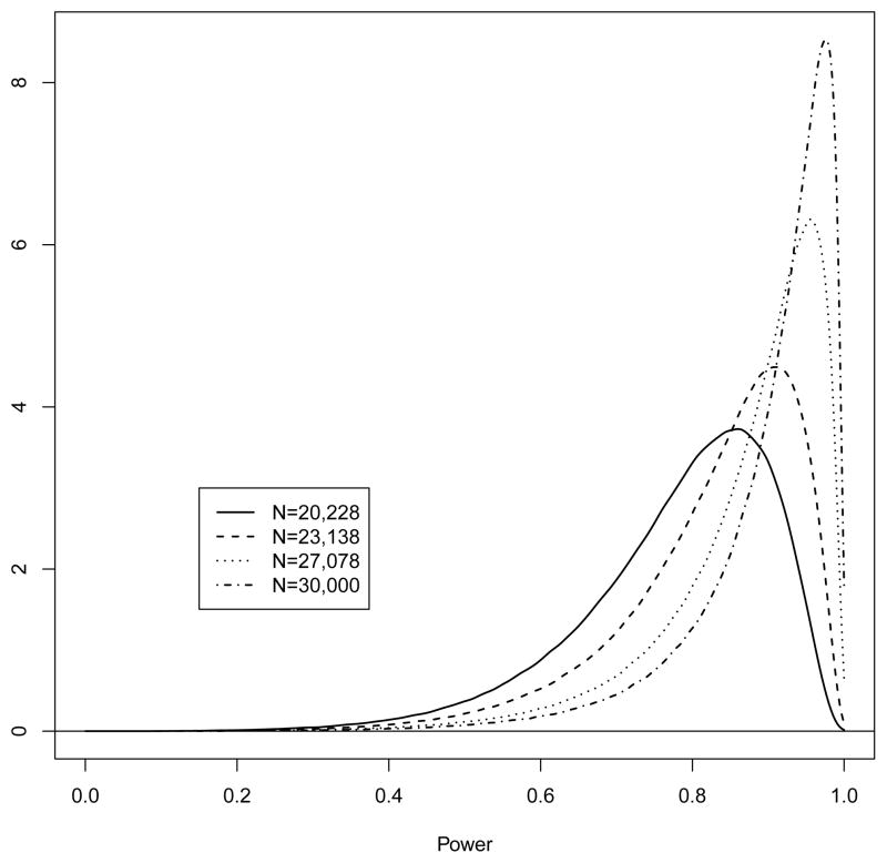
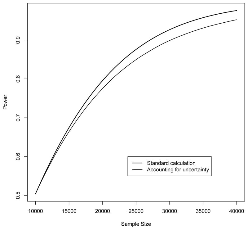
The posterior distribution of EP is presented in Figure 3. The median is 92.9% with a 95% equal tail interval from 62.5% to 99.3%. Samples of 20,228 and 23,138 provide power of 78.0% (77.9 to 78.0) and 82.5% (82.5 to 82.6). Power as a function of sample size can be seen in Figure 4.

Figure 3.

Posterior distribution for power (by simulation). Power is estimated as 78.0, 82.5, 87.2, and 89.9%.

Figure 4.

Power using classical methods and accounting for uncertainty (by simulation) as a function of sample size. The curves were created by calculating power at sample size intervals of 250 and fitting smoothing splines to the resulting data. We used 100,000 simulations for these calculations accounting for uncertainty. Originally we had also included simulation confidence intervals but they were virtually indistinguishable from the estimated mean so were removed.

4 Additional Examples

4.1 Brief Sensitivity Analysis for Prior Distributions

While we did not observe a substantial drop in power after accounting for uncertainty in our assumptions, many of the inputs to our power calculations reflect a sizeable degree of prior data. For example, we used the relative risk reduction associated with a 1 mmol/L reduction in LDL from the CTT (0.79, 95% CI:0.77–0.81), which is based on almost 130,000 participants across 21 randomized trials [25]. If we were considering an intervention which had not been as intensively studied as statin therapy, we believe this would more clearly illustrate the need to routinely estimate the impact of uncertainty on power. For example, we considered a hypothetical scenario where we assumed less precise estimates of the HRs associated with a reduction in LDL (we tripled the standard error for the logarithm of the HR estimate from CTT). In addition, we assumed we had one-third as much information concerning CHD event rates by reducing the hyperparameters of the Gamma prior on each by a factor of 3 (see Appendix C). Assuming a sample size of 30,000 participants, we estimated expected power to be 87.0% (95% CI: 86.9 to 87.0), which now reflects a 5.7% decrease in power compared to the naive estimate of 92.7%.

4.2 Simple Example

To examine the impact of uncertainty on power for a simpler example, we investigated power for a more common design. We assume that the significance level (0.05), study length (6 years), and recruitment period (2.5 years) are fixed and specify priors for the exponential parameter for the event rate (Gamma(40, 10)), for the log of the HR (N(log(0.6), 0.05²)), and for the exponential parameter for the loss rate (the same as presented in Appendix C). The mean exponential parameter for the event rate is 0.4 (annual rate of 0.330), the median HR is 0.6 with the middle 95% of the distribution ranging from 0.544 to 0.662, and the mean annual loss is 0.04. Under these scenarios, 180 people are needed for 80% power and 242 for 90% if we ignore the uncertainty in the event rate, HR, and the loss rate. With 1,000,000 simulations we estimate power as 78.8% (95% CI: 78.8 to 78.8%) for 180 people and as 88.8% (95% CI: 88.8 to 88.8%) for 242 people.

5 Discussion

In the design of this prototype screening trial, we have used a combination of data from other published studies, unpublished MESA data, and recruitment targets to calculate the sample size required for adequate power. Although we believe that these assumptions are reasonable we recognize that every assumption is subject to error. To investigate the impact of these errors on the power of the study, we have defined prior distributions for all parameters and have used simulation to estimate power in the presence of this uncertainty. We are proposing to recruit 30,000 people which we estimate will provide power of 89.9% (95% CI: 89.8 to 89.9). Ignoring uncertainty in the assumptions, we would naively estimate power as 92.7%. While we would have high power with 27,078 participants (naively 90% and 87.2% accounting for uncertainty), we believe that the extra power provided by 30,000 provides protection against unforseen problems and possible misspecification of parameters.

This sample size is as large as it is due primarily to two factors. First, this trial is being conducted only in people at 5 to < 10% Framingham 10-year CHD risk so the expected event rate is low. Second, we will only be treating with atorvastatin about half of those randomized to receive CAC testing and cannot, therefore, expect to see any difference in those who are tested but who have no coronary calcium and are not treated.

We recognize that conducting a randomized trial in 30,000 people will pose numerous challenges, both logistical and financial. To this end, we have made several efforts to simplify the study. First, we plan to work with clinical sites where most of the information required to calculate the FRS is collected as part of routine medical care and is retrievable in electronic medical records. This capability will greatly improve the efficiency of screening and recruitment. Second, we will have very limited data collection at baseline and at follow-up. This will allow us to answer the primary question and have some information about health-related quality of life and cost effective-ness, but will limit our ability to investigate other secondary hypotheses. We anticipate that separately funded ancillary studies will allow some secondary hypotheses to be explored in subsamples. Third, we will use inexpensive means of event ascertainment and follow-up. Participants whose CAC is not measured and those whose CAC is tested but have a zero score (approximately 75% of participants) will not return to the research clinic after the baseline exam. Even the participants randomized to CAC testing and found to be positive, who are then treated with statins will have limited follow-up for laboratory testing and to address adherence issues. Instead of return clinic exams, we will use a combination of telephone, mail, and email contact with the participants to assess for potential events and to measure quality of life. Finally, we will use a centralized strategy to obtain the medical records necessary for adjudication.

A limitation of the current work is that we have not employed a formal elicitation framework in order to quantify the uncertainty implicit to our power calculations (see Garthwaite et al [34]). Even for the quantities heavily based on prior data, we have assumed that their uncertainty can be well-represented by some member of the chosen families of distributions. We have not explicitly evaluated this assumption, in a manner akin to the usual data analysis task of model selection. For quantities which relied on expert opinion, such as the expected adherence to statin therapy, we have similarly assumed that the chosen distributions accurately reflect expert knowledge. Non-parametric elicitation approaches, such as those proposed by Oakley and O’Hagan [35, 36], could therefore be useful in this context. Despite these limitations, the distributions used in our calculations were the result of many hours of discussion between statisticians and content experts, and so we believe they represent reasonable approximations of the current state of knowledge.

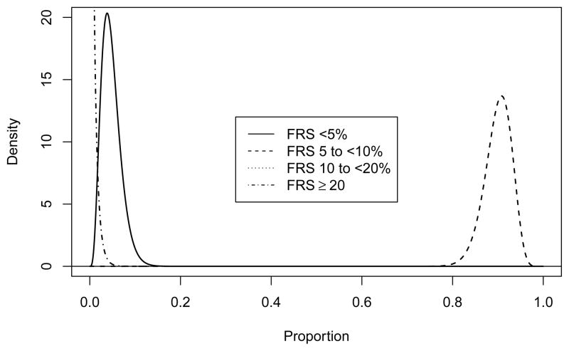
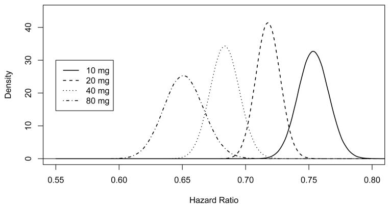
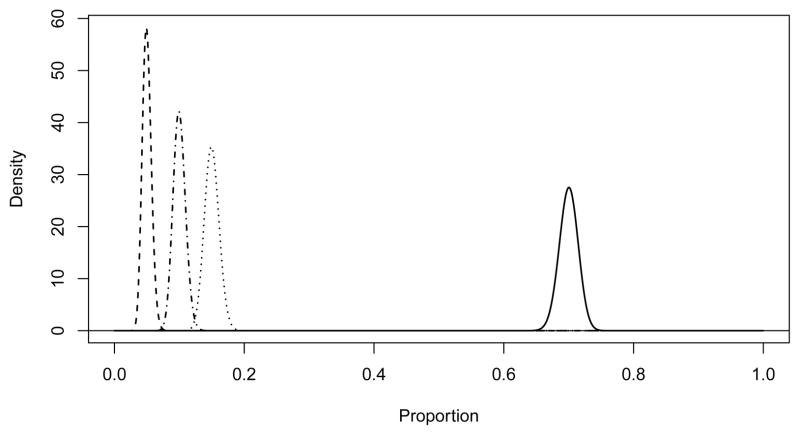
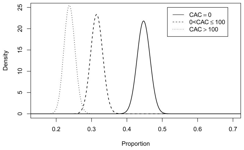
Incorporation of uncertainty by averaging with respect to probability distributions does add a layer of complexity to the process of study design. One of the reviewers raised the concern that this might facilitate confusion with more clinically oriented investigators, possibly obscuring what is actually being assumed. In designing VIEW, we first performed classical power calculations which allowed us to focus on the data necessary for such calculations. Only then did we begin discussions about the uncertainty about these point estimates. Graphical displays of prior distributions such as those described in Appendix C and presented in Figures 5–10 were very helpful in framing the discussions which, while requiring some explanation, were productive and scientifically interesting.

Figure 5.

Prior distribution for FRS. The prior distributions for < 5% and 10 to < 20% are the same.

Figure 10.

Prior distribution for the hazard ratios by daily dose of atorvastatin (by simulation).

Spiegelhalter et al [16] describe conditions under which accounting for uncertainty in the assumptions going into power calculations results in lower estimated power assuming a one-sample Z-test for location, normal data, and a normal prior. As long as the prior is not a point mass and the classical power is greater than 50%, the expected power will be less than the classical power. Using their approach, we observed that power accounting for uncertainty was attenuated towards 50% when classical power was either above or below 50%. We have also seen this in genetic association [20] and other observational studies [21]. In the current context, we have examined this. Sample sizes of 4,260, 9,900, and 17,886, provide classical power of 25, 50, and 75%. Using the same prior distributions used for our proposed sample size of 30,000, we estimated power as 25.4% (95% CI: 25.4 to 25.5%), 50.0% (95% CI: 50.0 to 50.0%), and 73.3% (95% CI: 73.3 to 73.4%). Calculations such as these can also be used for monitoring during the trial much as conditional power [37] is frequently used. Spiegelhalter et al [32] describe this as predictive power.

Although the difference in power ignoring uncertainty (92.7%) and accounting for uncertainty (89.9%) is relatively small, we believe that it represents an important difference that should be considered when designing a study.

A Acronyms

ASCOT-LLA	Anglo-Scandinavian Cardiac Outcomes Trial–Lipid Lowering Arm	14
CAC	coronary artery calcium	2
CI	confidence interval	4
CT	computed tomography	5
CHD	coronary heart disease	2
CTT	Cholesterol Treatment Trialists’	14
CVD	cardiovascular disease	2
EISNER	Early Identification of Subclinical Atherosclerosis by Noninvasive Imaging Research	13
EP	expected power	20
FDA	Food and Drug Administration	19
FRS	Framingham risk score	5
HDL	high-density lipoprotein cholesterol	11
HPS	Heart Protection Study	18
HR	hazard ratio	18
LDL	low-density lipoprotein cholesterol	14
MESA	Multi-Ethnic Study of Atherosclerosis	8
NHANES	National Health and Nutrition Examination Survey	7
RR	relative risk	14
SEARCH	Study of the Effectiveness of Additional Reductions in Cholesterol and Homocysteine	18
SBP	systolic blood pressure	11
TIA	transient ischemic attack	3
TNT	Treating to New Targets	14
VIEW	Value of Imaging in Enhancing the Wellness of Your Heart	1

B Details of Power Calculations

Once we have exponential parameters defining the event rates in the two groups (λ₀ and λ₁), the hazard ratio (HR = λ₁/λ₀), the loss to follow-up rate (ν), the total follow-up time (T), the recruitment period (R), the significance level (α) and the power (1 − β), we can calculate the sample size required. Conversely, we can calculate power based on the sample size and the other parameters.

The number of events needed per group is approximately [28, Equation 15.6]

$$E=\frac{2{(Z_{1-\alpha /2}+Z_{1-\beta })}^2}{{(logHR)}^2}$$ (4)

if we assume exponential survival (and, thus, constant over time). Assuming only that the hazard ratio is constant over time we would need approximately

$$E=\frac{{(HR+1)}^2{(Z_{1-\alpha /2}+Z_{1-\beta })}^2}{2{(HR-1)}^2}$$ (5)

events per group [28, Equation 15.8]. The total number of people is then calculated as [28, Equation 15.3]

$$2E\left[\frac{\left(\frac{f({\lambda }_0)}{{\lambda }_0^2}+\frac{f({\lambda }_1)}{{\lambda }_1^2}\right)}{2}\right]$$

where [28, Equations 15.16 and 15.17]

$$\begin{array}{l}f({\lambda }_0)={\lambda }_0^2{\left[\left(\frac{{\lambda }_0}{\nu +{\lambda }_0}\right)\left(1-\frac{e^{-(T-R)({\lambda }_0+\nu )}-e^{-T({\lambda }_0+\nu )}}{R({\lambda }_0+\nu )}\right)\right]}^{-1}\\ f({\lambda }_1)={\lambda }_1^2{\left[\left(\frac{{\lambda }_1}{\nu +{\lambda }_1}\right)\left(1-\frac{e^{-(T-R)({\lambda }_1+\nu )}-e^{-T({\lambda }_1+\nu )}}{R({\lambda }_1+\nu )}\right)\right]}^{-1}\end{array}$$

account for loss of follow-up and assume a uniform recruitment rate over R.

The sample sizes we calculate using Equation 4 exactly match those from nQuery [38] and come very close to those from SAS [39] which uses slightly different techniques. Using Equation 5 increases the sample size about 1.2% but relaxes the assumption of exponential survival. The calculations presented in this paper use this latter definition.

C Estimation of Expected Power

The prior distributions we chose were either based on MESA data using non-informative hyperpriors or centered at the values described in Section 3.1.1.

FRS Scores

A Dirichlet distribution [40, Chapter 49] was used as the prior for the distribution of FRS scores. The Dirichlet is a multivariate generalization of the beta distribution. We will assume k groups and use the Dirichlet (θ) where θ = (θ₁, …, θ_k). If p ~ Dirichlet (θ) then E [p_i|θ] = θ_i/Θ where $\mathrm{\Theta }={\sum }_{i=1}^k{\theta }_i$.

We are using θ = 100 (θ₁, θ₂, θ₃, θ₄) as the prior distribution where the θ_i are presented in Table 1. The prior distributions for the components of the FRS distribution are presented in Figure 5. The 95% equal tail interval for the proportion of people in the 5 to < 10% group goes from 0.834 to 0.950.

Race

As for FRS, we have used a Dirchlet distribution with parameter

$$\mathit{\theta }=1000(0.70,0.05,0.15,0.10)$$

which has mean equal to the distribution for the study as presented in Table 2. This prior distribution is plotted in Figure 6. The 95% equal tail interval for the proportion of whites goes from 0.671 to 0.728.

Figure 6.

Prior distribution for race. From left to right the distributions are for Chinese, Hispanic, Black, and White.

Transition Matrix

We used unpublished MESA data to calculate the transition matrix for each racial group as described in Section 3. We used a Dirichlet(1,1,1) as a non-informative hyperprior and constructed a Dirichlet prior distribution on the CAC score for each race and FRS combination by adding the observed cell counts to the hyperprior parameters, these are presented in Table 9. To draw a transition matrix, we sampled each row from the appropriate Dirichlet distributions to construct a transition matrix for each race. These were then averaged over the sampled race distribution drawn above as was done previously in Section 3.1.1. The distribution for whites with FRS from 5 to < 10% (the largest group expected in the trial) is presented in Figure 7.

Table 9.

Prior distributions for transition matrices by race.

Race	FRS for CHD	CAC Score
		0	> 0 to ≤ 100	> 100
White	< 5%	266	134	123
White	5 to < 10%	331	233	176
White	10 to < 20%	154	170	245
White	≥ 20%	30	54	168
Chinese	< 5%	79	32	26
Chinese	5 to < 10%	109	75	33
Chinese	10 to < 20%	72	55	39
Chinese	≥ 20%	17	35	27
Black	< 5%	161	67	40
Black	5 to < 10%	303	125	66
Black	10 to < 20%	179	102	84
Black	≥ 20%	40	55	61
Hispanic	< 5%	110	43	22
Hispanic	5 to < 10%	227	99	45
Hispanic	10 to < 20%	161	106	80
Hispanic	≥ 20%	30	51	58

Figure 7.

Prior distribution for CAC scores for whites with FRS from 5 to < 10%.

Event Rates

We have assumed exponential survival. That is, conditional on the parameter λ, the survivial time has density f (x| λ) = λe^−λx. Assuming a hyperprior λ ~ Gamma (α, β), this can be updated using MESA data. If P there are r events and a total follow-up time of T = Σt_i, then it can be easily shown that this results in a Gamma (α + r, β + T) prior distribution for λ. We have chosen to use a non-informative Jeffrey’s prior [41, p53] which reduces to p(λ) ∝ λ⁻¹, which is a Gamma(0, 0).

For each combination of race, FRS, and CAC score we drew from these posterior distributions and averaged these event rates over the FRS and race distributions as described in Section 3.1.1. This results in a vector of exponential parameters for each level of CAC.

Loss to Follow-Up

We assume that the parameter specifying the exponential loss to follow-up is ν ~ Gamma (0.040822 × 400, 1/400) which has mean 0.040822 (0.04/year) and standard deviation of 0.0101. This distribution is plotted in Figure 8. The 95% equal tail interval for this distribution goes from 0.0235 to 0.0629 (annual rates from 0.0232 to 0.0609/year).

Figure 8.

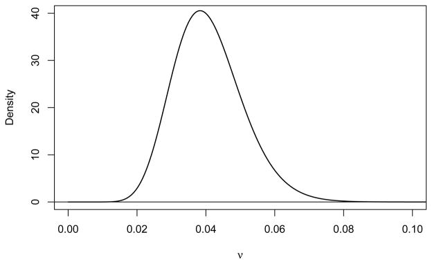
Prior distribution for exponential parameter for loss to follow-up.

Adherence

The prior distributions for adherence as a function of FRS (for those not tested) and as a function of CAC (for those tested) are assumed to be Dirichlet with means 10 times the values presented in Table 5. The prior distributions of the proportions of people receiving some atorvastatin (combining all doses from 10 to 80 mg) are presented in Figure 9.

Figure 9.

Prior distribution for the proportions receiving any atorvastatin by FRS (not tested) and CAC (tested).

Hazard Ratios

Specifying independent prior distributions for each hazard ratio (κ_k) ignores the expectation of a non-increasing rate of major CVD events across increasing doses of atorvastatin. This expectation implies an ordering of the hazard ratios, with

$$({\kappa }_1,\dots ,{\kappa }_k)=\kappa \in S_k=\{1>{\kappa }_0\ge {\kappa }_1\ge \cdots \ge {\kappa }_k\}.$$

We assume the following functional form for the HR for a d mg dose of atorvastatin relative to no drug therapy, HR_d = θ^λ_d where λ_d is the LDL reduction for dose d and θ is the RR per unit reduction in LDL. If we then let η = log (θ), λ₁₀ = δ₁₀, and λ₈₀ = δ₁₀ + δ₈₀, the log HRs for 10 mg and 80 mg of atorvastatin can be defined as

$$\begin{array}{l}{\mathit{LHR}}_{10}=log({HR}_{10})=\eta {\delta }_{10}\\ {\mathit{LHR}}_{80}=log({HR}_{80})=\eta ({\delta }_{10}+{\delta }_{80}).\end{array}$$

CTT reported a relative risk of θ̂ = 0.79 (95% CI:0.77–0.81) for a 1 mmol/L reduction in LDL [25]. This implies η̂ = log(0.79) = −0.2357 with an approximate standard error (SE) of

$$\text{SE}(\widehat{\eta })=\frac{log0.79-log0.77}{{\mathrm{\Phi }}^{-1}(0.975)}=0.0131$$

where Φ⁻¹ (x) is the inverse Gaussian cumulative distribution function.

ASCOT-LLA reported 1-year mean LDL levels of 3.45 (SD = 0.76) for the 4, 384 participants randomized to placebo and 2.25 (SD = 0.69) for the 4, 458 participants randomized to 10 mg of atorvastatin [26]. This implies δ̂₁₀ = 1.20 with an estimated SE of

$$\text{SE}\left(\widehat{{\delta }_{10}}\right)={\left[{\left(\frac{0.69}{\sqrt{4,458}}\right)}^2+{\left(\frac{0.76}{\sqrt{4,384}}\right)}^2\right]}^{1/2}=\mathrm{0.01545.}$$

The TNT trial reported average on-treatment LDL levels of 101 mg/dL and 77 mg/dL (2.612 and 1.991 mmol/L) for 10 mg and 80 mg of atorvastatin respectively [27]. This implies δ̂₈₀ = 0.62064. TNT did not report variability estimates for LDL levels at follow-up, only reporting a SD = 0.46548 mmol/L (18 mg/dL) at baseline for each arm. Assuming comparable variability in LDL levels at follow-up, then

$$\text{SE}\left({\widehat{\delta }}_{80}\right)={\left[{\left(\frac{0.46548}{\sqrt{5,006}}\right)}^2+{\left(\frac{0.46548}{\sqrt{4,995}}\right)}^2\right]}^{1/2}=9.309\times {10}^{-3}.$$

Putting these estimates together, LHR₁₀ = η̂δ̂₁₀ = −0.2829. We can then estimate Var (LHR₁₀) using a first-order delta method approximation assuming independence between η and δ̂₁₀:

$$\begin{array}{l}\text{Var}({\mathit{LHR}}_{10})={\widehat{\delta }}_{10}^2\text{Var}(\widehat{\eta })+{\widehat{\eta }}^2\text{Var}\left({\widehat{\delta }}_{10}\right)\\ =0.0003\\ \text{SE}({\mathit{LHR}}_{10})=\mathrm{0.0161.}\end{array}$$

Assuming that LHR₁₀ ~ N (μ = −0.2829, σ₂ = 0.0161²), this implies a median of e^−0.2829 = 0.7536, with a 95% interval of (0.7300, 0.7780) and 99% interval of (0.7230, 0.7856).

Analogous calculations lead to the following estimates for 80 mg of atorvastatin:

$$\begin{array}{l}\text{Var}({\mathit{LHR}}_{80})={\left({\widehat{\delta }}_{10}+{\widehat{\delta }}_{80}\right)}^2\text{Var}(\widehat{\eta })+{\widehat{\eta }}^2\text{Var}\left({\widehat{\delta }}_{10}\right)+{\widehat{\eta }}^2\text{Var}\left({\widehat{\delta }}_{80}\right)\\ =0.0006\\ \text{SE}({\mathit{LHR}}_{80})=\mathrm{0.0242.}\end{array}$$

Then assuming LHR₈₀ ~ N (−0.4292, 0.0242²), this gives a median of e^−0.4292 = 0.6511 with a 95% interval of (0.6209, 0.6827) and 99% interval of (0.6117, 0.6929). Within the context of the Bayesian averaging for estimating power, at each Monte Carlo iteration we then draw HRs for 10 and 80 mg of atorvastatin using the above defined Gaussian densities. The HRs for 20 and 40 mg are deterministically computed using linear interpolation as

$$\begin{array}{l}log{HR}_{20}^{(i)}=\frac{(log20-log10)log{HR}_{80}^{(i)}+(log80-log20)log{HR}_{10}^{(i)}}{log80-log10}\\ log{HR}_{40}^{(i)}=\frac{(log40-log10)log{HR}_{80}^{(i)}+(log80-log40)log{HR}_{10}^{(i)}}{log80-log10}.\end{array}$$

Table 10 displays summary characteristics of the HR prior distribution based on 1,000,000 iterations. The prior distributions are plotted in Figure 10.

Table 10.

Mean and quantiles of the hazard ratio prior distribution (by simulation).

Dosage	Mean	Q0.005	Q0.025	Q0.5	Q0.975	Q0.995
10 mg	0.754	0.723	0.730	0.754	0.778	0.786
20 mg	0.718	0.702	0.699	0.718	0.737	0.743
40 mg	0.684	0.654	0.661	0.684	0.707	0.714
80 mg	0.651	0.626	0.621	0.651	0.683	0.693

References

- 1.Wilson PWF, D’Agostino RB, Levy D, Belanger AM, Silbershatz H, Kannel WB. Prediction of Coronary Heart Disease Using Risk Factor Categories. Circulation. 1998;97:1837–1847. doi: 10.1161/01.cir.97.18.1837. [DOI] [PubMed] [Google Scholar]
- 2.Greenland P, LaBree L, Azen SP, Doherty TM, Detrano RC. Coronary artery calcium score combined with Framingham score for risk prediction in asymptomatic individuals. JAMA. 2004;291:210–215. doi: 10.1001/jama.291.2.210. [DOI] [PubMed] [Google Scholar]
- 3.Detrano R, Guerci AD, Carr JJ, Bild DE, Burke G, Folsom AR, Liu K, Shea S, Szklo M, Bluemke DA, O’Leary DH, Tracy R, Watson K, Wong ND, Kronmal RA. Coronary calcium as a predictor of coronary events in four racial or ethnic groups. N Engl J Med. 2008;358:1336–1345. doi: 10.1056/NEJMoa072100. [DOI] [PubMed] [Google Scholar]
- 4.Lakoski SG, Greenland P, Wong ND, Schreiner PJ, Herrington DM, Kronmal RA, Liu K, Blumenthal RS. Coronary artery calcium scores and risk for cardiovascular events in women classified as “low risk” based on Framingham risk score: the Multi-Ethnic Study of Atherosclerosis (MESA) Arch Intern Med. 2007;167:2437–2442. doi: 10.1001/archinte.167.22.2437. [DOI] [PubMed] [Google Scholar]
- 5.Polonsky TS, McClelland RL, Jorgensen NW, Bild DE, Burke GL, Guerci AD, Greenland P. Coronary artery calcium score and risk classification for coronary heart disease prediction. JAMA. 2010;16:1610–1616. doi: 10.1001/jama.2010.461. [DOI] [PMC free article] [PubMed] [Google Scholar]
- 6.Möhlenkamp S, Lehmann N, Greenland P, Moebus S, Kälsch H, Schmermund A, Dragano N, Stang A, Siegrist J, Mann K, Jöckel KH, Erbel RL on behalf of the Heinz Nixdorf Recall Study Investigators. Coronary artery calcium score improves cardiovascular risk prediction in persons without indication for statin therapy. Atherosclerosis. 2011;215:229–236. doi: 10.1016/j.atherosclerosis.2010.12.014. [DOI] [PubMed] [Google Scholar]
- 7.Hackam DG, Shojania KG, Spence JD, Alter DA, Beanlands RS, Dresser GK, Goela A, Davies AH, Badano LP, Poldermans D, Boersma E, Njike VY. Influence of Noninvasive Cardiovascular Imaging in Primary Prevention: Systematic Review and Meta-analysis of Randomized Trials. Archives of Internal Medicine. 2011 doi: 10.1001/archinternmed.2011.69. Epub: March 14. [DOI] [PubMed] [Google Scholar]
- 8.Lauer MS. Elements of Danger – The Case of Medical Imaging. New England Journal of Medicine. 2009;361:841–3. doi: 10.1056/NEJMp0904735. [DOI] [PubMed] [Google Scholar]
- 9.Greenland P, Polonsky TS. Time for a policy change for coronary artery calcium testing in asymptomatic people? Journal of the American College of Cardiology. 2011;58(16):1702–4. doi: 10.1016/j.jacc.2011.06.048. [DOI] [PubMed] [Google Scholar]
- 10.Centers for Disease Control and Prevention (CDC). National Center for Health Statistics (NCHS) National Health and Nutrition Examination Survey Questionnaire, Examination Protocol, and Laboratory Protocol. Hyattsville, MD: U.S. Department of Health and Human Services, Centers for Disease Control and Prevention; 2005–2008. [accessed August 7, 2011.]. http://www.cdc.gov/nchs/nhanes.htm. [Google Scholar]
- 11.WebMD. [accessed November 22, 2011.];The 10 Most Prescribed Drugs. http://www.webmd.com/news/20110420/the-10-most-prescribed-drugs.
- 12.Consumer Reports. [accessed November 22, 2011.];The Statin Drugs. http://www.consumerreports.org/health/resources/pdf/best-buy-drugs/Statins-RxTrend-FINAL-Feb2007.pdf.
- 13.Egan A, Colman E. Weighing the Benefits of High-Dose Simvastatin against the Risk of Myopathy. New England Journal of Medicine. 2011;365:285–287. doi: 10.1056/NEJMp1106689. [DOI] [PubMed] [Google Scholar]
- 14.United States Food and Drug Administration. [accessed August 15, 2011.]; http://www.fda.gov/ForConsumers/ConsumerUpdates/ucm257884.htm.
- 15.Bild DE, Bluemke DA, Burke GL, et al. Multi-Ethnic Study of Atherosclerosis: Objectives and Design. American Journal of Epidemiology. 2002;156:871–881. doi: 10.1093/aje/kwf113. [DOI] [PubMed] [Google Scholar]
- 16.Spiegelhalter DJ, Abrams KR, Myles JP. Bayesian Approaches to Clinical Trials and Health-Care Evaluation. Wiley; Chicester: 2004. pp. 193–194. [Google Scholar]
- 17.O’Hagan A, Stevens JW, Campbell MJ. Assurance in clinical trial design. Pharmaceutical Statistics. 2005;4:187–201. doi: 10.1002/pst.175. [DOI] [Google Scholar]
- 18.Fay MP, Halloran ME, Follmann DA. Accounting for variability in sample size estimation with applications to nonadherence and estimation of variance and effect size. Biometrics. 2007;63:465–474. doi: 10.1111/j.1541-0420.2006.00703.x. 10.1111/j.1541-0420.2006.00703.x. 6. [DOI] [PubMed] [Google Scholar]
- 19.Julious SA, Owen RJ. Sample size calculations for clinical studies allowing for uncertainty about the variance. Pharmaceutical Statistics. 2006;5:29–37. doi: 10.1002/pst.197. [DOI] [PubMed] [Google Scholar]
- 20.Ambrosius WT, Lange EM, Langefeld CD. Power for Genetic Association Studies with Random Allele Frequencies and Genotype Distributions. American Journal of Human Genetics. 2004;74:683–693. doi: 10.1086/383282. [DOI] [PMC free article] [PubMed] [Google Scholar]
- 21.Ambrosius WT, Mahnken JD. Power for studies with random group sizes. Statistics in Medicine. 2010;29:1137–1144. doi: 10.1002/sim.3873. [DOI] [PMC free article] [PubMed] [Google Scholar]
- 22.Okwuosa TM, Greenland P, Ning H, Liu K, Bild DE, Burke GL, Eng J, Lloyd-Jones DM. Distribution of Coronary Artery Calcium Scores by Framingham 10-Year Risk Strata in the MESA (Multi-Ethnic Study of Atherosclerosis) Journal of the American College of Cardiology. 2011;57 (18):1838–45. doi: 10.1016/j.jacc.2010.11.053. [DOI] [PMC free article] [PubMed] [Google Scholar]
- 23.Kuklina EV, Yoon PW, Keenan NL. Trends in High Levels of Low-Density Lipoprotein Cholesterol in the United States, 1999–2006. JAMA. 2009;302:2104–2110. doi: 10.1001/jama.2009.1672. [DOI] [PubMed] [Google Scholar]
- 24.Rozanski A, Gransar H, Shaw LJ, et al. Impact of Coronary Artery Calcium Scanning on Coronary Risk Factors and Downstream Testing: The EISNER (Early Identification of Subclinical Atherosclerosis by Noninvasive Imaging Research) Prospective Randomized Trial. J Amer College of Cardiology. 2011;57:1622–1632. doi: 10.1016/j.jacc.2011.01.019. [DOI] [PMC free article] [PubMed] [Google Scholar]
- 25.Cholesterol Treatment Trialists’ (CTT) Collaboration. Efficacy and safety of more intensive lowering of LDL cholesterol: a meta-analysis of data from 170 000 participants in 26 randomized Trials. Lancet. 2010;376:1670–1681. doi: 10.1016/S0140-6736(10)61350-5. [DOI] [PMC free article] [PubMed] [Google Scholar]
- 26.Server PS, Dahlöf B, Poulter NR, et al. for the ASCOT investigators. Prevention of coronary and stroke events with atorvastatin in hypertensive patients who have average or lower-than-average cholesterol concentrations, in the Anglo-Scandinavian Cardiac Outcomes Trial–Lipid Lowering Arm (ASCOT-LLA): a multicentre randomised controlled trial. Lancet. 2003;361:1149–1158. doi: 10.1016/S0140-6736(03)12948-0. [DOI] [PubMed] [Google Scholar]
- 27.LaRosa JC, Grundy SM, Waters DD, et al. for the Treating to New Targets (TNT) Investigators. Intensive Lipid Lowering with Atorvastatin in Patients with Stable Coronary Disease. N Engl J Med. 2005;352:1425–1435. doi: 10.1056/NEJMoa050461. [DOI] [PubMed] [Google Scholar]
- 28.Julious SA. Sample Sizes for Clinical Trials. Chapman & Hall/CRC; Boca Raton, FL: 2010. [Google Scholar]
- 29.Delahoy PJ, Magliano DJ, Webb K, Grobler M, Liew D. The Relationship Between Reduction in Low-Density Lipoprotein Cholesterol by Statins and Reduction in Risk of Cardiovascular Outcomes: An Updated Meta-Analysis. Clinical Therapeutics. 2009;31:236–244. doi: 10.1016/j.clinthera.2009.02.017. [DOI] [PubMed] [Google Scholar]
- 30.Expert Panel on Detection, Evaluation, and Treatment of High Blood Cholesterol in Adults. Executive Summary of the Third Report of the National Cholesterol Education Program (NCEP) Expert Panel on Detection, Evaluation, and Treatment of High Blood Cholesterol in Adults (Adult Treatment Panel III) JAMA. 2001;285:2486–2497. doi: 10.1001/jama.285.19.2486. [DOI] [PubMed] [Google Scholar]
- 31.Food and Drug Administration. [accessed August 7, 2011.]; http://www.fda.gov/Drugs/DrugSafety/ucm256581.htm.
- 32.Spiegelhalter DJ, Freedman LS, Blackburn PR. Monitoring Clinical Trials: Conditional or Predictive Power? Controlled Clinical Trials. 1986;7:8–17. doi: 10.1016/0197-2456(86)90003-6. [DOI] [PubMed] [Google Scholar]
- 33.Hammersley JM, Handscomb DC. Monte Carlo Methods. Methuen & Co. Ltd; London: 1964. [Google Scholar]
- 34.Garthwaite PH, Kadane JB, O’Hagan A. Statistical Methods for Eliciting Probability Distributions. J of the American Statistical Association. 2005;100 (470):680–700. [Google Scholar]
- 35.Oakley JE, O’Hagan A. Uncertainty in prior elicitations: a nonparametric approach. Biometrika. 2007;94 (2):427–441. [Google Scholar]
- 36. [accessed August 8, 2011.];SHeffeld ELicitation Framework (SHELF) http://www.tonyohagan.co.uk/shelf/
- 37.Proschan MA, Lan KKG, Wittes JT. Statistical Monitoring of Clinical Trials: A Unified Approach. New York: Springer; 2006. [Google Scholar]
- 38.Elashoff JD. nQuery Advisor Version 7.0 User’s Guide. Los Angeles, CA: 2007. [Google Scholar]
- 39.SAS Institute, Inc. SAS/STAT 9.2 User’s Guide. SAS Institute; Cary, NC: 2008. pp. 4809–5039. [Google Scholar]
- 40.Kotz S, Balakrishnan N, Johnson NL. Continuous Multivariate Distributions, Volume 1: Models and Applications. 2. Wiley; New York: 2000. [Google Scholar]
- 41.Gelman A, Carlin JB, Stern HS, Rubin DB. Bayesian Data Analysis. Chapman & Hall/CRC; Boca Raton: 1995. [Google Scholar]