Generalized T² Test for Genome Association Studies

Abstract

Recent progress in the development of single-nucleotide polymorphism (SNP) maps within genes and across the genome provides a valuable tool for fine-mapping and has led to the suggestion of genomewide association studies to search for susceptibility loci for complex traits. Test statistics for genome association studies that consider a single marker at a time, ignoring the linkage disequilibrium between markers, are inefficient. In this study, we present a generalized T² statistic for association studies of complex traits, which can utilize multiple SNP markers simultaneously and considers the effects of multiple disease-susceptibility loci. This generalized T² statistic is a corollary to that originally developed for multivariate analysis and has a close relationship to discriminant analysis and common measure of genetic distance. We evaluate the power of the generalized T² statistic and show that power to be greater than or equal to those of the traditional χ² test of association and a similar haplotype-test statistic. Finally, examples are given to evaluate the performance of the proposed T² statistic for association studies using simulated and real data.

Introduction

Lack of tangible success of genetic linkage analyses for mapping of multifactorial trait loci with small-to-moderate effects, coupled with progress in the development of detailed SNP maps of the human genome (Gray et al. 2000), has led to the suggestion of population-based genomewide association studies (Risch and Merikangas 1996) that are based on linkage disequilibrium (LD). Traditional population-based association studies compare marker-allele frequencies between cases and control subjects, separately for each marker. However, when a collection of SNP markers is available, using only a single marker each time and ignoring the nonindependence among markers are inefficient. In addition, it is well known that complex diseases are influenced by multiple genes, requiring the development of statistical methods for evaluation of several trait loci collectively (Longmate 2001). Recently, discriminant analysis (Li et al. 2000), logistic regression (Czika et al. 2000), decision trees (Zhang and Bonney 2000), and neural networks (Bhat et al. 1999; Sherriff and Ott 2001) have been applied to genetic association studies using multiple marker loci. However, such methods provide only classification accuracy as a measure of significance—rather than P values, which are widely used to show significant evidence of association in the traditional context. Therefore, there is a need to describe the relationship between classification methods and traditional statistical testing.

In this article, we present, for population-based association studies of complex diseases, a generalized T² test that simultaneously utilizes multiple SNP markers. The power of the generalized T² statistic for the detection of a disease locus (or loci) will be evaluated, as will be comparability of the genotype T² and haplotype T² statistics.

In addition, we formulate the problem of identification of SNP markers or a combination of SNP markers, which make the largest contribution to disease risk, as a combinatorial optimization problem, and we develop efficient search algorithms. Finally, examples will be given to illustrate the applications of the proposed T² statistic to association studies.

Test Statistic

Consider a design in which n_A cases from an affected population and control subjects from a comparable unaffected population are sampled. Suppose that there are J markers that have been typed in the sample of cases and control subjects. The jth marker has alleles B_j and b_j, with population frequencies P_Bj and P_bj, respectively. Define an indicator variable for the genotype of the jth marker for the ith individual from the affected population:

Similarly, we define an indicator variable, Y_ij, for an individual from the unaffected population. Let

The pooled-sample variance-covariance matrix of the indicator variables for the marker genotypes is defined as

Hotelling’s (1931) T² statistic is then defined as

Under the null hypothesis that LD between any marker being tested and a disease locus does not exist, the covariance matrix of the indicator variables for the marker genotypes of the individuals from the affected population, Σ_A=Cov(X_i,X_i), and the covariance matrix of indicator variables for the marker genotypes of the individuals from the unaffected population, , are equal. Therefore, when the sample size is large enough to allow asymptotic theory to apply, under the null hypothesis,

is asymptotically distributed as a central F distribution with J and degrees of freedom. Under the alternative hypothesis that there is at least one marker showing LD with a disease locus, the covariance matrices Σ_A and are no longer equal and

is not asymptotically distributed as a noncentral F distribution. In this case, it can be shown that T² is asymptotically distributed as a χ²_(J) distribution.

Power Evaluation

Noncentrality Parameter

To evaluate power, we need to calculate the noncentrality parameter of the χ²_(J) distribution of the T² statistic under the alternative hypothesis. We begin by computing the allele frequencies in the affected and unaffected populations. Consider a disease locus with alleles D and d. The alleles D and d have population frequencies P_D and P_d, respectively. Let f_DD, f_Dd, and f_dd be the penetrance of the genotypes DD, Dd, and dd, respectively. Let P_A denote the prevalence of the disease in the population. Then, P_A is given by

Let P_B(A) and be the frequencies of marker allele B in the affected and unaffected populations, respectively. Let P_BD, P_Bd, P_bD and P_bd be the frequencies of haplotypes BD, Bd, bD, and bd, respectively. The frequency P_B(A) is given by

Similarly, we have

where , , and .

Consider the jth marker and the j^′th marker. Let P_BjBj^′(A) and be the frequencies of haplotype B_jB_j^′ in the affected and unaffected populations, respectively. If Hardy-Weinberg equilibrium is assumed, then it is easy to see that (see Appendix A)

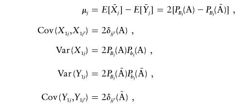where

Define

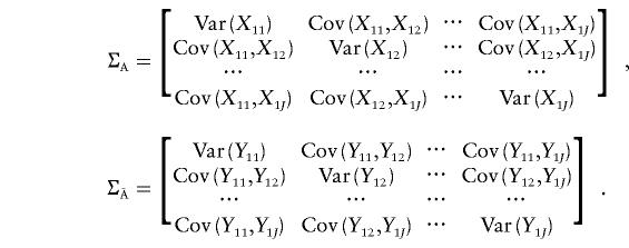It is clear that the covariance matrices Σ_A and depend on the pairwise LD between the marker and trait loci. When , the noncentrality parameter of the T² statistic under the alternative hypothesis is given by

where μ=[μ₁,…,μ_J]^T. Let

G² can be considered to be a genetic-distance measure between two populations that is similar to that proposed by Balakrishnan and Sanghvi (1968). Intuitively, then, the noncentrality parameter λ can be expressed as a function of this genetic distance between the case and control populations;—that is, . In the case in which all pairwise LD is equal to zero, G² is reduced to

and the noncentrality parameter λ is

For a single marker, we have

and

Therefore, the noncentrality parameter and power depend on the sample size and the genetic distance, which, in turn, are a function of allele frequencies and LD between the marker and trait loci.

The classic test statistic for a single-marker case-control study is given by (see Chapman and Wijsman 1998)

where , , , and are the corresponding observed allele frequencies. Its noncentrality parameter, λ_c, is given by

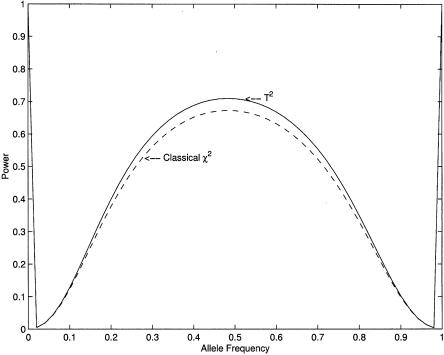
It can be shown (see Appendix B) that λ⩾λ_c. Therefore, for case-control association studies, the proposed T² statistic has higher (or equivalent) power than does the classic T_c statistic. Figure 1 compares the power, for detection of a disease gene, of the T² statistic and the classic χ² statistic. From figure 1, we can see that, in all cases, the power of the T² statistic is higher than that of the classic χ² statistic. However, when the allele frequencies are small, the differences in the power of these two statistics are very small. It can be shown that, even in more complicated situations, such as multiple marker and trait loci, the T² statistic has higher power than does the classic χ² statistic (data not shown).

Figure 1.

Power curves of the T² test and the χ² test, with significance level α=0.0001, as a function of allele frequency, with penetrances assumed to be f₁₁=0.4, f₁₂=0.2, and f₂₂=0.1 and with sample size .

Two-Disease-Loci Model

To further evaluate the power of the T² statistic, we consider two-locus disease models. Assume that there are two disease loci, D and d. Each disease locus has two alleles. The frequencies of the alleles D₁ and D₂ at disease locus D and of the alleles d₁ and d₂ at disease locus d can be denoted by P_D1, P_D2, P_d1, and P_d2, respectively. The frequencies of the genotypes D_uD_v and d_kd_l in the disease and normal populations are denoted by P_DuDv and P_dkdl, respectively. The penetrance of the genotypes D_uD_vd_kd_l will be denoted by f_uvkl. Then, the prevalence of the disease in the population is given by

Denote the indicator variables for the genotypes of the first and second markers for the first individual from the affected population and for the first individual from the unaffected population by X₁₁, X₁₂, Y₁₁, and Y₁₂, respectively. Let

and let

The elements of the vector μ and of the variance-covariance matrices Σ_A and are given in Appendix C. The noncentrality parameter of the T² statistic for the two-locus disease model is then given by

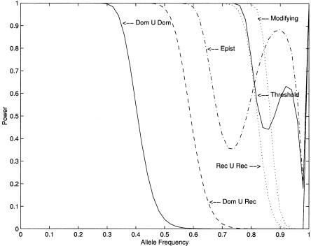
For convenience of presentation, we assume that the two disease loci are unlinked. Table 1 presents six types of two-locus disease models (Neuman and Rice 1992; Schork et al. 1993; Ott 1999). To illustrate the performance of the T² statistic for the detection of disease loci, we plot figure 2, showing the power of the T² statistic as a function of the allele frequency under the six types of two-locus–disease models in table 1.

Table 1.

Penetrance of Given Genotypes for Six Two-Locus Disease Models^[Note]

	Locus d
Model and Locus D	d1d1	d1d2	d2d2
Dom ∪ Dom:
D1D1	f	f	f
D1D2	f	f	f
D2D2	f	f	0
Dom ∪ Rec:
D1D1	f	f	f
D1D2	f	f	f
D2D2	f	0	0
Rec ∪ Rec:
D1D1	f	f	f
D1D2	f	0	0
D2D2	f	0	0
Epistasis or Dom ∩ Dom:
D1D1	f	f	0
D1D2	f	f	0
D2D2	0	0	0
Threshold:
D1D1	f	f	0
D1D2	f	0	0
D2D2	0	0	0
Modifying:
D1D1	f	f	f
D1D2	f	0	0
D2D2	0	0	0

Note.— Adopted from Fan et al. (in press). f is a penetrance.

Figure 2.

Power curves of the T² test, with significance level α=0.0001, as a function of allele frequency, in the case of Dom ∪ Dom, Dom ∪ Rec, Rec ∪ Rec, epistasis, threshold, and modifying models, when , P_D1=P_d1, and f=0.6 are assumed.

The Haplotype T² Statistic

When haplotype information is available, we can define an indicator variable for the alleles of the jth marker on the ith chromosome from the affected population:

Similarly, we define an indicator variable y_Hij for the marker alleles located on the chromosomes from the unaffected population. Following the same development in the genotype T² statistic, we can define the haplotype T² statistic. Let

The covariance matrix is defined as

The haplotype T² statistic is then defined as

To compare the powers of the genotype T² and haplotype T²_H, we can compare their noncentrality parameters, because both T² and T²_H follow a χ²_(J) distribution under the alternative hypothesis. It can be shown that the noncentrality parameter λ of the T² statistic and the noncentrality parameter λ_H of the T²_H statistic are equal (Appendix D).

Therefore, the power of the multilocus T² statistic is the same as that of the haplotype T² statistic. Equivalence of the two statistics is important, because unequivocal haplotypes are usually not available in the majority of case-control studies. Intuitively, this equivalence can be attributed to the fact that the multilocus T² statistic contains the same pairwise LD information in the covariance matrices—that is, Σ_A and —that is contained in the haplotypes.

Search Algorithm

To identify SNP markers (or the combination of SNP markers) that make the greatest contribution to disease risk and drug response, search algorithms are fundamental. In this study, we use a heuristic algorithm that seeks the best combination of SNP markers for risk assessment. The algorithm is based on the sequence-forward floating-selection (SFFS) algorithm of Pudil et al. (1994), which is easy to implement and which requires minimal computation. The SFFS algorithm is based on a sequence-forward–selection algorithm (SFS). The procedures for sequential-forward selection are as follows:

• 1. Compute the desired criterion value for each of the markers, and select the marker with the best value;
• 2. Form all possible two-dimensional vectors that contain the winner from the previous step, and compute the criterion value for each of them and then select the best one;
• 3. Form all three-dimensional vectors expanded from the two-dimensional winners, and select the best one; continue this process until the prespecified dimension of the feature vector—say, l—is reached.

The SFS algorithm requires less computational burden than do other search algorithms, but it suffers from the so-called nesting effect—that is, once a marker is chosen, there is no way for it to be discarded in later steps. To overcome this problem, the SFFS algorithm was proposed. The SFFS algorithm balances the required computational time and overall optimality. (For details, interested readers are referred to Pudil et al. [1994] and Xiong et al. [2001].)

Examples

The proposed T² test was applied to a simulated data set from Genetic Analysis Workshop 12 (GAW12) (Almasy et al. 2001). Simulated data were provided for an isolated population founded ∼20 generations ago by 100 individuals from the general population. Unrelated cases and control subjects () were obtained by selection of founders and their spouses from 23 extended pedigrees. Sequence data are available for a major gene, MG6 on chromosome 6, that directly influences affection status of the individuals. MG6 is known to account for 25.3% of disease liability, and, in the GAW12 data, the sequence data are labeled “GENE 1.” Site 557 was identified as the SNP closely related to disease liability. The P values of the T² statistic and of the classic χ² statistic, for testing the association between SNP markers and affection status that are included within GENE 1 are summarized in table 2. We can see from table 2 that both the T² test and the χ² test identified a common set of SNP markers showing significant association with affection status but that, in all cases, the T² test had smaller P values than did the χ² test. The T² test identified site 557 as having the smallest P value. Since strong LD exists between many SNP markers within GENE 1 (Czika et al. 2000; Huang et al. 2001), both the T² test and the χ² test identified a number of SNP markers that had small P values.

Table 2.

Results of the T² Test and the Classic χ² Test, When Applied to Simulated Data within Gene 1 from GAW12^[Note]

	P, by Type of Test
Position	T2	χ2	r2
557	6.6 × 10 −14	3.04 × 10−11
1553	6.6 × 10−14	3.04 × 10−11	.97
2619	6.6 × 10−14	3.04 × 10−11	.97
3456	6.6 × 10−14	3.04 × 10−11	.97
3573	6.6 × 10−14	3.04 × 10−11	.97
3742	6.6 × 10−14	3.04 × 10−11	.97
3835	6.6 × 10−14	3.04 × 10−11	.97
3853	6.6 × 10−14	3.04 × 10−11	.97
76	2.66 × 10−13	9.67 × 10−11	.99
11180	2.86 × 10−13	3.04 × 10−11
2923	6.41 × 10−13	2.44 × 10−11	.86
5757	8.019 × 10−13	2.12 × 10−11	.93
7281	8.019 × 10−13	2.12 × 10−11	.93
1478	1.199 × 10−12	4.59 × 10−11	.85
4471	1.2832 × 10−11	1.43 × 10−10	.86
4752	1.2832 × 10−11	1.43 × 10−10	.86
2942	1.5017 × 10−11	3.93 × 10−10	.91
3534	1.16706 × 10−8	5.41 × 10−8	.73
3653	1.16706 × 10−8	5.41 × 10−8	.73
5094	1.16706 × 10−8	5.41 × 10−8	.73
5244	1.16706 × 10−8	5.41 × 10−8	.73
2732	1.42422 × 10−8	3.02 × 10−8	.66
2853	1.42422 × 10−8	3.02 × 10−8	.66
596	2.28199 × 10−8	5.41 × 10−8	.73
5542	4.81874 × 10−8	1.36 × 10−7	.71
189	6.05394 × 10−8	1.40 × 10−7	.72
12185	8.64 × 10−8	3.54 × 10−7
13074	8.64 × 10−8	4.54 × 10−7
5688	8.73906 × 10−8	1.36 × 10−7	.71
4602	9.36796 × 10−8	2.12 × 10−7	.66
4688	9.36796 × 10−8	2.12 × 10−7	.66

Note.— Data are from Almasy et al. (2001).

Table 3 shows (1) the results of the T² test for 17 two-SNP combinations that have P values <10⁻¹⁴ and (2), of all possible three-SNP combinations, the top 15 that have the smallest P value. Two features are evident from table 3: first, the P values of the optimal combination of two or three SNPs are smaller than that of each single SNP in the combination; second, an individual SNP may have a large P value, but its combinations with other SNPs may have a very small P value.

Table 3.

Results of the T² Test Applied to Simulated Data within GENE 1 from GAW12, When Two or Three SNPs Are Used^[Note]

1st SNP		2d SNP		3d SNP
Position	P	Position	P	Position	P	P for 1st and 2d SNPs or for 1st, 2d, and 3d SNPs
557	6.60 × 10−14	9150	3.55 × 10−7			5.55 × 10−16
76	2.66 × 10−13	9150	3.55 × 10−7			2.00 × 10−15
1553	6.60 × 10−14	9150	3.55 × 10−7			5.55 × 10−15
2619	6.60 × 10−14	9150	3.55 × 10−7			5.55 × 10−15
3456	6.60 × 10−14	9150	3.55 × 10−7			5.55 × 10−15
3573	6.60 × 10−14	9150	3.55 × 10−7			5.55 × 10−15
3742	6.60 × 10−14	9150	3.55 × 10−7			5.55 × 10−15
3835	6.60 × 10−14	9150	3.55 × 10−7			5.55 × 10−15
3853	6.60 × 10−14	9150	3.55 × 10−7			5.55 × 10−15
557	6.60 × 10−14	4315	1.83 × 10−6			6.99 × 10−15
1553	6.60 × 10−14	4315	1.83 × 10−6			6.99 × 10−15
2619	6.60 × 10−14	4315	1.83 × 10−6			6.99 × 10−15
3456	6.60 × 10−14	4315	1.83 × 10−6			6.99 × 10−15
3573	6.60 × 10−14	4315	1.83 × 10−6			6.99 × 10−15
3742	6.60 × 10−14	4315	1.83 × 10−6			6.99 × 10−15
3835	6.60 × 10−14	4315	1.83 × 10−6			6.99 × 10−15
3853	6.60 × 10−14	4315	1.83 × 10−6			6.99 × 10−15
76	2.66 × 10−13	4315	1.83 × 10−6	9150	1.40 × 10−5	1.11 × 10−16
557	6.60 × 10−14	5654	1.24 × 10−7	9150	1.40 × 10−5	1.11 × 10−16
557	6.60 × 10−14	5688	8.74 × 10−8	9150	1.40 × 10−5	1.11 × 10−16
557	6.60 × 10−14	5721	1.24 × 10−7	9150	1.40 × 10−5	1.11 × 10−16
557	6.60 × 10−14	5922	1.24 × 10−7	9150	1.40 × 10−5	1.11 × 10−16
557	6.60 × 10−14	6912	1.24 × 10−7	9150	1.40 × 10−5	1.11 × 10−16
557	6.60 × 10−14	7577	1.24 × 10−7	9150	1.40 × 10−5	1.11 × 10−16
557	6.60 × 10−14	7654	3.76 × 10−2	9150	1.40 × 10−5	1.11 × 10−16
557	6.60 × 10−14	7890	1.24 × 10−7	9150	1.40 × 10−5	1.11 × 10−16
557	6.60 × 10−14	9341	1.24 × 10−7	9150	1.40 × 10−5	1.11 × 10−16
1553	6.60 × 10−14	5757	8.02 × 10−12	7890	3.76 × 10−2	1.11 × 10−16
1553	6.60 × 10−14	7281	8.02 × 10−12	7890	3.76 × 10−2	1.11 × 10−16
557	6.60 × 10−14	1407	5.94 × 10−1	9150	1.40 × 10−5	2.22 × 10−16

Note.— Data are from Almasy et al. (2001).

The proposed T² test was also applied to a real data set of cases of scleroderma, or systemic sclerosis (SSC) (X. Zhou, F. K. Tan, J. D. Reveille, C. Ahn, A. Wang, and F. C. Arnett, personal communication). SSC is a multisystem disease of unknown etiology and is characterized by cutaneous and visceral fibrosis, small-blood-vessel damage, and autoimmune features (Medsger 1997; X. Zhou, F. K. Tan, J. D. Reveille, C. Ahn, A. Wang, and F. C. Arnett, personal communication). Three SNP markers—SPARC 998, SPARC 1551, and SPARC 1992—were genotyped in 20 unrelated patients with SSC and in 75 normal control subjects from the Oklahoma Choctaw population. It has been reported that, in this population, (a) the clinical disease pattern is relatively homogeneous and (b) the prevalence of SSC in this population is high (X. Zhou, F. K. Tan, J. D. Reveille, C. Ahn, A. Wang, and F. C. Arnett, personal communication). To further evaluate the performance of the T² test, both the T² test and the χ² test were applied to the samples from the Oklahoma Choctaw, to examine association between the SPARC gene and SSC. Table 4 presents the results. It is evident from table 4 that marker SPARC 998 has a T²-associated P value that is much smaller than that associated with the classic χ² test. It has been reported that expression of the SPARC gene is ∼2.5-fold and ∼5-fold increased, respectively, when cDNA microarrays and western-blot analysis are used, in case-control comparisons for SSC (X. Zhou, F. K. Tan, J. D. Reveille, C. Ahn, A. Wang, and F. C. Arnett, personal communication). The SPARC gene is being increasingly recognized as playing a variety of roles in tissue development, remodeling, and fibrosis (Motamed 1999).

Table 4.

Test for Association between SPARC SNP Markers and SSC in Oklahoma Choctaw, by the T² Test and the χ² Test^[Note]

	P, by Type of Test
Marker	T2	χ2
SPARC 998	.003886	.01108
SPARC 1551	.04859	.1198
SPARC 1922	.1889	.1915

Note.— Data are from X. Zhou, F. K. Tan, J. D. Reveille, C. Ahn, A. Wang, and F. C. Arnett (personal communication).

Discussion

In this study, we have proposed a generalized T² statistic to relate DNA sequence variations to the occurrence of disease. We show that the noncentrality parameter of the T² statistic is larger than that of the well-known χ² statistic, indicating that the T² statistic has greater power than does the χ² statistic. In addition, simulation studies and examples with real data demonstrate that, for case-control studies, the P value of the T² test is smaller than that of the χ² test.

The proposed generalized T² statistic has utility in three areas of contemporary human genomic analysis. First, there is general interest in using a dense set of SNPs spanning each of the chromosomes, to localize genes via genomewide association analyses. For such association studies to be effective, it is not necessary that the SNPs be the disease-susceptibility loci; rather, the SNPs may aid in identification of the location of a disease-susceptibility locus, on the basis of LD between the SNP marker loci and nearby disease-susceptibility loci. The magnitude of LD among SNPs (including disease-susceptibility loci) is largely determined by the recombination rates among loci and by stochastic sampling variation, including genetic drift, migration, and sampling. Therefore, association between an SNP (or SNPs) and a trait of interest is generally attributable to LD between the SNP (or SNPs) and a disease-susceptibility locus. Such association may indicate proximity of the inferred disease-susceptibility locus to the SNP marker locus.

The second area in which the proposed statistic has utility is in analysis of the spectrum of variation within a gene, to identify sites or combinations of sites influencing the trait of interest. Variations at these sites are candidates for further experimental and functional studies. An association-mapping perspective is of little utility in this situation, because the recombination rate among sites is practically zero. In this case, one should first identify the complete menu of variable sites within the gene and then consider the ability of these sites to predict levels or prevalence rates of the phenotype of interest. Recent studies (e.g., see Horikawa et al. 2000) have indicated that there are not sufficient data to predict a priori which sites (e.g., cSNPs) are likely to predict and which are likely not to predict.

The third application of the T² analysis is to the development of a more comprehensive vision of the genetic architecture (see Boerwinkle et al. 1986) of a trait. It is widely accepted that risk to a common disease is influenced by multiple genes and that these genes are interacting both among themselves and with environmental factors. One of the goals of studying the genetics of common diseases is to identify the contributing genes and mutations and to characterize their interaction as they combine with other agents to influence disease risk. To achieve this goal, it is necessary to have methods that evaluate multiple loci—and their interactions—simultaneously. The proposed T² statistic, by virtue of the fact that it simultaneously considers the effects of multiple loci and does not assume additivity among those effects, is an important step in this direction. Future developments will include (1) extension of the T² method to quantitative traits and (2) stepwise site-selection procedures. One aspect of considerable interest in the area of genome association studies is the use of haplotype information. Recently, some have argued that haplotypes may be the relevant functional unit in the consideration of genotype-phenotype relationships (Drysdale et al. 2000). In addition, haplotype information can facilitate a cladistic approach to genotype-phenotype relationships (Templeton et al. 1987). In the case of the T² test, haplotype information has here been shown not to lend additional information about genotype-phenotype relationships, relative to multilocus genotype information. Initially, this result was surprising. However, on further investigation it was realized that the sample variance-covariance matrix, S, contains the pairwise relationships among loci. Therefore, the T² statistic captures the pairwise-association information found in haplotypes. Higher-order associations, however, may not be included in the regular T² statistic, indicating that the T²_H statistic may have advantages in those situations.

LD analyses and association mapping are powerful tools for contemporary human genetics. Efforts to build a collection of SNP markers in all genes of the human genome (e.g., see The International SNP Map Working Group 2001 ) and advances in genotyping technologies bode well for large-scale applications in the near future. Such undertakings are not without complications, however. The cost-per-locus test for SNPs remains high. The pattern of LD may vary considerably between populations. And there is a further need to develop, evaluate, and apply novel methods for relating the considerable genomic information to risk of disease—methods such as the T² test proposed here.

Appendix A :

Assuming Hardy-Weinberg equilibrium, we can calculate and as follows:

Therefore, we have

Next, we calculate the variance-covariances, Var(X_j) and Cov(X_j,X_j^′). Note that

where δ_jj^′(A)=P_BjBj^′(A)-P_Bj(A)P_Bj^′(A).

Combining the above equations yields Cov(X_ij,X_ij^′)=E[X_ijX_ij^′]-E[X_ij]E[X_ij^′]=2δ_jj^′(A). It is not difficult to see that Var(X_ij)=E[X²_ij]-(E[X_ij])²=P²_Bj(A)+P²_bj(A)-[P_Bj(A)-P_bj(A)]²=2P_Bj(A)P_bj(A). Similarly, we have .

Appendix B :

Note that P_b(A)=1-P_B(A) and . Thus,

However, , which implies that

Therefore, we have

It follows that

But, when , λ is reduced to

Appendix C:

To calculate the noncentrality parameter, λ₂, we begin with the calculation of the frequencies of the genotypes at the two disease loci, in the affected population and in the control populations. It follows from the definition of the genotype frequencies in the disease population that

Similarly, we have

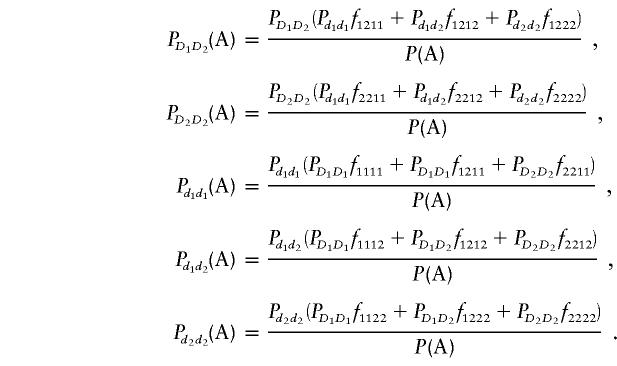Let be the probability that an individual with genotypes D_iD_j and d_kd_l is unaffected. By an argument similar to that used above, we obtain

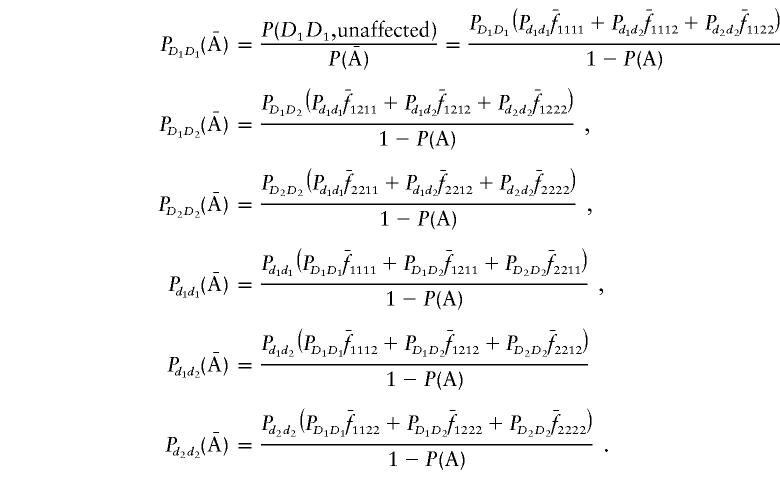Now we calculate the expectation of the indicator variables X₁₁ and Y₁₁. Using the definition of the indicator variable, we have

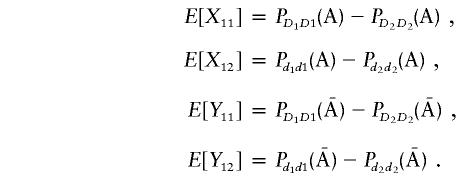Thus, the vector μ can be calculated by μ=(E[X₁₁]-E[Y₁₁],E[X₁₂]-E[Y₁₂])^T. Next we calculate the variance-covariance matrix Σ_A. It is easy to see that

Therefore, we obtain

and

Appendix D :

If we assume Hardy-Weinberg equilibrium, we find that it is not difficult to show that

Thus, μ_H=(μ_H1,…,μ_HK)^T; Σ_HA=(1/2)Σ_A and . The noncentrality parameter λ_H is then given by

References

- Almasy L, Terwilliger JD, Nielsen D, Dyer TD, Zaykin D, Blangero J (2001) GAW12: simulated genome scan, sequence, and family data for a common disease. Genet Epidemiol 21:S332–S338 [DOI] [PubMed] [Google Scholar]
- Balakrishnan V, Sanghvi LD (1968) Distance between populations on the basis of attribute data. Biometrics 24:859–865 [Google Scholar]
- Bhat A, Lucek PR, Ott J (1999) Analysis of complex traits using neural networks. Genet Epidemiol 17 Suppl 1:S503–507 [DOI] [PubMed] [Google Scholar]
- Boerwinkle E, Chakraborty R, Sing CF (1986) The use of measured genotype information in the analysis of quantitative phenotypes in man. I. Models and analytical methods. Ann Hum Genet 50:181–194 [DOI] [PubMed] [Google Scholar]
- Chapman NH, Wijsman EM (1998) Genome screens using linkage disequilibrium tests: optimal marker characteristics and feasibility. Am J Hum Genet 63:1872–1885 [DOI] [PMC free article] [PubMed] [Google Scholar]
- Czika WA, Weir BS, Edwards SR, Thompson RW, Nielsen DM, Brocklebank JC, Zinkus C, Martin ER, Hobler KE (2001) Applying data mining techniques to the mapping of complex disease genes. Genet Epidemiol 21 Suppl 1:S435–S440 [DOI] [PubMed] [Google Scholar]
- Drysdale CM, McGraw DW. Stack CB, Stephens JC, Judson RS, Nandabalan K, Arnold K, Ruano G, Liggett SB (2000) Complex promoter and coding region β2-adrenergic receptor haplotypes alter receptor expression and predict in vivo responsiveness. Proc Natl Acad Sci USA 97:10483–10488 [DOI] [PMC free article] [PubMed] [Google Scholar]
- Fan R, Floros J, Xiong MM. Transmission disequilibrium test of two unlinked disease loci: application to respiratory distress syndrome. Adv Appl Stat (in press) [Google Scholar]
- Gray IC, Campbell DA, Spurr NK (2000) Single nucleotide polymorphisms as tools in human genetics. Hum Mol Genet 9:2403–2408 [DOI] [PubMed] [Google Scholar]
- Hotelling H (1931) The generalization of student’s ratio. Ann Math Stat 2:360–378 [Google Scholar]
- Horikawa Y, Oda N, Cox NJ, Li X, Orho-Melander M, Hara M, Hinokio Y, Lindner TH, Mashima H, Schwarz PEH, et al (2000) Genetic variation in the gene encoding calpain-10 is associated with type 2 diabetes mellitus. Nat Genet 26:163–175 [DOI] [PubMed] [Google Scholar]
- Huang QQ, Marrison AC, Boerwinkle E (2001) Linkage disequilibrium structure and its impact on the localization of a candidate functional mutation. Genet Epidemiol 21: S620–S625 [DOI] [PubMed] [Google Scholar]
- International SNP Map Working Group, The (2001) A map of human genome sequence variation containing 1.42 million single nucleotide polymorphisms. Nature 409:928–933 [DOI] [PubMed] [Google Scholar]
- Li X, Rao S, Elston RC, Olson JM, Moser KL, Zhang T, Guo Z (2001) Locating the genes underlying a simulated complex disease by discriminant analysis. Genet Epidemiol 21 Suppl 1:S516–521 [DOI] [PubMed] [Google Scholar]
- Longmate JA (2001) Complexity and power in case-control association studies. Am J Hum Genet 68:1229–1237 [DOI] [PMC free article] [PubMed] [Google Scholar]
- Medsger TA Jr (1997) Systemic sclerosis (scleroderma): clinical aspects. In: Koopman WJ (ed) Arthritis and allied conditions: a textbook of rheumatology. Williams & Wilkins, Baltimore 1433-1464 [Google Scholar]
- Motamed K (1999) SPARC (osteonectin/BM-40). Int J Biochem Cell Biol 31:1363–1366 [DOI] [PubMed] [Google Scholar]
- Neuman RJ, Rice JP (1992) Two-locus models of diseases. Genet Epidemiol 9:347–365 [DOI] [PubMed] [Google Scholar]
- Ott J (1999) Analysis of human genetic linkage, 3d ed. Johns Hopkins University Press, Baltimore [Google Scholar]
- Pudil P, Novovicova J, Kittler J (1994) Floating search methods in feature selection. Pattern Recognition Lett 15:1119–1125 [Google Scholar]
- Risch N, Merikangas K (1996) The future of genetic studies of complex human diseases. Science 273:1516–1517 [DOI] [PubMed] [Google Scholar]
- Schork NJ, Boehnke M, Terwilliger JD, Ott J (1993) Two-trait-locus linkage analysis: a powerful strategy for mapping complex genetic traits. Am J Hum Genet 53:1127–1136 [PMC free article] [PubMed] [Google Scholar]
- Sherriff A, Ott J (2001) Applications of neural networks for gene finding. Adv Genet 42:287–297 [DOI] [PubMed] [Google Scholar]
- Templeton AR, Boerwinkle E, Sing C (1987) A Cladistic analysis of phenotypic associations with haplotypes inferred from restriction endonuclease mapping. I. Basic theory and an analysis of alcohol dehydrogenase activity in drosophila. Genetics 117:343–351 [DOI] [PMC free article] [PubMed] [Google Scholar]
- Xiong MM, Fang XZ, Zhao JY (2001) Biomarker identification by feature wrappers. Genome Res 11:1878–1887 [DOI] [PMC free article] [PubMed] [Google Scholar]
- Zhang HP, Bonney G (2000) Use of classification trees for association studies. Genet Epidemiol 19:323–332 [DOI] [PubMed] [Google Scholar]