Convergent Random Forest Predictor: Methodology for predicting drug response from genome-scale data applied to anti-TNF response

Abstract

Biomarker development for prediction of patient response to therapy is one of the goals of molecular profiling of human tissues. Due to the large number of transcripts, relatively limited number of samples, and high variability of data, identification of predictive biomarkers is a challenge for data analysis. Furthermore, many genes may be responsible for drug response differences, but often only a few are sufficient for accurate prediction. Here we present an analysis approach, the Convergent Random Forest (CRF) method, for the identification of highly predictive biomarkers. The aim is to select from genome-wide expression data a small number of non-redundant biomarkers that could be developed into a simple and robust diagnostic tool. Our method combines the Random Forest classifier and gene expression clustering to rank and select a small number of predictive genes. We evaluated the CRF approach by analyzing four different data sets. The first set contains transcript profiles of whole blood from rheumatoid arthritis patients, collected before anti-TNF treatment, and their subsequent response to the therapy. In this set, CRF identified 8 transcripts predicting response to therapy with 89% accuracy. We also applied the CRF to the analysis of three previously published expression data sets. For all sets, we have compared the CRF and recursive support vector machines (RSVM) approaches to feature selection and classification. In all cases the CRF selects much smaller number of features, five to eight genes, while achieving similar or better performance on both: training and independent testing sets of data. For both methods performance estimates using cross-validation is similar to performance on independent samples. The method has been implemented in R and is available from the authors upon request: Jadwiga.Bienkowska@biogenidec.com.

Introduction

Advances in high-throughput, genome-wide transcript profiling technologies make it possible to investigate how molecular features of patients correlate with clinical disease subtypes and response to treatment. Computational and statistical analysis of transcript profiling (or proteomic) data from large patient populations can be used to find classifiers that differentiate among patient groups of clinical interest. One goal of this type of research is the development of molecular diagnostics that predict which drugs will be most beneficial to specific patients. Recently, several statistical methods [1; 2; 3] have been introduced to address the problems of classification and feature selection using gene expression data. The classification of a clinical parameter, such as disease subtype or responder vs non-responder, is accomplished using several molecular features, i.e. gene expression. One of the challenges is to design a robust classification algorithm that will perform well on unseen data. Another challenge is to select features (genes) that are unique, consistent, and non-redundant with a high aggregate predictive accuracy. Identifying a small set of genes is especially useful for the development of a clinical diagnostic where simple and robust technologies are needed.

In this paper, we introduce a new methodology to construct a robust classifier as well as to select the minimum number of genes with maximum prediction performance. For classification we used the random forest (RF) algorithm, a machine learning technique introduced by Breiman [4], shown to outperform most of the other classification techniques in different tasks [2; 5; 6; 7; 8; 9]. The RF approach builds a number of decision trees ntree from randomly selected sets of genes-mtry and about 2/3 of the samples. The rest of the samples are called out-of-bag samples and the error rate calculated from the prediction of these samples is called the out-of-bag error (OOB error). OOB estimate of error rate was reported to be quite accurate and unbiased [10] since the information provided by out-of-bag samples is not used to build the trees. The RF approach also calculates the influence of each variable (e.g. gene expression) to the predictions, called variable importance [11].

Although the RF is a very powerful statistical method, the challenges presented by gene expression data sets are not easily overcome by a standard application of the algorithm. The main challenge is the curse of dimensionality presented by gene expression data with relatively few samples (∼100 patients) to be classified by a much larger set of features (30,000 gene expression values). Thus, simultaneous reduction of the dimensionality of the data and retention of the differentiating features is one of the objectives of our approach. We address these challenges by first identifying the optimal algorithm parameters for a data set and then by introducing a new method for selection of the most predictive features. We identify the best features by applying a converging RF algorithm and select the most predictive genes with cluster cutting, where gene expression correlations are taken into account. The RF algorithm was reported to perform well with its default parameter mtry (number of random variables) [10], however there is no study comprehensively evaluating the dependence of its performance on the parameters. Here, we present a general methodology to select the best parameters to construct a stable RF classifier.

Another challenge in designing the best predictor is feature (gene transcript) selection. Feature selection algorithms typically use one of two approaches: (1) recursive gene filtering/shaving and (2) frequency-based gene ranking. Recursive gene filtering has been applied by van't Veer [12], in a variant of support vector machines (SVM) known as SVM recursive feature elimination (SVM-RFE) [1], and also in the context of Random Forest [13; 14]. Zhang et al. [15] developed a recursive support vector machine (R-SVM) algorithm that is similar to SVM-RFE but selects important features based on frequency. They showed that R-SVM outperforms SVM-RFE in the robustness to noise as well as in recovery of informative features, and has better accuracy on independent test data. Here, we define a frequency-based Gene Predictive Index that is used for gene selection.

In this paper, we introduce an algorithm that first constructs a robust random forest classifier with optimal parameters and then selects the minimum number of genes with maximum accuracy in predicting response. To construct a stable classifier we evaluate the effects of different parameters on the random forest error rate, and introduce a methodology to select the best parameters. With the optimal parameters we find a set of predictive genes. To select the minimum number of genes from this set, we introduce a novel clustering-based gene selection method that uses frequency to rank genes. The frequency ranking ensures that selected genes are consistently important in prediction, while the clustering approach selects an uncorrelated and non-redundant small set of genes with high prediction capability. The variability of the lists of the most predictive genes has been noted previously [16] and was shown to depend on the training set. It has been also shown that, despite this variability, different best gene sets perform well on independent samples sets [17]. Here, we use the random sampling of the RF to capture this variability and identify all of the best predictive genes.

We applied our algorithm to a data set of whole blood gene expression profiles for 46 Rheumatoid Arthritis patients. The blood was collected from the patients before the start of anti-TNF therapy with one of the three approved drugs: etaneracept, inflixmab, or adalimumab. Patients' response to therapy was assessed after a 3 months treatment. The CRF approach identified a pre-treatment eight-gene signature that predicts response to therapy with 89% accuracy and has been replicated with a small independent set of samples. This finding demonstrates the feasibility of development of a molecular diagnostic for use in the medical care of RA patients with anti-TNF therapies.

To show the general utility of our approach we have also applied the CRF to three previously published expression data sets and have compared with the recursive SVM (RSVM) method for feature selection and classification [15]. We have evaluated the performance of both methods using independent testing sets of samples that were not used in any step in the training process or feature selection. In all cases, the CRF selects a much smaller number of features (5-8 genes) as compared to RSVM (60-80 genes) and in most cases has better performance as measured by the area under the receiver operating characteristic (ROC) curve (AUC).

Results

Overview of the method

We consider as an input data a set of gene expression profiles representing N_s samples classified into response or disease categories R_s. N_g is the number of transcripts relevant to the tissue type and disease that are to be considered as predictive features. Design of the Convergent Random Forest Predictor follows in three main steps. (1) Selection of the Random Forest parameters optimal for the dataset. (2) Identification of subset NP_g < N_g genes consistently predictive of the response categories. (3) Ranking and selection of most predictive genes MP_g ≪ NP_g and selecting the final classifier. Here, NP_g is the number of predictive genes and MP_g is the number of most predictive genes from which the predictors are built.

Step 1: Finding optimal parameters for random forest

Two parameters are important in the random forest algorithm: the number of trees used in the forest (ntree) and the number of random variables used in each tree (mtry). Initial investigation of the OOB errors determined that performance of the classifier is much more sensitive to the number of trees than the mtry values. Thus we first set the mtry to the default value ${\mathit{\text{mtry}}}_d=\sqrt{{\mathrm{N}}_{\mathrm{g}}}$ and search for the optimal ntree value. To find the number of trees that correspond to a stable classifier, we build RF with different ntree values i.e. ntree_i= {1, 500, 1000…., 120,000}. We build 10 RF classifiers for each ntree value, record the OOB error rate and calculate the median and standard deviation of the error rate, m.OOB[ntree_i] and sdv.OOB[ntree_i]. First we identify the minimal value of ntree where m.OOB[ntree_i] and sdv.OOB[ntree_i] stabilize:

$${\mathit{\text{ntree}}}_O=\underset{{\mathit{\text{ntree}}}_i}{argmax}\left(\begin{array}{c}{argmin}_{{\mathit{\text{ntree}}}_i}(m.\mathit{\text{OOB}}[{\mathit{\text{ntree}}}_i]\le {min}_{{\mathit{\text{ntree}}}_j>{\mathit{\text{ntree}}}_i}(m.\mathit{\text{OOB}}[{\mathit{\text{ntree}}}_j]))\\ {argmin}_{{\mathit{\text{ntree}}}_i}(\mathit{\text{sdv}}.\mathit{\text{OOB}}[{\mathit{\text{ntree}}}_i]\le {min}_{{\mathit{\text{ntree}}}_j>{\mathit{\text{ntree}}}_i}(\mathit{\text{sdev}}.\mathit{\text{OOB}}[{\mathit{\text{ntree}}}_j]))\end{array}\right)$$ (1)

We set the ntree value to the optimal as described above and proceed to the search for optimal mtry.

To find the optimum mtry, we apply a similar procedure such that RF is run 10 times for a range of mtry values which consist of multiples of the default ${\mathit{\text{mtry}}}_d=\sqrt{{\mathrm{N}}_{\mathrm{g}}}$ starting from 0.05×mtry_d up to mtry = N_s with increments of 0.05. At each run the OOB error rate is recorded. The optimum mtry value(s) is selected for which the error rate has stabilized and reached minimum. The following formula defines the mtry values that correspond to the minimums:

$${\mathit{\text{mtry}}}_O=\underset{{\mathit{\text{mtry}}}_k\in \{{\mathit{\text{mtry}}}_m\}}{argmin}(\{{\mathit{\text{mtry}}}_m\})=\underset{{\mathit{\text{mtry}}}_i(i=2\dots N_s)}{argmin}(m.\mathit{\text{OOB}}[{\mathit{\text{mtry}}}_i]),\underset{{\mathit{\text{mtry}}}_k\in \{{\mathit{\text{mtry}}}_m\}}{argmin}(|m.\mathit{\text{OOB}}[{\mathit{\text{mtry}}}_k]-m.\mathit{\text{OOB}}[{\mathit{\text{mtry}}}_{k-1}]|+|m.\mathit{\text{OOB}}[{\mathit{\text{mtry}}}_i]-m.\mathit{\text{OOB}}[{\mathit{\text{mtry}}}_{k+1}]|+\mathit{\text{sdv}}.\mathit{\text{OOB}}[{\mathit{\text{mtry}}}_k])$$ (2)

where m.OOB[mtry_i] is the median OOB error rate and sdv.OOB[mtry_i] is the standard deviation. Equation 2 selects mtry_O values that satisfy both the lowest error rate and the highest stability. In practice this equation may identify more than one optimal mtry_O value. For the optimal values that differ by one we select the smaller mtry_O.

Step 2: Selecting genes consistently important in prediction

With the optimal values of ntree_O and mtry_O as parameters, we apply the Convergent Random Forest algorithm to select predictive genes. The RF is run 10 times with each variable (gene) assessed by its importance. From each run we record genes with positive importance, those that improve the prediction accuracy. Next, we select genes common for all 10 runs. We iterate over the batches of 10 RFs each time recording the predictive gene list Pⁱ_g from the batch i as only those that are in common with the previous batch i-1, P_gⁱ ⊆ P_g^i-1 . We stop the iteration at i=imax, when the list from subsequent batches are identical P_g^imax =P_g^imax-1. The P^imax_g is the list of consistently predictive genes. This procedure is repeated for all mtry_O and the set of predictive genes NP_g is the set common to all values.

Step 3: Selecting minimum number of genes with maximum prediction accuracy

The last step of the algorithm identifies among NP_g genes selected in step 2 those that predict the responses with maximum accuracy. The gene selection/filtering algorithm derives from the observation that predictive genes correlate with each other and thus the complete list of predictive genes includes redundancies. Moreover, the response signal encoded in each expression value is confounded by noise and combining many genes in the predictor accumulates the noise. For selecting the best predictive transcripts (genes) we apply two approaches. Both approaches use the importance of the gene as calculated by the RF. The first approach, selection by importance, starts with the most important gene, adds one gene at a time and calculates the OOB-error. The second, selection with clustering approach starts with genes clustered according to their expression correlation across the samples, then we recursively cut the cluster into k sub-clusters and select from each sub-cluster the gene with the highest rank by importance. For each k we build a predictor from the selected genes and calculate the OOB error. This procedure is repeated several times and each time the set of predictor genes with smallest OOB-error is recorded. In this step we use the default mtry value that is equal to $\sqrt{{\mathit{\text{NP}}}_g}$.

Below is the pseudo-code for the two selection procedures. First we rank the genes g₁, g₂,‥, g_n, according to variable importance in decreasing order with r_i denoting the rank of the gene g_i.

Selection of best predictor genes based on importance ranking

1. Set x = 1.

2. Select x top genes $G^x=\underset{i}{\cup }\{g_i;r_i\le x\}$ and calculated OOB[x] error for gene set G^x

3. Set x = x + 1. Repeat from Step 3 until x = n.

4. $x_{min}=\underset{x}{argmin}(\mathit{\text{OOB}}[x])$. There can be several values of x with the lowest error.

Selection based on clustering

1. Cluster the genes using the correlation of the gene expression values as the distance matrix. Set the number of clusters to k = 2.

2. Cut the dendrogram into k clusters, and select the highest ranking gene from each cluster. Those genes make the k-clusters gene set $G^k=\underset{j=1}{\overset{k}{\cup }}arg\underset{g_i\in C^j}{max}(r_i)$, where C^j denotes the j-th cluster (see supplementary figure 4). Next, calculate OOB[k] error for gene set G^k.

3. Set k = k+1. Repeat from Step 2 until k = min(x_min) (see Selection based on importance ranking)

4. $k_{min}=\underset{k}{argmin}(\mathit{\text{OOB}}[k])$. Select k-genes that have minimum OOB error rate.

Ranking the most predictive genes with gene predictive index (GPI)

For ranking the most predictive genes we iterate over the following procedure and record results from each iterationi.

• Select genes based on importance ranking and minimal error rate. Let $G_i^{x_{min}}$ denote the set of selected genes with minimal error rate OOB[x_min] and $|G_i^{x_{min}}|$ the cardinality of this set.

• Select genes based on clustering and minimal error rate. Let $G_i^{k_{min}}$ denote the set of selected genes with minimal error rate OOB[k_min] and $|G_i^{k_{min}}|$ the cardinality of this set.

The final set of most predictive genes MP_g is the union of all best gene subsets identified in the iterations:

$${\mathit{\text{MP}}}_g=\underset{i}{\cup }{G}_i^{x_{min}}\cup G_i^{k_{min}}$$ (3)

The Gene Predictive Index (GPI) for each gene g from the MP_g set is given by the following formula:

$$\mathit{\text{GPI}}(g)=(\sum _i\frac{1-\mathit{\text{OOB}}\left[x_{min}\right]}{|G_i^{x_{min}}|}+\sum _i\frac{1-\mathit{\text{OOB}}[k_{min}]}{|G_i^{k_{min}}|})/max(i)$$ (4)

Thus if the number of most predictive genes including gene g identified in an iteration is small, that gene is given a higher index. Moreover, as the frequency of appearance of the gene in the runs increases, GPI of the gene also increases (through summation). Genes are ranked according to GPI in decreasing order. The maximum value of the GPI is 2 in a hypothetical best case when a perfect prediction (zero error) is obtained with a single gene transcript. As the final step in constructing the predictor we rank genes by the GPI and adding one at the time we calculate the OOB error for the first k-best genes. The final predictor is the one with the smallest error and number of genes. In practice this number is a fraction of the total number of all the best genes ranked by the GPI.

Example I: Prediction of response to TNF-blockade in Rheumatoid Arthritis

We applied the method of designing a Convergent Random Forest Predictor to gene expression profiles of whole blood samples from rheumatoid arthritis patients provided by the Autoimmune Biomarkers Collaborative Network (ABCoN). The blood was collected before patients began TNF-blockade treatment with adalimumab, etanercept, or infliximab. Patients' response, or the change in disease activity, was measured after 14 weeks according to standards of clinical practice. The details about the sample collection, processing, and definition of responsive and non-responsive patients are in Supplementary Material. Our initial gene selection procedure is very stringent and in this case has the false discovery rate of 10^-10. Initial data processing and gene filtering resulted in 166 gene transcripts that are significantly correlated with anti-TNF response, as described in Supplementary Materials and Methods. Starting from 166 transcripts, our primary goal was to find a stable predictor with a minimum number of genes and maximum performance. The accuracy of the RF predictor constructed with 166 transcripts is 68%. Similar accuracy (76%) is achieved with 36 genes that are significantly differentially expressed between responders and non-responders at pre-treatment visit. This level of accuracy is insufficient to pursue the development of clinical diagnostic tools that would clearly benefit patients. To support a recommendation to change treatment to a different drug, a predictive accuracy of more than 80% is desirable. To improve the prediction accuracy to >80%, we applied the Convergent Random Forest Predictor design method to this data set.

Selecting optimal parameters

We searched for the optimum number of trees with a stable classifier i.e. the performance does not change as more trees are added to the forest. For this we ran RF 10 times for different ntree values and default mtry =13, each time recording the OOB error rate. The median and the standard deviation (std) across these 10 runs and different ntree values are shown in supplementary Figure S1a and S1b, respectively. In this data set the median error rate stabilized quickly while the standard deviation continued to decline as more trees were added to the forest. Therefore, the application of equation (1) selected the optimal ntree after which the standard deviation stabilized (Fig S1.b) ntree_O = 15400. Since small differences in the number of trees have no effect on error rates, for simplicity we choose ntree_O=16,000 for the next step. The question arises whether we could be over-fitting with this number of trees. Two things guard us against over-fitting; first each step of the random forest performs a cross-validated search internal to the procedure, as it has been proven by Breiman [11]. Second, given the number of variables 166, and the number of samples the possible number of different trees is 10⁵³, a number many orders of magnitude larger than 16,000 trees. Additionally, since each tree is built from randomly selected samples and variables even if we built very large number of trees (≫16000) it is unlikely to exhaustively sample all possibilities.

Next we selected the optimal mtry value. For this, RF was run 10 times for a range of mtry values with OOB error rate recorded at each run. The change of median and standard deviation of error rate with mtry is shown for ntree = 16,000 (supplementary Figure S2). Since we selected ntree for which the standard deviation stabilized at the previous step, the standard deviation differences are very small for different mtry (Fig. S2b). We chose optimal mtry_O values based on error rate and stability as defined by equation (2). For this data sets the mtry_O = {45}. The supplementary Figure S2 illustrates that mtry affected the performance but had much smaller influence than ntree. The change of OOB error rate with mtry was independent of ntree (Supplementary Figure S3), as previously noted in [13].

Selecting genes consistently important in prediction

The ‘convergent random forest’ algorithm (see Step 2 of our method) was run using the mtry = {45}. With this mtry, the algorithm resulted in a ‘convergent’ final set of 40 transcripts. The performance of each set was then calculated with 10 independent RF runs. The results are shown in Figure 1 for ntree = 16,000. The first panel (a-45) shows the performance of all 166 transcripts as the initial set. The second panel (f-45) shows the performance of the final 40 transcripts. For comparison, we ran RF, ranked the transcripts based on importance, and selected the top 40 transcripts without applying convergence. The third panel (imp-45) shows the performance of 40 transcripts selected using the same mtry value. Our final set of 40 transcripts is largely overlapping with the top most important 40 transcripts, however a priori we could not know how many top genes to select.

Figure 1.

Error rate distributions at mtry ={45} (10 runs each) for three gene groups: (a-45) all 166 genes (f-45) final 40 genes that converged at mtry ={45} (imp-45) first 40 genes selected by importance among 166.

The second panel in Figure 1 shows that filtering genes using the convergence method reduces the error rate from 26-30% to 18-21% with respect to the initial 166 gene set (compare with the first panel). Comparison of the performance of the convergence method with that of selection of the top important genes (see Figure 1, f-45 versus imp-45) shows that the final convergent set is at least as good as the same number of top important genes. Yet, the convergence method is more stringent and more reliable than the latter because: (1) it is unbiased since the number of final genes is not determined a priori (2) it selects genes based on not just one ranking but based on consistency of rankings which was shown to perform well in the recursive-SVM method [15] with respect to state-of-the-art SVM-RFE [1].

Overall, the classifier with 40 transcripts selected by convergence resulted in an improved accuracy (80% accuracy at mtry = 45) relative to the initial 166 set (68%).

Selecting minimum number of genes with maximum prediction accuracy

Starting with the convergent gene set (40 transcripts) and default mtry=6 we calculated the importance of each gene. First the change of error rate is calculated with the increasing number of genes selected by the importance measure (Figure 2, blue line). Figure 2 shows an example run and changes in error as one gene at a time is added to the predictor using different selection methods. We note that every run has a slightly different profile of errors due the randomness of the forest. In this example run, the minimum error rate (11%) was obtained for the top 24 most important genes (circled in Fig. 2), that is the $|G_i^{x_{min}}|=24$. Next we clustered 40 genes using the hierarchical clustering with the correlation between gene expressions as a measure of distance. The clustering dendrogram is shown in supplementary Figure S4. We recursively cut the dendrogram into k = 2, 3, 4, 5…. $|G_i^{x_{min}}|$ sub-clusters (24 in this example run). For each of the k-subclusters a transcript with the highest importance for classification is selected. For k-subclusters we have thus k-best transcripts. The performance of the RF predictors constructed from k-best genes is shown in Figure 2 (red line). The selection of k_min = 8 resulted in the best performance of the RF predictor with accuracy of 89% (error rate 11%). We call these transcripts sets the “most predictive transcripts” selected either by importance ranking or clustering.

Figure 2.

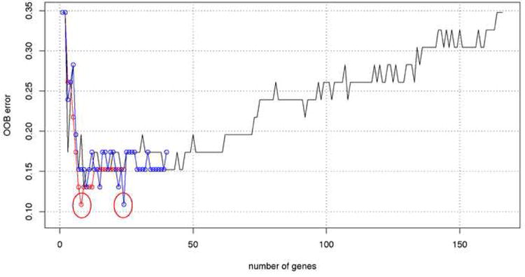
Change of OOB error rate with the number of genes selected by two methods importance and clustering ranking in one example run of the RF. The black line corresponds to genes selected by importance ranking of the initial 166 genes set. Blue circles represent 40 convergent genes ranked by the importance measure. Minimum error (11%) is obtained with k = 24 genes, circled in red. Red circles correspond to the error rate with k-best genes selected from k clusters (x axis). Minimum error (11%) is obtained with k = 8 genes, circled in red.

The procedure of gene selection was repeated 50 times. At each run we recorded the number of predictive genes obtained by importance and cluster-based ranking. Figure 3 shows the distribution of the number of genes obtained from the two methods in each of the 50 runs. A total of 13 best gene sets with minimal OOB error were constructed in these runs. The lowest OOB error rate was 11%. A set of 8 genes with the 11% error rate was selected 30 times by clustering and once by importance. The next best gene set with the same accuracy contained 12 genes and was selected 10 times by importance. These results indicate that a conclusion based on one run could be misleading since different runs resulted in a different number of genes with minimum error with both methods. Thus, the results from this procedure were combined to identify all of the best predictive transcripts. The combination of all predictive genes resulted in 24 gene transcripts. Using the gene predictive index defined in equation (3) we ranked the final list of transcripts. The results are given in the supplementary Table S1 with the 8 best predictor transcripts indicated at the top of the ranking.

Figure 3.

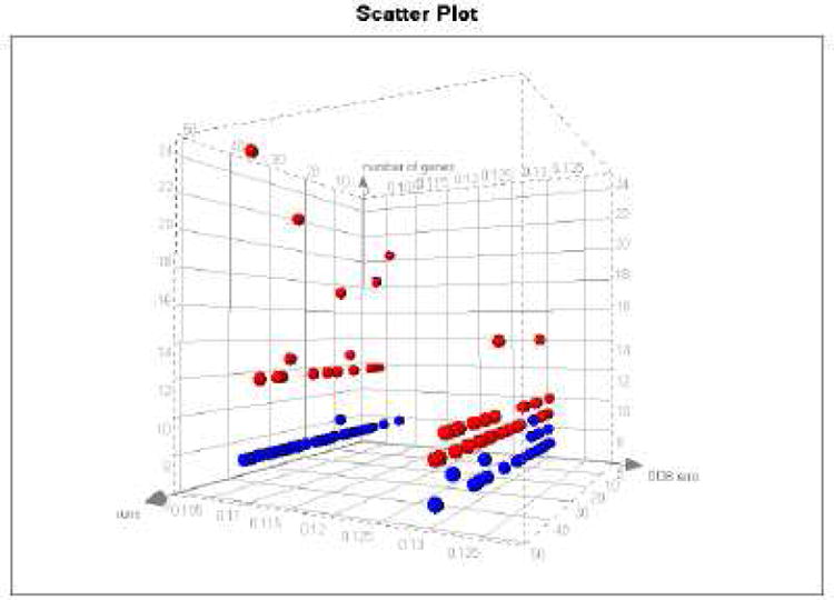
Number of genes (y axis) with minimum error (x axis) obtained by importance ranking (red) and clustering (blue) in 50 separate random forest runs (z axis).

As a final step, we ran RF starting from the first ranked gene (Table S1), then adding the second, third, and so on until we added the final ranked gene. Each time we recorded OOB error rate. As shown in supplementary Figure S5, the error rate levels off after the first 8 transcripts and the maximum accuracy (89%) is obtained with 8 top ranked transcripts, our best predictor. Among the 24 transcripts, 10 were selected by the clustering method and all were selected by the importance ranking. Overall the clustering selection is more consistent across iterations and selects fewer genes than importance ranking, 10 versus 24.

In Table 1 we compare the sensitivity and specificity of the two gene sets. The RF accuracy of the 24-gene set is slightly worse than the accuracy of the best 8-gene predictor but the difference is not significant given the sample size. We also checked that a predictor built using gene expression values estimated by the RMA method (we used the GCRMA initially) has the same accuracy (data not shown). The ultimate goal is the identification of the biomarker set that translates to a robust technology platform, such as Q-PCR, that could be used in a clinical setting. It has been shown that for most transcripts and probes designed to the same sequence regions Q-PCR measurements correlate well with hybridization measurements of expression (such as Affymetrix) [18; 19; 20]. Nevertheless one can expect that some probe design will fail among 24 transcripts and thus it is prudent to continue diagnostic development from this larger set of 24-genes while keeping focus on the 8-best genes.

Table 1.

Performance of the two best gene predictor sets. The prediction was done with the RF predictor and the accuracies were calculated with the OOB cross-validation. 95% confidence level intervals are included in parenthesis.

Gene set	Predicted	Non-responder	Responder
8-genes	NON-RESPONDER	20	2	Speci 91% (CI 69%-98%) Sens 88% (CI 67%-97%)
	RESPONDER	3	21
	Accuracy 89%	NPV 91% (CI 70%-98%)	PPV 87% (65%-97%)
24-genes	NON-RESPONDER	19	3	Spec 86% (CI 64%-96%) Sens 88% (CI 67%-97%)
	RESPONDER	3	21
	Accuracy 83%	NPV 86% (CI 64%-96%)	PPV 88% (CI 67%-97%)
BRASS Test set	NON-RESPONDER	1	0	Spec 100% (CI 5%-100%) Sens 90% (CI 54%-99%)
	RESPONDER	1	9
	Accuracy 83%	NPV 50% (CI 3%-97%)	PPV 100% (CI 63%-100%)

Comparison of RF with other classification methods

After a candidate gene set was determined, we then explored how those genes perform with different classification methods as listed in Materials and Methods. In leave-one-out cross-validation tests we compared the performance of the 8-gene, 24-gene and 40-gene sets using different classification methods. The error-rates for those gene sets and methods are shown in the supplementary Table S2. For the 8-gene set several classification methods reached accuracy greater than 85%, including neural nets, linear discriminant analysis and several variants of Support Vector Machines (SVMs). Linear kernel SVM learning achieved the same accuracy of 89% as the RF. The RF leave-one-out cross validation error is the same as the OOB error. The 24-gene set predictor built with two variants of SVM had the best accuracy of 91%, however given the small number of samples these differences are not significant. These results demonstrate that predictive accuracy of the selected genes does not dependent the specific learning approach, the RF, used to identify them.

We have applied the 8-gene predictor to an independent set of blood sample profiles provided by the Brigham and Women's Hospital Rheumatoid Arthritis Sequential Study (BRASS) registry of RA patients. From the BRASS registry we obtained a small set of patients, with no prior exposure to anti-TNF agents, for whom pre-treatment gene expression data and anti-TNF response after 12 weeks were available. This set consisted of 9 responsive and 2 non-responsive patients. The BRASS blood samples were collected at a different site and were processed with a slight different protocol than the ABCoN samples. For the purpose of classifying BRASS patients we transformed the log2 expression values of 8 genes into log2 expression ratios of 7 genes: CLTB, MXRA7, CXorf52, COL4A3BP, YIPF6, FAM44A and SFRS2, to PGK1 (one of the 8 genes) and constructed a predictor with the same accuracy of 89% as the log2 expression-based predictor. With the ratio-based predictor we predict correctly 9 of 9 responders and 1 of the 2 non-responders (see Table 1), thus having 91% accuracy on this independent sample set, similar as the OOB estimates. However, due to a small representation of non-responders in the test set the 95% confidence margins are very large.

Example II: Prediction of Breast Cancer Metastasis

For the second application of the CRF predictor algorithm we have chosen a data set first analyzed by van't Veer et al [12]. In the original paper, gene expression profiles of fresh frozen primary tumor samples from 78 breast cancer patients were analyzed. Patients were followed for more than 5 years and the tumor metastasis time was reported. Patients with time to metastasis shorter than 5 years (poor prognosis) were assigned to one group and patients with time to metastasis longer than 5 years were assigned to the second group. The goal of this initial investigation was to determine the utility of gene expression profiles as diagnostic tools for predicting future metastatic events. This initial analysis has lead to the development of the MAMMAPRINT diagnostic that was approved for clinical use in 2007 (Agendia™). The original investigation identified 70 gene transcripts that predicted progression to metastasis with 83% accuracy. The original work [12]validated the 70-gene predictor by testing on 19 tumor samples that were not used for training. Our goal in applying the CRF predictor to the van't Veer data set was to determine whether the CRF algorithm leads to identification of a smaller number of genes with the same or better accuracy as the original set.

The initial data processing (see Materials and Methods) identified 223 genes as candidates for building the predictor. The first step of the CRF approach selected the optimal RF parameters for this set. The optimal ntree value was at least 7510 trees while the optimal mtry=75. For simplicity we used 10,000 trees in the second step of the algorithm that identified genes consistently important for prediction. This step identified 103 different transcripts, and their identifiers and corresponding gene names are listed in the supplementary Table S3. The third step of the CRF algorithm identified and ranked the 30 best-predictive genes, which are listed in supplementary Table S4 with their predictive indexes. Eight of those genes are also in the original 70-gene set identified by van't Veer et. al [12]. As a final step of the process we built the predictor starting from the first gene ranked by GPI and added one gene at a time we found the best predictor. We found the best predictor to have only 8 transcripts with 86% accuracy of predicting progression to metastasis. Table 2 shows the performance of the 8 gene predictor on the training set of 78 samples as well as the test set of 19 samples. The accuracy of our 8-gene predictor, correctly predicting disease progression for 67 patients, is slightly better than the original 70-gene predictor. Additionally, the prediction accuracy of the 19 test case samples is equivalent to the training set, with 16 patients' disease progression predicted correctly.

Table 2.

Performance of the 8-gene RF predictor of poor or good metastasis prognosis. For the training set the accuracy was calculated with the OOB cross-validation. The predictor trained on the 78 samples was applied to 19 independent test samples. 95% confidence level intervals are included in parenthesis.

Sample set	Predicted	Poor prognosis	Good prognosis
training 78 samples	Poor prognosis	30	4	Specificity =88% (CI 72%-96%) Sensitivity =84% (CI 69%-93%)
	Good prognosis	7	37
	Overall accuracy is 86%	NPV = 81% (CI 64%-91)	PPV = 90% (CI 75%-97%)
testing 19 samples	Poor prognosis	11	1	Specificity =91% (CI 60%-100%) Sensitivity =71% (CI 30%-95%)
	Good prognosis	2	5
	Overall accuracy is 84%	NPV = 84% (CI 53%-97%)	PPV = 83% (CI 36%-99%)

Example III: Leukemia subtypes

We have also tested the CRF approach using the data set of 72 leukemia samples first analyzed by Golub et. al [21]. This set consists of two subtypes of leukemia: Acute Lymphocytic Leukemia (ALL) and Acute Myeloid Leukemia (AML). Gene expression data has been generated using one of the earliest versions of Affymetrix arrays profiling 7129 genes. As in the original publication we use for training the set of 38 samples (27 ALL and 11 AML) and for testing the independent set of 34 samples (20 ALL and 14 AML). The data has been preprocessed as described in Materials and Methods and 512 probe sets were identified as candidate biomarkers. The optimal ntree value for this data set was identified as 2155 trees and for simplicity we used 2200 trees for the next steps. Two optimal values of mtry were identified here mtry_O={8,18}. With these values the convergent step of CRF identified 80 consistently predictive transcripts that are listed in the supplementary Table S5. In the ranking and selection step 46 transcripts were identified and the top 8 transcripts on the list constitute the best predictor and are shown in supplementary Table S6. The 8-gene predictor has accuracy of 100% on the training set and 89% on the test set.

Example IV: Prostate cancer

One more data set that we have used for testing our method is a set of 52 prostate tumor and 50 normal prostate samples [22]. From this set we have selected randomly 40 tumor and 40 normal samples for training and used the remaining 12 tumor and 10 normal samples for testing as listed Materials and Methods. These expression profiles were generated using the hgu95a Affymetrix platform and represent 9,000 genes. The initial preprocessing of the data described in the Materials and Methods identified 921 gene transcripts as potential biomarkers. The parameter optimization steps of the CRF identified as optimal number of trees 1150, later on we use 1200 for simplicity. The optimal mtry_O ={51,54} for this dataset. The convergence step of the CRF identified 79 transcripts that are listed in Table S7. The ranking and final selection step identified 16 genes and the top 5 of those genes constitute the best predictor. The supplementary Table S8 lists the ranking of these 16 genes. The 5-gene predictor has an accuracy of 96% on the training set and 95% on the test set.

Comparison of the CRF and RSVM feature selection methods

Using all 4 data sets described above we have compared the CRF feature selection method and the recursive feature selection method implemented by Zhang et al called RSVM [15]. We selected RSVM as a representative of other recursive feature selection methods as it is readily available in R, an open source application, and has been shown to perform slightly better than other recursive methods [15]. Since CRF feature selection method is applied after the convergent set of genes are identified, we have applied the RSVM method to the set of genes identified after the convergence step: that is for the 40, 103, 80 and 79 genes identified for antiTNF response, BrCa metastasis, Leukemia and Prostate Cancer data sets. We have used for evaluation of classifiers' performance the area under curve measure (AUC) of the receiver operating characteristic (ROC). We used the BioConductor package ROCR [23] for these calculations. The selection of features by RSVM was implemented using the leave-one-out cross-validation error in the training set. In Table 3 we list the number of features selected by each method as well as the performance on the training and testing sets. The training set performance is calculated for OOB predictions of RF and leave-one-out cross-validation for the RSVM. Overall, the CRF method has a better performance than the RSVM method in all cases except the testing set of Leukemia subtypes where the AUC difference between the two methods is small, 0.036. The Leukemia set is the only case where the RSVM method reduced the convergent feature set from 80 to 60 genes, while in the other cases the RSVM did not identify a smaller number of predictive features. The feature selection by CRF always identifies much smaller number of genes than RSVM. For three of four data sets the CRF selected 8 genes and for the Prostate Cancer only 5. In all cases the performance estimated on the training set is almost the same as that for testing set. The largest difference between training and testing sets was for the anti-TNF response prediction where the testing set contains only two non-responders and nine responders.

Table 3.

Performance of the CRF and RSVM predictors evaluated by the AUC measure of performance. For the training set the performance of the CRF is estimated by the OOB error and for the RSVM by the leave-one-out cross-validation. The predictive features selected by each method are listed in the respective columns. Both methods selection was applied to the initial set of convergent genes.

Method	CRF				RSVM
Data Set	# convergent genes	Selected features	train AUC	test AUC	Selected features	train AUC	test AUC
Golub ALL AML	80	8	1.000	0.857	60	1.000	0.893
ProstateCancer	79	5	0.963	0.958	79	0.938	0.917
BrCaMetastasis	103	8	0.862	0.815	103	0.818	0.679
antTNF-response	40	8	0.890	0.750	40	0.828	0.500

Discussion

Different approaches have been developed for identification of biomarkers for disease classification, prediction of disease progression, and response to therapy. With genomic technologies one can measure a very large number of molecular features characterizing clinical samples. The identification of predictive biomarkers among thousands of features is the main challenge for data analysis. One challenge posed by the gene expression data is correlation of expression measurements across many genes. For samples that represent complex mixtures of cells, such as blood, the noise in expression data is not randomly distributed across the genes and samples. Thus the biomarker set representing several groups of correlated genes, where the noise is non-random, may be less accurate than a smaller set of un-correlated genes. While developing the Convergent Random Forest Predictor we followed the assumption that fewer genes will contain less noise and will lead to a more accurate predictor. Furthermore, identification of a small number of biomarkers would allow implementation of biomarker diagnostics using robust and sensitive technologies such as Q-PCR in contrast to less sensitive hybridization technologies used for large numbers of transcripts.

With respect to classifying patients, gene expression in tissue samples contains signal and noise. The signal may contain information about the patient's future response to therapy. The noise comes from several sources that may affect each gene differently but not necessarily in a random pattern. The conspicuous sources of noise are different genetic, dietary, health history and other patient backgrounds that are difficult to control or to take into account in the study design and data analysis. We thus expected that a set of few genes accumulates a smaller amount of noise relative to a large set and thus leads to the best predictor for drug response. Following this observation we have developed a CRF approach and applied it to identification of biomarkers of anti-TNF response in whole blood of Rheumatoid Arthritis patients. Additionally, we have shown validity of our approach to biomarker identification using 3 previously published data sets.

In the whole blood expression profiles of RA patients from the AbCoN initiative, the CRF algorithm identified 8 gene transcripts that predict response to anti-TNF treatment with 89% accuracy. The preliminary analysis of the gene expression data identified a subset of 166 genes as candidates for predictive genes. To refine the 166 informative genes into an accurate predictor, we followed several steps for feature identification and selection using the CRF approach. First, we searched for the optimal RF parameters to apply in our data. Second, using those optimal parameters, we implemented a converging RF algorithm that identified a smaller set of 40 transcripts with accuracy of 80%. Third, using gene expression clustering and gene importance determined by RF we developed a method for identifying the most predictive transcripts and introduced a Gene Predictive Index (GPI) for ranking transcripts. A final set of best predictors consists of 24 transcripts with an accuracy of 87%. With the GPI-based selection we further reduced the features to 8 genes that predict anti-TNF response with 89% accuracy. Similar accuracies are obtained for the selected gene sets with several distinct Machine Learning approaches. The accuracy of the predictor is also confirmed by an independent validation dataset of 11 patients from the BRASS registry however due to the small sample size and very uneven distribution of responders versus non-reponders the 95% confidence intervals on test set are very large. We note that with only 2- nonresponders calling everyone a responder would result in similar accuracy. Clearly, with just a small number of independent testing cases available to us at this time, the predictor validation requires a larger set of independent samples.

Given a small validation set for the anti-TNF case we more closely examine the issues that could lead to overfitting the 8-gene predictor. First our gene selection process is not cross-validated explicitly due to large computation time required for complete cross validation. However we addressed the overfitting problem by imposing very stringent False Discovery Rate (FDR) requirements for independent selection procedures. In the permutation and re-sampling procedure selecting genes correlated with DAS28 changes the FDR is 0.0005 (see Supplementary methods). In selection of genes differentially expressed in patients from healthy controls we use Bayesian posterior probabilities greater then 0.95. That results in selecting genes with p.value < 10^-6. Since we further require overlap between the differentially expressed genes and genes significantly correlated with DAS28 changes, our effective FDR is 10^-10 and with 166 genes selected there is very small likelihood (10^-8) that one is a false positive. Since each step of RF run is cross-validated this part of the procedure is cross-validated as well. A posteriori we confirmed that our 8-best genes are indeed significantly correlated with DAS28 changes in cross-validated permutation and resampling tests.

The twenty-four best genes identified by this analysis include genes known to be associated with rheumatoid arthritis or to have immune-related functions. Two of those genes are histone deacetylases HDAC4 and HDAC5. Histone deacetylase activities are required for innate immune cell control [24]. It has been also shown that histone deacetylase inhibition induces antigen specific anergy in lymphocytes [25] and regulates the induction of MHC II class genes [26]. Another gene, COL4A3BP (collagen, type IV, alpha-3 binding protein), has been identified as a protein binding the autoimmune Goodpasture syndrome autoantigen (COL4A3) [27]. COL4A3BP, also known as CERT kinase, phosphorylates the N-terminal region of COL4A3 and its elevated expression has been associated with immune complex mediated pathogenesis and increased IgA deposits in glomerular basement membrane [28]. We also identified as predictors other genes linked to immune responses, including MXRA7 and PGK1. Thus identification of several immune-related genes as features of the best predictor further supports the validity of our approach.

The identification of predictive biomarkers in whole blood collected from RA patients demonstrates feasibility of devising a diagnostic test assessing a patient's likelihood to benefit from anti-TNF therapy. Patients with rheumatoid arthritis (RA) are generally treated with Tumor Necrosis Factor (TNF)- α inhibitors as second-line therapy if an oral medication such as methotrexate (MTX) is not adequate to control the symptoms. If one anti-TNF therapy does not lead to adequate symptom control, the current standard of care dictates switching to one or more of the other approved anti-TNF agents, followed by other biologic agents. However, the no-response rate for the first anti-TNF agent is over 50% and increases for subsequent anti-TNF agents [29]. Clinical research indicates that the non-response to a second anti-TNF therapy closely correlates with the lack of response to the first one. Thus a diagnostic test performed before the initial anti-TNF therapy could save the patient from subsequent rounds of similar therapies that are likely to be ineffective but still can have serious side effects. The biomarker predictor identified in this investigation identifies the non-responders to therapy with ∼90% accuracy. If that level of accuracy is confirmed in a larger cohort, such a diagnostic would lead to changes in way RA is treated. Likely every patient will initially be treated an anti-TNF agent, but given a diagnostic prediction of non-response the patient could be directed to therapies with a different mechanism of action. Additionally the small number of biomarkers identified here would allow for implementation of the diagnostic using Q-PCR technology. In contrast to whole genome hybridization-based expression profiling, Q-PCR is more sensitive and robust. Recently a Q-PCR-based AlloMap^® from Expression Diagnostics (XDx), measuring gene expression in the peripheral blood mononuclear cells, has been approved for monitoring for rejection the heart transplant patients. Our investigation indicates that a similar diagnostic test can be developed for guiding the choice of therapy for RA patients.

We have shown the validity of CRF approach by applying it to three previously published data sets. In the well-studied data set of primary breast cancer tumors, the CRF algorithm identified 8-gene transcripts that predict progression to metastasis with 86% accuracy. This data set was investigated by the pioneering work of van't Veer et al. [12]. The original analysis of this data identified 70-genes that predicted metastasis with 83% accuracy on the training set of samples and a similar accuracy on a test set. The application of the CRF approach has identified in this data set a much smaller set of only 8 genes that predict metastasis with the accuracy of 86% for the training set and a similar accuracy for the test set. Several other gene sets predictive of progression to metastasis have been evaluated in the literature with a similar predictive power [30], including the 21-gene assay used by Oncotype DX, the alternative to the Mammaprint diagnostic. We note that our 8-gene set is also considerably smaller than the Oncotype DX diagnostic set. The 8-gene set has only one gene, MMP9, in common with the original 70-gene signature. However, the lack of a substantial overlap among gene sets does not mean that the classifier is not robust, as has been recently shown for the 70-gene, 21-gene and wound healing signatures applied to prediction of breast cancer progression [17].

The 8 genes selected as the best predictor of progression to metastasis are: MMP9, CA9, PIB5PA, NUP210, FBP1, IFITM1, SLC37A1 and TSPYL5. Among those eight genes two have been recently linked to the invasive (i.e. metastatic) breast cancer phonotype. It has been recently shown that up-regulation of several metalloproteinases (MMPs), including MMP9, is associated with the metastatic phenotype of breast cancer [31]. Additionally the up-regulation of the CA9 correlates with fast progression to metastasis [32].

We have demonstrated that the CRF approach, for selection of non-redundant molecular features predictive of a disease progression or treatment response, identifies the minimal number of features with a maximal predictive power. We note that once the non-redundant predictive features are identified, many of the machine learning approaches, such as SVMs and neural nets have predictive power similar to RF. We have compared the CRF and RSVM approach to feature selection. RSVM uses a recursive feature selection method representative of other recursive approaches. The comparison was performed on 4 very different sets of profiling data, each consisting of training and independent testing sets of samples. In each case only the testing set of samples were used for the identification of predictive features. Both methods constructed predictors with comparable performance as measured by the area under the ROC curve. Consistently the CRF identified much smaller number of features then RSVM, and had performance somewhat better for all but one testing set of data used for comparison. In any disease or therapy setting, the selection of just a few gene features would allow for a straightforward translation of the signature gene set discovered with genome-wide profiling, such as Affymetrix chips, to standard Q-PCR or sequencing technologies that have higher accuracy and lower costs. Thus we believe that the CRF method will help put into practice future molecular diagnostics that will assist in the implementation of individualized patient treatment.

Materials and Methods

Patient data

TNF-block response prediction

Patient blood samples were collected pre-treatment in PAXgene tubes. Whole blood RNA was extracted and profiled using standard protocols on Affymetrix hgu133plus2 chips. For details see Supplementary Materials and Methods. Rheumatoid Arthritis patients with active disease and naïve to TNF-blocking therapy were enlisted in the study. Response to TNF-blocking therapy was assessed after 14 weeks of treatment. Twenty-four patients were classified as responders and twenty-two as non-responders according to the EULAR classification [33; 34]. This data is available from the Gene Expression Omnibus (GEO) database at NCBI and has the accession number GSE15258.

Breast Cancer progression to metastasis

The patient population description can be found in the original paper [12] and the supplementary materials available from the web site http://www.rii.com/publications/default.html. Briefly, the training set consist of 78 samples with 34 samples belonging to patients with progression to metastasis after less than 5 years and 44 samples from patients with the onset of metastasis more than 5 years after the first diagnosis. The test set contains 19 samples with 12 patients progressing to metastasis within 5 years and 7 patients with less aggressive disease.

Leukemia data set

Data for the testing and training sets were downloaded from the Broad Institute Cancer Program site: http://www.broad.mit.edu/cgi-bin/cancer/datasets.cgi. Both molecular and patient data are available from the site.

Prostate Cancer data set

Data were downloaded from the Broad Institute Cancer Program site: http://www.broad.mit.edu/cgi-bin/cancer/datasets.cgi. We have randomly selected for testing the following samples: N11, N17, N20, N24, N25, N34, N35, N44, N59, N62, T05, T16, T17, T20, T21, T24, T28, T31, T36, T37, T38, T46,

Initial data processing for anti-TNF response prediction

Gene expression was analyzed starting with GCRMA normalization. Transcripts from the AbCoN training set was first reduced to those considered present in at least 50% in the samples from the same phenotypic group. Second, only transcripts that were significantly correlated with score for disease progression were selected. The significance was assessed using re-sampling and permutation as described in Supplementary Materials and Methods. Third only transcripts that were significantly different between responder, non-responder and healthy controls groups were considered. In the last and final step only transcripts with high expression and representing known genes in the ENTREZ database were selected. Details of this analysis are in Supplementary Materials and Methods. All analysis were done using the packages from R and Bioconductor [35].

Initial processing for breast cancer metastasis prediction

We have downloaded expression and clinical patient data from the website http://www.rii.com/publications/default.html. First a set of genes the are significantly different from the reference sample was selected as described in the original paper [12]. For the identification of the most relevant transcripts, the ratios of intensities were fitted the logistic regression model of the metastasis status. The significance of the fit was assessed by re-sampling and permutation tests similar to the ones applied to the anti-TNF data (see Supplementary Materials and Methods). This preprocessing selected 223 gene transcripts relevant to metastasis prediction. All calculations were done using R statistical programming language.

Initial processing of the Leukemia data set

This data set is available as normalized and background corrected intensities. All the negative intensity values were replaced by 1 and then data was log2 transformed. Using only the training set we have identified those transcripts that were present in at least 50% of the ALL or 50% of AML samples. This procedure identified 2231 transcripts. For the identification of the most relevant transcripts, the log2-trainsformed intensities were fitted the logistic regression model of ALL-AML status. The significance of the fit was assessed by re-sampling and permutation tests as are described for BrCa metastasis set in Supplementary Materials and Methods. This procedure identified 516 transcripts that are candidate biomarkers analyzed by the CRF method.

Initial processing of the Prostate Cancer data set

These data are available as the raw intensity CEL files. We normalized the data using the GCRMA procedure and using the MAS5 presence/absence calls identified genes present in at least 50% of the tumor or 50% of the normal samples. This step identified 1783 transcripts. For identification of the most relevant transcripts, the log2-transformed intensities were fitted the logistic regression model of tumor-normal status. The significance of the fit was assessed by re-sampling and permutation tests as are described for BrCa metastasis set in Supplementary Materials and Methods. This procedure identified 921 transcripts that are candidate biomarkers analyzed by the CRF method.

Other classification algorithms

The classification algorithms that were run in comparison to RF include. (1) k nearest neighbor classifier (kNN) is run with k ={1, 3, 5, …, 21} and k with the smallest error was chosen. (2) SVM [36] with radial kernel was run with combinations of cost parameter c ={1, 2, 4} and the parameter γ={2^-1/18, 1/18, 2/18} as suggested by Gentleman et al. [37]. Random forest was run with 10,000 trees and default mtry. The analysis was performed using MLInterfaces package in R. We have used the RSVM.R functions as provided by the authors on the web site http://www.stanford.edu/group/wonglab/RSVMpage/R-SVM.html.

The CRF method has been implemented in R and is available from authors upon request: Jadwiga.Bienkowska@biogenidec.com.

References

- 1.Guyon I, Weston J, Barnhill S, Vapnik V. Gene selection for cancer classification using support vector machines. Machine Learning. 2002;46:389–422. [Google Scholar]
- 2.Krishnapuram B, Carin L, Hartemink AJ. Joint classifier and feature optimization for comprehensive cancer diagnosis using gene expression data. Journal of Computational Biology. 2004;11:227–42. doi: 10.1089/1066527041410463. [DOI] [PubMed] [Google Scholar]
- 3.Golub TR, Slonim DK, Tamayo P, Huard C, Gaasenbeek M, Mesirov JP, Coller H, Loh ML, Downing JR, Caligiuri MA, Bloomfield CD, Lander ES. Molecular classification of cancer: class discovery and class prediction by gene expression monitoring. Science. 1999;286:531–7. doi: 10.1126/science.286.5439.531. [DOI] [PubMed] [Google Scholar]
- 4.Breiman L. Random forests. Machine Learning. 2001;45:5–32. [Google Scholar]
- 5.Enot DP, Beckmann M, Overy D, Draper J. Predicting interpretability of metabolome models based on behavior, putative identity, and biological relevance of explanatory signals. Proc Natl Acad Sci U S A. 2006;103:14865–70. doi: 10.1073/pnas.0605152103. [DOI] [PMC free article] [PubMed] [Google Scholar]
- 6.Gunther EC, Stone DJ, Gerwien RW, Bento P, Heyes MP. Prediction of clinical drug efficacy by classification of drug-induced genomic expression profiles in vitro. Proc Natl Acad Sci U S A. 2003;100:9608–13. doi: 10.1073/pnas.1632587100. [DOI] [PMC free article] [PubMed] [Google Scholar]
- 7.Mehrian-Shai R, Chen CD, Shi T, Horvath S, Nelson SF, Reichardt JKV, Sawyers CL. Insulin growth factor-binding protein 2 is a candidate biomarker for PTEN status and PI3K/Akt pathway activation in glioblastoma and prostate cancer. Proc Natl Acad Sci U S A. 2007;104:5563–68. doi: 10.1073/pnas.0609139104. [DOI] [PMC free article] [PubMed] [Google Scholar]
- 8.Seligson DB, Horvath S, Shi T, Yu H, Tze S, Grunstein M, Kurdistani SK. Global histone modification patterns predict risk of prostate cancer recurrence. Nature. 2005;435:1262–6. doi: 10.1038/nature03672. [DOI] [PubMed] [Google Scholar]
- 9.Shi T, Seligson D, Belldegrun AS, Palotie A, Horvath S. Tumor classification by tissue microarray profiling: random forest clustering applied to renal cell carcinoma. Modern Pathology. 2005;18:547–57. doi: 10.1038/modpathol.3800322. [DOI] [PubMed] [Google Scholar]
- 10.Liaw A, Wiener M. Classification and regression by randomForest. Rnews. 2002;2:18–22. [Google Scholar]
- 11.Breiman L. Random Forests. Machine Learning. 2001;45:5–32. [Google Scholar]
- 12.van't Veer LJ, Dai H, van de Vijver MJ, He YD, Hart AA, Mao M, Peterse HL, van der Kooy K, Marton MJ, Witteveen AT, Schreiber GJ, Kerkhoven RM, Roberts C, Linsley PS, Bernards R, Friend SH. Gene expression profiling predicts clinical outcome of breast cancer. Nature. 2002;415:530–6. doi: 10.1038/415530a. [DOI] [PubMed] [Google Scholar]
- 13.Díaz-Uriarte R, Alvarez de Andrés S. Gene selection and classification of microarray data using random forest. BMC Bioinformatics. 2006;7 doi: 10.1186/1471-2105-7-3. [DOI] [PMC free article] [PubMed] [Google Scholar]
- 14.Jiang H, Deng Y, Chen HS, Tao L, Sha Q, Chen J, Tsai CJ, Zhang S. Joint analysis of two microarray gene-expression data sets to select lung adenocarcinoma marker genes. BMC Bioinformatics. 2004;5 doi: 10.1186/1471-2105-5-81. [DOI] [PMC free article] [PubMed] [Google Scholar]
- 15.Zhang X, Lu X, Shi Q, Xu XQ, Leung HC, Harris LN, Iglehart JD, Miron A, Liu JS, Wong WH. Recursive SVM feature selection and sample classification for mass-spectrometry and microarray data. BMC Bioinformatics. 2006;1977 doi: 10.1186/1471-2105-7-197. [DOI] [PMC free article] [PubMed] [Google Scholar]
- 16.Ein-Dor L, Kela I, Getz G, Givol D, Domany E. Outcome signature genes in breast cancer: is there a unique set? Bioinformatics. 2005;21:171–8. doi: 10.1093/bioinformatics/bth469. [DOI] [PubMed] [Google Scholar]
- 17.Fan C, Oh DS, Wessels L, Weigelt B, Nuyten DS, Nobel AB, van't Veer LJ, Perou CM. Concordance among gene-expression-based predictors for breast cancer. N Engl J Med. 2006;355:560–9. doi: 10.1056/NEJMoa052933. [DOI] [PubMed] [Google Scholar]
- 18.Allaire NE, Rieder LE, Bienkowska J, Carulli JP. Experimental comparison and cross-validation of Affymetrix HT plate and cartridge array gene expression platforms. Genomics. doi: 10.1016/j.ygeno.2008.06.010. in press. [DOI] [PubMed] [Google Scholar]
- 19.Canales RD, Luo Y, Willey JC, Austermiller B, Barbacioru CC, Boysen C, Hunkapiller K, Jensen RV, Knight CR, Lee KY, Ma Y, Maqsodi B, Papallo A, Peters EH, Poulter K, Ruppel PL, Samaha RR, Shi L, Yang W, Zhang L, Goodsaid FM. Evaluation of DNA microarray results with quantitative gene expression platforms. Nat Biotechnol. 2006;24:1115–22. doi: 10.1038/nbt1236. [DOI] [PubMed] [Google Scholar]
- 20.Shi L, Reid LH, Jones WD, Shippy R, Warrington JA, Baker SC, Collins PJ, de Longueville F, Kawasaki ES, Lee KY, Luo Y, Sun YA, Willey JC, Setterquist RA, Fischer GM, Tong W, Dragan YP, Dix DJ, Frueh FW, Goodsaid FM, Herman D, Jensen RV, Johnson CD, Lobenhofer EK, Puri RK, Schrf U, Thierry-Mieg J, Wang C, Wilson M, Wolber PK, Zhang L, Amur S, Bao W, Barbacioru CC, Lucas AB, Bertholet V, Boysen C, Bromley B, Brown D, Brunner A, Canales R, Cao XM, Cebula TA, Chen JJ, Cheng J, Chu TM, Chudin E, Corson J, Corton JC, Croner LJ, Davies C, Davison TS, Delenstarr G, Deng X, Dorris D, Eklund AC, Fan XH, Fang H, Fulmer-Smentek S, Fuscoe JC, Gallagher K, Ge W, Guo L, Guo X, Hager J, Haje PK, Han J, Han T, Harbottle HC, Harris SC, Hatchwell E, Hauser CA, Hester S, Hong H, Hurban P, Jackson SA, Ji H, Knight CR, Kuo WP, LeClerc JE, Levy S, Li QZ, Liu C, Liu Y, Lombardi MJ, Ma Y, Magnuson SR, Maqsodi B, McDaniel T, Mei N, Myklebost O, Ning B, Novoradovskaya N, Orr MS, Osborn TW, Papallo A, Patterson TA, Perkins RG, Peters EH, Peterson R, et al. The MicroArray Quality Control (MAQC) project shows inter- and intraplatform reproducibility of gene expression measurements. Nat Biotechnol. 2006;24:1151–61. doi: 10.1038/nbt1239. [DOI] [PMC free article] [PubMed] [Google Scholar]
- 21.Golub TR, Slonim DK, Tamayo P, Huard C, Gaasenbeek M, Mesirov JP, Coller H, Loh ML, Downing JR, Caligiuri MA, Bloomfield CD, Lander ES. Molecular classification of cancer: class discovery and class prediction by gene expression monitoring. Science. 1999;286:531–7. doi: 10.1126/science.286.5439.531. [DOI] [PubMed] [Google Scholar]
- 22.Singh D, Febbo PG, Ross K, Jackson DG, Manola J, Ladd C, Tamayo P, Renshaw AA, D'Amico AV, Richie JP, Lander ES, Loda M, Kantoff PW, Golub TR, Sellers WR. Gene expression correlates of clinical prostate cancer behavior. Cancer Cell. 2002;1:203–9. doi: 10.1016/s1535-6108(02)00030-2. [DOI] [PubMed] [Google Scholar]
- 23.Sing T, Sander O, Beerenwinkel N, Lengauer T. ROCR: visualizing classifier performance in R. Bioinformatics. 2005;21:3940–1. doi: 10.1093/bioinformatics/bti623. [DOI] [PubMed] [Google Scholar]
- 24.Brogdon JL, Xu Y, Szabo SJ, An S, Buxton F, Cohen D, Huang Q. Histone deacetylase activities are required for innate immune cell control of Th1 but not Th2 effector cell function. Blood. 2007;109:1123–30. doi: 10.1182/blood-2006-04-019711. [DOI] [PubMed] [Google Scholar]
- 25.Edens RE, Dagtas S, Gilbert KM. Histone deacetylase inhibitors induce antigen specific anergy in lymphocytes: a comparative study. Int Immunopharmacol. 2006;6:1673–81. doi: 10.1016/j.intimp.2006.07.001. [DOI] [PubMed] [Google Scholar]
- 26.Gialitakis M, Kretsovali A, Spilianakis C, Kravariti L, Mages J, Hoffmann R, Hatzopoulos AK, Papamatheakis J. Coordinated changes of histone modifications and HDAC mobilization regulate the induction of MHC class II genes by Trichostatin A. Nucleic Acids Res. 2006;34:765–72. doi: 10.1093/nar/gkj462. [DOI] [PMC free article] [PubMed] [Google Scholar]
- 27.Raya A, Revert F, Navarro S, Saus J. Characterization of a novel type of serine/threonine kinase that specifically phosphorylates the human goodpasture antigen. J Biol Chem. 1999;274:12642–9. doi: 10.1074/jbc.274.18.12642. [DOI] [PubMed] [Google Scholar]
- 28.Revert F, Merino R, Monteagudo C, Macias J, Peydro A, Alcacer J, Muniesa P, Marquina R, Blanco M, Iglesias M, Revert-Ros F, Merino J, Saus J. Increased Goodpasture antigen-binding protein expression induces type IV collagen disorganization and deposit of immunoglobulin A in glomerular basement membrane. Am J Pathol. 2007;171:1419–30. doi: 10.2353/ajpath.2007.070205. [DOI] [PMC free article] [PubMed] [Google Scholar]
- 29.Karlsson JA, Kristensen LE, Kapetanovic MC, Gulfe A, Saxne T, Geborek P. Treatment response to a second or third TNF-inhibitor in RA: results from the South Swedish Arthritis Treatment Group Register. Rheumatology (Oxford) 2008;47:507–13. doi: 10.1093/rheumatology/ken034. [DOI] [PubMed] [Google Scholar]
- 30.Thomassen M, Tan Q, Eiriksdottir F, Bak M, Cold S, Kruse TA. Comparison of gene sets for expression profiling: prediction of metastasis from low-malignant breast cancer. Clin Cancer Res. 2007;13:5355–60. doi: 10.1158/1078-0432.CCR-07-0249. [DOI] [PubMed] [Google Scholar]
- 31.Rizki A, Weaver V, Lee S, Rozenberg G, Chin K, Myers C, Bascom J, Mott J, Semeiks J, Grate L, Mian I, Borowsky A, Jensen R, Idowu M, Chen F, Chen D, Petersen O, Gray J, Bissell M. A human breast cell model of preinvasive to invasive transition. Cancer Research. 2008;68:1378–87. doi: 10.1158/0008-5472.CAN-07-2225. [DOI] [PMC free article] [PubMed] [Google Scholar]
- 32.Trastour C, Benizri E, Ettore F, Ramaioli A, Chamorey E, Pouyssegur J, Berra E. HIF-1alpha and CA IX staining in invasive breast carcinomas: prognosis and treatment outcome. Int J Cancer. 2007;120:1451–8. doi: 10.1002/ijc.22436. [DOI] [PubMed] [Google Scholar]
- 33.Fransen J, van Riel PL. The Disease Activity Score and the EULAR response criteria. Clin Exp Rheumatol. 2005;23:S93–9. [PubMed] [Google Scholar]
- 34.van Gestel AM, Haagsma CJ, van Riel PL. Validation of rheumatoid arthritis improvement criteria that include simplified joint counts. Arthritis Rheum. 1998;41:1845–50. doi: 10.1002/1529-0131(199810)41:10<1845::AID-ART17>3.0.CO;2-K. [DOI] [PubMed] [Google Scholar]
- 35.Genetelman R, Carey J, Huber W, Irizarry R, Dudoit S. Bioinformatics and Computational Biology Solutions using R and Bioconductor. Springer; 2005. [Google Scholar]
- 36.Vapnik V. The Nature of Statistical Learning Theory. Springer-Verlag; 1995. [Google Scholar]
- 37.Gentleman R, Carey J, Huber W, Irizarry R, Dudoit S. Bioinformatics and Computational Biology Solutions using R and Bioconductor. Springer; New York: 2005. [Google Scholar]
Associated Data
This section collects any data citations, data availability statements, or supplementary materials included in this article.