Native Purification and Analysis of Long RNAs

Abstract

The purification and analysis of long noncoding RNAs (lncRNAs) in vitro is a challenge, particularly if one wants to preserve elements of functional structure. Here, we describe a method for purifying lncRNAs that preserves the cotranscriptionally derived structure. The protocol avoids the misfolding that can occur during denaturation–renaturation protocols, thus facilitating the folding of long RNAs to a native-like state. This method is simple and does not require addition of tags to the RNA or the use of affinity columns. LncRNAs purified using this type of native purification protocol are amenable to biochemical and biophysical analysis. Here, we describe how to study lncRNA global compaction in the presence of divalent ions at equilibrium using sedimentation velocity analytical ultracentrifugation and analytical size-exclusion chromatography as well as how to use these uniform RNA species to determine robust lncRNA secondary structure maps by chemical probing techniques like selective 2′-hydroxyl acylation analyzed by primer extension and dimethyl sulfate probing.

1. INTRODUCTION

Biochemical and biophysical studies on RNA molecules in vitro require that target molecules are synthesized and purified as homogeneous, functional species. For catalytic RNAs, enzymatic assays can confirm that the target molecules are correctly folded (Russell et al., 2002; Wan, Mitchell, & Russell, 2009). For noncatalytic RNAs, folding homogeneity needs to be assessed by nonenzymatic, biochemical, or biophysical assays (Woodson, 2011).

Traditionally, two folding procedures have been successfully used in biochemical and biophysical studies of large RNAs, such as group I and II introns, other ribozymes, riboswitches, signal recognition particle RNA, and tRNAs. The first approach involves heat denaturation and refolding of the RNA after in vitro transcription (Fedorova, Waldsich, & Pyle, 2007; Lomant & Fresco, 1975; Takamoto, He, Morris, Chance, & Brenowitz, 2002; Walstrum & Uhlenbeck, 1990; Zhang & Ferre-D’Amare, 2013), whereas the second approach consists of cotranscriptional folding without any denaturation step (Batey, 2014; Toor, Keating, Taylor, & Pyle, 2008). The latter method preserves the secondary and/or tertiary structure adopted by the RNA during transcription, which can be important considering that functional RNA structures are formed cotranscriptionally in vivo (Frieda & Block, 2012; Heilman-Miller & Woodson, 2003; Lai, Proctor, & Meyer, 2013).

Long noncoding RNAs (lncRNAs) are involved in a staggering diversity of fundamental cellular functions and they represent important subjects for ongoing research (Gutschner & Diederichs, 2012). Most lncRNAs do not have ribozyme activity, but they are essential in development, transcription, and epigenetic processes (Necsulea et al., 2014). These RNAs, which can reach tens of kilobases in length, appear to have encountered weaker evolutionary selection constraints than protein-coding genes, thus accumulating repetitive sequences (Derrien et al., 2012). LncRNAs are therefore challenging molecules for biophysical analysis because they can form alternative conformations in the absence of any structural constraint (Huthoff & Berkhout, 2002). Given these properties, cotranscriptional native purification may be particularly useful for lncRNA targets.

Here, we describe a native purification protocol that results in pure, homogeneous lncRNA preparations amenable for biochemical and biophysical studies. While other purification methods make use of affinity tags suitable to extract RNA from in vivo sources (Batey & Kieft, 2007; Said et al., 2009), our protocol does not necessarily require tags. The use of tags, generally added to the 3′ end of target RNAs, ensures capturing a homogeneous population of full-length molecules. In our method, we achieve a similar goal by using a T7 polymerase construct that rarely produces short abortive transcripts (Tang et al., 2014), and centrifugal filtration and size-exclusion chromatography (SEC) as final polishing steps in purification. Not using tags may simplify cloning design and avoid inclusion of nonnative sequences that may interfere with structure formation of the target RNA. However, if tags are useful for downstream applications, their inclusion is compatible with our protocol.

We additionally describe methods to study lncRNA folding based on sedimentation velocity analytical ultracentrifugation (SV-AUC), analytical SEC, and chemical probing. These analytical techniques are provided as examples, as many other techniques (such circular dichroism, small angle X-ray scattering, etc.) can be used to monitor homogeneity and oligomeric state of long RNAs (Behrouzi, Roh, Kilburn, Briber, & Woodson, 2012; Pan & Sosnick, 1997; Rambo & Tainer, 2010). SV-AUC and analytical SEC allow one to monitor global compaction of RNA preparations in the presence of divalent ions, under equilibrium conditions (Cole, Lary, Moody, & Laue, 2008; Mitra, 2014), and the equipment required is commonly available. Chemical probing facilitates the determination of lncRNA secondary structure (Athavale et al., 2013; Novikova, Hennelly, & Sanbonmatsu, 2012), and it also utilizes reagents that are available to most investigators. In this review, we describe protocols for selective 2′-hydroxyl acylation analyzed by primer extension (SHAPE) and dimethyl sulfate (DMS) chemical probing, as they have been applied for studying lncRNAs (Novikova et al., 2012; Watts et al., 2009). Again, these represent only a subset of available techniques for mapping RNA structure in solution. The SHAPE and DMS methods employ an electrophilic reagent that reacts selectively with flexible, accessible sites on ribonucleotides, facilitating detection of loops and other single-stranded regions within lncRNA molecules.

2. NATIVE PURIFICATION OF LONG NONCODING RNAs

In this section, we outline the procedures for transcription and purification of lncRNAs following nondenaturing methods. These protocols are based on those developed in our laboratory in recent years (Fedorova, Su, & Pyle, 2002; Fedorova et al., 2007; Marcia & Pyle, 2012; Toor et al., 2008), which have been modified and updated to fit the idiosyncrasies of large non-coding RNAs that range from one to several kilobases in length (up to 4 kb in our hands). The pipeline of the procedure includes the design of the construct, linearization of the DNA template and transcription of the RNA, digestion of DNA, enzyme proteolysis, buffer exchange, and finally, filtration and purification using SEC (Fig. 1A).

Figure 1.

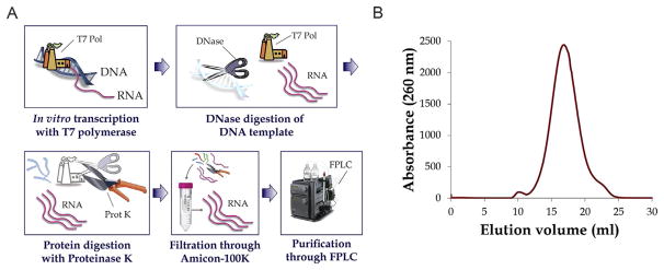
Enzymatic synthesis and purification of long noncoding RNAs. (A) The native purification pipeline of lncRNAs comprises the following steps (from left to right and top to bottom): the RNA is synthesized with the T7 RNA polymerase system; when the transcription reaction is finished, the DNA template is digested with DNase enzyme; enzymes in the reaction are then proteolyzed with the action of the proteinase K enzyme; RNA is captured from reaction components and buffer exchanged by ultra-filtration with Amicon centrifugal devices (Millipore); finally, the RNA is subjected to size-exclusion chromatography. (B) The resulting chromatogram represents the absorbance of the filtered RNA as a function of the elution volume. Material in the void volume of the column (10 ml elution) and shorter RNA molecules (22 ml elution) are excluded. The fraction(s) corresponding to the main peak are then selected for downstream analysis.

2.1 Construct design

The target lncRNA should be inserted into a suitable vector (e.g., pBluescript, Life Technologies) such that it is immediately flanked at the 5′ end by T7 promoter sequence and at the 3′ end by a unique and efficient restriction site (e.g., BamHI). In addition, we recommend digesting the template DNA with a restriction enzyme that produces blunt or 5′ overhanging ends to limit the production of heterogeneous RNA transcripts that vary in length (Schenborn & Mierendorf, 1985).

2.2 DNA plasmid linearization

1. Mix 50 μg of DNA plasmid with 80 U of the appropriate restriction enzyme in the presence of 1× restriction enzyme buffer in a final volume of 100 μl.

2. Incubate in a thermo block or mixer incubator at 37 °C overnight.

   Note: It is recommended to check that the plasmid is completely digested by running an agarose gel before starting the transcription reaction.

3. Purify the plasmid through phenol extraction followed by ethanol precipitation or through a spin column (Illustra MicroSpin G-25 column, GE Healthcare).

4. Quantify the concentration of the DNA template in a Nanodrop spectrophotometer (Thermo Scientific).

2.3 In vitro transcription of RNA

1. Prepare a transcription reaction in a final volume of 200 μl (Tables 1 and 2).

   1. We express our own batches of recombinant T7 RNA polymerase, which has a concentration of 2 mg/ml, approximately. We use the T7 RNA polymerase mutant P266L, which is known to produce short abortive transcripts less frequently than wild-type T7 polymerase (Tang et al., 2014). If using a commercial T7 RNA polymerase, we suggest following the manufacturer instructions.

   2. Scale up the reaction above according to the amount of RNA needed in subsequent steps. We have observed that the yield of the reaction varies among transcripts and factors affecting yield can include sequence (particularly in the first several nucleotides adjacent to the promoter), the length of the transcript, and the complexity of its secondary structure.

   3. It is also advisable to optimize the concentration of magnesium for each particular transcript. The concentration indicated in the table above corresponds to that optimized for lncRNA HOTAIR.

2. Incubate the reaction for 2 h at 37 °C in a thermo block or mixer incubator.

   1. Increasing the incubation time can result in increased RNA yields, although we do not recommend incubating longer than 4 h.

Table 1.

In vitro transcription reaction

Component	Final concentration	Stock	Amount
Transcription buffer (Table 2)	1×	10×	20 μl
DTT	10 mM	1 M	2 μl
ATP	3.6 mM	30 mM	24 μl
CTP	3.6 mM	30 mM	24 μl
GTP	3.6 mM	30 mM	24 μl
UTP	3.6 mM	30 mM	24 μl
RNaseOUT™	80 U	40 U/μl	2 μl
Pyrophosphatase	4 U	2 U/μl	2 μl
T7 polymerase	0.1 mg/ml	2 mg/ml	10 μl
Linearized plasmid	6.25 μg		31.25 ng/μl

Add deionized H₂O to 200 μl.

Table 2.

Transcription buffer (10×)

Component	Final concentration	Stock (M)	Amount (μl)
MgCl2	120 mM	1	120
Tris–HCl (pH 8.0)	400 mM	1	400
Spermidine	20 mM	2	10
NaCl	100 mM	5	20
Triton X-100	0.1%		1

Add deionized H₂O to 1 ml.

2.4 DNase digestion

1. After transcription, add 0.5 U of TURBO^™ DNase (2 U/μl) (Life Technologies) per microgram of DNA included in the transcription reaction, as recommended by the manufacturer.

   1. For the transcription reaction described above, we would typically include 1.5 μl of DNase; however, we often add more (2.5 μl).

   2. Note that DNase enzyme is sensitive to physical denaturation. Therefore, do not vortex the reaction mixture after addition of DNase.

2. Incubate at 37 °C for 30 min.

2.5 Proteinase K treatment

1. After the DNase treatment, add 2 μl of a 30 mg/ml stock of proteinase K powder (Life Technologies) dissolved in proteinase K storage buffer (Table 3) to proteolyze the enzymes present in the reaction mixture.

   1. According to manufacturer, a final concentration of 0.25 mg/ml (1.6 μl) of proteinase K is enough for the degradation of enzymes present in the reaction mixture. However, if the presence of proteinase K is not problematic for subsequent applications, we usually add an excess of enzyme.

2. Incubate at 37 °C for 30 min.

Table 3.

Proteinase K storage buffer (1×)

Component	Final concentration	Stock	Amount
Tris–HCl (pH 7.5)	10 mM	1 M	100 μl
CaCl2 (1 M)	1 mM	1 M	10 μl
Glycerol	40%	100%	4 ml

Add deionized H₂O to 10 ml.

2.6 EDTA chelation of divalent ions (optional)

In some cases, it is desirable to preserve all secondary and tertiary structure that is formed during transcription. In these cases, it is important to skip this step. However, if one wants to preserve secondary structural elements and eliminate tertiary structural features (e.g., for studies of RNA folding mechanism), then perform the chelation protocol described below.

After proteolytic digestion, divalent ions are chelated through the addition of EDTA to the solution. This treatment disrupts the RNA tertiary structure, but preserves stable secondary structure elements formed during the transcription reaction.

1. Add an amount of EDTA to the reaction that is equivalent to the number of divalent cations present in the transcription buffer.

   1. The reaction mixture described above contains 2400 nmol of MgCl₂. Therefore, add:

      $$2400\text{nmol}:500\text{nmol}/\mathrm{\mu }\mathrm{l}\text{of}\text{EDTA}=4.8\mathrm{\mu }\mathrm{l}\text{of}\text{EDTA}0.5M$$

2. Vortex briefly and spin down the tubes.

2.7 Buffer exchange and purification

Buffer exchange and separation of the RNA from enzymatic products is performed using commercially available Amicon^® Ultra Centrifugal Filters (Millipore) (http://www.emdmillipore.com/US/en/life-science-research/protein-sample-preparation/protein-concentration/amicon-ultra-centrifugal-filters/YKSb.qB.GXgAAAFBTrllvyxi,nav). This treatment allows the RNA to be equilibrated in filtration buffer (Table 4), a buffer solution containing physiological amounts of monovalent ions that preserve the secondary structure, while washing out unreacted nucleotides, digested DNA, protein fragments, and other components of the previous reactions.

Table 4.

Filtration buffer (1×)

Component	Final concentration (mM)	Stock (M)	Amount
MOPS buffer (pH 6.5)	8	1	4 ml
KCl	100	2	25 ml
EDTA (pH 8.5)	0.1	0.5	100 μl

Add deionized H₂O to 500 ml.

Short macromolecules, such as abortive transcription products and the proteinase K enzyme (18.5 kDa) are also generally filtered out, although the extent of the filtration depends on the cut-off of the Amicon filter selected. All the centrifugation steps should be carried out at room temperature. It is important to keep the RNA at room temperature at all times, since changes in temperature can trap RNA molecules in alternative conformations, decreasing the homogeneity of the sample. The size of the concentration device and the centrifugation conditions depend upon the final volume of the transcription reaction (Table 5).

Table 5.

Amicon-device centrifugation guide

Amicon filter	Txn volume (ml)	Rotor	Speed (rcf)	Time (min)
Amicon Ultra 0.5 ml	0.2–1	Fixed-angle rotor suitable for 2-ml tubes	4000	5×5 times
Amicon Ultra 15 ml	≥1	Swinging bucket rotor suitable for 50-ml tubes	3000	10–15

The Amicon^® Ultra Filters are manufactured in a range of molecular weight cut-offs (MWCO), which have been calibrated for globular proteins. We use those with a MWCO of 100 kDa for our lncRNAs, which range from 2 to 4 kb long, although the selected MWCO will vary according to the target of the study. In general, it is important to consider that selectivity of Amicon^® Ultra Filters is different for proteins and for RNAs. For example, a filter that retains globular proteins of a given molecular weight will retain RNA molecules that are six times smaller (Kim, McKenna, Viani Puglisi, & Puglisi, 2007).

2.8 Size-exclusion chromatography

SEC or gel filtration chromatography is used for native purification of the RNA in a homogenous form. Alternative conformations of the RNA that are induced by temperature fluctuations, multimeric forms of the RNA formed by self-complementarity and aggregation and prematurely terminated transcripts can be resolved by SEC without altering the native secondary structure of the lncRNA (Fig. 1B).

We use different bead size resins that we pack into a Tricorn 10/300 Empty High Performance Column (GE Healthcare) (CV of approximately 25 ml). The media are selected according to the size of the RNA, following GE Healthcare recommendations (http://www.gelifesciences.co.jp/catalog/pdf/18112419.pdf) (Table 6).

Table 6.

Selection of chromatography media and running conditions

RNA size (nt)	Media	Max. operating flow rate approx. (ml/min)	Max. operating back pressure (MPa)
1–200	Superdex 75	1	0.2
200–600	Superdex 200	1	0.2
600–2000	Sephacryl 400	1	0.2
1000–2000	Sephacryl 500	0.83	0.2
>2000	Sephacryl 1000	0.67	Not determined

All the procedures are carried out at room temperature, and empty columns should be packed at room temperature, following manufacturer recommendations (http://ge-catalog.campaignhosting.se/Documents/Tricorn/TricornInstructionsAC.pdf). We keep packed columns equilibrated with ddH₂O or 20% ethanol at 4 °C when they are not being used to avoid bacterial contamination. In addition, all filtration solutions and packed columns should be warmed up to room temperature before the run.

Use an appropriate fast protein liquid chromatography (FPLC) system (i.e., Akta FPLC, Akta Purifier, Akta Explorer, Akta Pure) equipped with wavelength detection at 260 nm. The system should be washed with an RNase decontamination solution like RNaseZap (Life Technologies) and the column washed with at least 3 column volumes (CV) of ddH₂O and equilibrated with 3 CV of filtration buffer.

The following steps should be performed during SEC of lncRNA:

1. Collect fractions of 0.5 ml volume. The homogeneity of the preparation will usually be apparent from the elution chromatogram (Fig. 1B). If the RNA of interest is homogenous and elutes as a single peak, this fraction should be collected.

   Note: Self-packed columns and RNA preparations usually lead to broader peaks than those generated by protein preparations that are run in commercially packed and calibrated columns.

2. Measure the concentration of each fraction using a Nanodrop spectrophotometer (Thermo Scientific) and record absorption value at 260 nm.

3. The fraction with the highest absorption should be used for further studies. If more material is necessary, neighboring fractions should be combined and the absorption value of the mixture recorded again.

At this point, the lncRNA is used for subsequent applications, like folding studies or secondary structure probing. If long-term storage is necessary, the preservation process should be validated to be proven that it does not affect RNA biochemical and biophysical properties (e.g., formation of nonspecific interactions, multimerization, structural rearrangements, precipitation, or degradation). Based on our experience, storage of long RNAs in cold impaired the reproducibility of our assays. For that reason, we work exclusively on freshly purified RNA.

3. STUDY OF THE RNA TERTIARY FOLDING BY SEDIMENTATION VELOCITY ANALYTICAL ULTRACENTRIFUGATION

In this section, we describe the preparation of the sample for an equilibrium SV-AUC assay, and we provide a brief description of the assembly of the analytical cells and the instrument, the ProteomeLab^™ XL-I analytical ultracentrifuge (Beckman Instruments). We also explain how to process the raw data in order to obtain the hydrodynamic parameters for a given RNA species. There are two basic parameters to consider when preparing an SV-AUC experiment:

The first parameter is the concentration of the sample. We typically determine the concentration of the RNA in terms of absorbance at 260 nm in the Nanodrop (Thermo Scientific). The range for maintaining a linear response is from 0.2 to 1.2 absorbance units. High sample concentrations are more prone to aggregation and can lead to artifacts; in addition, different preparations of RNA samples can vary in yield and using high concentrations of sample in every experiment reduces the number of assays that can be performed with the same RNA preparation. For these reasons, we recommend using the lowest concentration of RNA that provides a good signal. Generally, an absorbance of 0.2 at 260 nm is sufficient.

The second parameter is the rotor speed. This parameter needs to be adjusted based on the molecular weight and the expected hydrodynamic radius of the target molecule. We typically apply a speed ranging between 20,000 and 25,000 rpm for our lncRNAs. For further reference, Cole et al. (2008) provides a quick guide for selecting the rotor speed based on the molecular weight of the molecule (although the values he provides refer to globular proteins), and the estimated sedimentation coefficient of the particles, which can be assessed in a preliminary test.

3.1 Preparation of samples for a study of RNA folding

1. Take the fraction with the highest absorbance at 260 nm after the SEC step and write down the absorbance value.

2. Determine the number of samples that you can run by SV-AUC by dividing the absorbance value of the sample by the final absorbance value that you will use in the experiment, for example, 0.2. Following these recommendation, we usually have material to perform at least 12 titration measurements. If the concentration of the RNA sample is not enough for making the desired number of measurements, then mix several fractions. If there is insufficient material in the main fraction for your experiment, we recommend taking only the two fractions eluting immediately before and immediately after the peak.

3. Set up the folding reaction in a volume of 420–500 μl. Dilute the RNA up to the desired concentration (i.e., 0.2) and add 2× AUC buffer (Table 7).

4. For each titration point, you should prepare a blank control, which does not contain RNA. The blank control contains the same volume of filtration buffer than RNA sample and the same concentration of the other components (Table 8).

5. Incubate the folding reaction at 37 °C on a heat block for a period of time that allows the RNA to reach its equilibrium structure. We usually let the RNA equilibrate for 30 min to 1 h. At this point, the samples are ready to be loaded in the optical cells of the analytical ultracentrifuge.

Table 7.

AUC buffer (2×)

Component	Final concentration (mM)	Stock (M)	Amount
HEPES buffer (pH 7.4)	100	1	15 ml
KCl	400	2	30 ml
EDTA (pH 8.5)	0.2	0.5	60 μl

Add deionized H₂O to 150 ml.

Table 8.

Preparation of an SV-AUC experiment

B1	x μl filtration buffer 250 μl of 2 × AU buffer 100 μl of 5 × MgCl2 50 mM x μl water
S1	x μl RNA fraction num. X 250 μl of 2 × AU buffer 100 μl of 5 × MgCl2 50 mM x μl water

Example: 10 mM MgCl₂.

Vol_F = 500 μl.

3.2 Assembly of the optical cells, sample loading, and instrument setup

Each analytical cell consists of a centerpiece, two window assemblies, and a cell housing. We use the charcoal-filled Epon double-sector centerpiece by Beckman and sapphire windows because they are harder than quartz windows and so they have longer life. The cells are loaded into an An-60 Ti analytical rotor (Beckman Instruments).

1. Clean all components with RNaseZAP and distilled water, especially the centerpieces and the windows, which are in direct contact with the RNA sample.

2. Assemble the cells and the counterbalance following the manufacturer instructions (https://www.beckmancoulter.com/wsrportal/techdocs?docname=LXLA-TB-003).

3. Place the cell horizontally, facing the screw ring, and load 400 μl of blank sample in the left cavity and 380 μl of RNA-containing sample in the right cavity with a 500 μl Hamilton syringe. Repeat this procedure for the other two cells.

   Note: It is important that the meniscus of the blank sample is higher than that of the RNA sample so that it does not interfere with the data analysis (see Section 3.4).

4. Weigh the filled cells and make sure that opposing cells weigh within 0.5 g of each other.

5. Seal the filling holes with the red plug gaskets and screw the housing plugs in with a screwdriver.

6. Switch on the AUC instrument and place the rotor inside. Place the monochromator inside the ultracentrifuge as described by the manufacturer (https://www.beckmancoulter.com/wsrportal/techdocs?docname=LXLAI-IM-10). Activate the chamber vacuum by pressing the vacuum key on the instrument control panel.

   Note: The monochromator contains a blocking filter that can be used to eliminate wavelengths below 400 nm. For absorbance at 260 nm, position the monochromator blocking filter lever perpendicular to the stem.

3.3 Setting up a sedimentation velocity experiment

Here, we describe the parameters for a sedimentation velocity run of an lncRNA in the range of 2–3 kb in length. These parameters should be adapted for different targets under study, following sample concentration and rotor speed recommendations above to ensure complete sedimentation of the RNA molecules.

1. Open the ProteomeLab XL-A/XL-I User Interface Software (Beckman Instruments).

2. Click File>New File.

3. In the setup area, select the following values and options:

   1. Rotor: 4 hole

   2. Speed: 25,000 rpm

   3. Time: hold

   4. Temperature: 20 °C

   5. Type of scan: Velocity

   6. Optical system: Absorbance

   7. Use default values of R_min and R_max, and select 260 nm in the wavelength field.

   8. If you want to use the same scan settings for each cell, enter settings for Cell 1 and then click the All Settings Identical to Cell 1 box.

4. Click the Detail button and select the following options in the Velocity Detail dialog box:

   1. Replicates: 2

   2. Mode: Continuous

   3. Centerpiece: 2

   4. Accept the default values for the rest of the fields

5. In the setup area, click on Scan Options and select the following parameters:

   1. Leave all boxes unselected except for Stop XL after last scan.

   2. Select Overlay last 1 scan(s).

6. Click the Method button. Accept the default values in each field and select 100 scans in the number of scans field.

7. We usually perform a short- and low-speed method for the radial calibration of the instrument before performing the actual experiment. The following modifications to the setup parameters described above should be selected for the radial calibration run:

   1. In the setup area, change the following options:

      1. Speed: 3000 rpm

   2. Under Details, select the following options:

      1. Replicates: 1

   3. In Scan options, select the following box in addition to the previous ones:

      1. Radial calibration before first scan.

   4. In Method, select 1 scan.

8. Once the radial calibration is finished (around 7–10 min), let the sample stand inside the instrument for around 30 min to 1 h, to allow for temperature equilibration. After that, start the data acquisition with the Start Method Scan button.

9. When the run is complete, turn off the vacuum and take the monochromator and the rotor out. Remove the sample from the cells with a pipette and gel-loading tips and disassemble the optical cells. Clean them well with Beckman soap and distilled water, and place them back.

3.4 Data analysis

We use the software SEDFIT for data analysis (http://www.analyticalultracentrifugation.com/download.htm) (Schuck, 2000). SEDFIT is a method for size-distribution analysis that uses numerical solutions to the Lamm equations (Lebowitz, Lewis, & Schuck, 2002; Fig. 2A and B). SED-FIT also calculates hydrodynamic parameters like the Stokes radius (hydration radius) of the species sedimented in the presence of different concentrations of magnesium. The values of Stokes radius are then fit to the Hill equation and the value of the K_d or midpoint of the equilibrium folding transition is determined (Fig. 2C; Mitra, 2009, 2014).

Figure 2.

Study of the RNA tertiary folding by sedimentation velocity analytical ultracentrifugation (SV-AUC) and analytical size-exclusion chromatography (SEC). (A) Raw data from SV-AUC are analyzed using Sedfit program and the resulting fit is visualized using the GUSSI applet. (B) The sedimentation coefficient distribution is obtained for each magnesium titration point. The sedimentation coefficient of the main species increases as RNA is compacting in the presence of magnesium. The observed decrease in the absorbance at increasing magnesium concentrations is due to the hypochromicity effect, which occurs when RNA bases stack in the tertiary structure, thus diminishing its capacity to absorb ultraviolet light. (C) Stokes radii are calculated, represented as a function of magnesium concentration and fitted to the Hill equation. (D) Elution volumes in an analytical SEC experiment are plotted as a function of magnesium concentration. The hypochromicity effect is also observed as a decrease in the absorbance of the eluted RNA. At 50 mM magnesium chloride, the sample is mainly eluting in the void volume, which indicates that a nonspecific aggregation is occurring.

1. Click on Data and Load new files. Select all the data corresponding to one optical cell (RA1, RA2, or RA3). In the pop-up dialog, enter the loading interval, preferably 1, if the number of scans is not very high (around 100 is good).

2. In the main software interface, drag and drop the red line in the absorbance display to indicate tentatively the position of the sample meniscus, generally located at about 6 cm and the blue line to indicate the bottom of the cell, which is usually located at around 7.2 cm.

3. In the same view, drag and drop the green lines, which indicate the limits of the analysis. We recommend placing the left green line as close as possible to the red line, whereas we usually place the right green line at around 7 cm, to avoid including convection artifacts in the analysis.

4. In the Model dialog box, select Continuous c(s) with other prior knowledge and in the pull down dialog select Continuous c(s) Conformational Change Model. This model is useful when the molar mass of the main species is known and when this species undergoes a conformational change under the different ionic conditions. In this case, the main species will sediment with different s-values under the different magnesium concentrations.

5. Click on Parameters and enter the following data:

   1. The molar mass of the RNA under study.

   2. A tentative range of s-min and s-max to display the results.

   3. The resolution or number of data points of the analysis, which is generally left as default (100).

   4. The partial specific volume, which is approximately 0.53 ml/g for RNA molecules (Mitra, 2009).

   5. The buffer density and the buffer viscosity for the experimental conditions. We use the program SEDNTERP (http://sednterp.unh.edu/) to determine the density and viscosity of each buffer used in the magnesium titration. Select 20 °C under the Experiment tab and introduce the components of the buffer in the Solvent tab, under the Compute button (Table 9). Wherever needed, the values of density and viscosity for pure water are 0.99823 g/l and 0.01002 P, respectively.

   6. An initial value of 2 for the frictional coefficient is recommended.

   7. Start by selecting a confidence level of 0.7.

   8. Leave all boxes unchecked.

6. Click the Run command to get an initial assessment of the fit.

7. Some initial adjustment may be needed: modify the range of s-min and x-max that better fits the main peak observed. Take note of the sedimentation coefficient of the main species and use it to get a better estimation of the frictional coefficient of your RNA molecule in the Calculator included in SEDFIT software. Go to Options>Calculator>Calculate axial and frictional coefficient ratios. In the pop-up window, introduce the values required. Assume the partial specific volume and the hydration of the RNA molecule to be 0.53 ml/g and 0.59 g/g, respectively (Mitra, 2009).

8. In the Parameters tab, check the box meniscus to allow fitting of the estimated value. Click first on the Run command and then on the Fit command. Repeat these two commands assuming a confidence level of 0.95.

9. Go back to the Parameters tab and uncheck the meniscus box. Check the boxes Baseline, Fit Time Independent Noise, and Frictional Ratio. Indicate a confidence level of 0.7. Click on the Fit command to refine the model. Repeat the operation assuming a confidence level of 0.95.

10. Assess the quality of the fit by considering the rms deviation, which should be well below 0.01 and the Run test Z, which should have an upper limit of 30. A visual determination of the goodness of the fit can be observed by clicking Display>Subtract Calculated Ti noise From Raw Data or by running the plug-in GUSSI (http://biophysics.swmed.edu/MBR/software.html) and selecting Plot>GUSSI data-fit-residuals plot (Fig. 2A).

11. Document the fit and the parameters displayed in the SEDFIT window by storing a screenshot of the SEDFIT window. Copy the distribution table by selecting this option under the tab Copy (Fig. 2B).

12. Calculate the Stokes radius (R_H) of the RNA at each magnesium concentration. In SEDFIT go to Options>Calculator>Calculate axial and frictional coefficient ratios, and introduce the values corresponding to the RNA and the buffer at each titration condition. In the results window, take note of the value of the Stokes radius for each condition.

13. Represent the Stokes radii of the magnesium titration as a function of the magnesium concentration and fit the curve to a Hill equation using the software GraphPad Prism 6 (GraphPad Software):

    $$Y(R_{\mathrm{H}})=Y(H_{\mathrm{H},0})+(Y(R_{\mathrm{H},\mathrm{f}})-Y(R_{\mathrm{H},0}))\times \left(\frac{{[\text{Mg}]}^n}{K_{\text{Mg}}^n+{[\text{Mg}]}^n}\right),$$

    where R_H is the Stokes radius (in Å), R_H,f and R_H,0 are the Stokes radii for unfolded and folded RNA, which correspond to the titration point with the lower and the highest concentration of magnesium, respectively. K_Mg value is the concentration of magnesium at which 50% of the RNA is folded and n is the Hill coefficient, which indicates the cooperativity of the folding transition (Mitra, 2009; Su, Brenowitz, & Pyle, 2003; Fig. 2C).

Table 9.

Density and viscosity values of selected SV-AUC buffers as calculated by SEDNTERP

MgCl2 (mM)	Density (g/l)	Viscosity (P)
0	1.01157	0.01031
0.01	1.01167	0.01030
1	1.01168	0.01031
5	1.0119	0.01033
10	1.01223	0.01035
25	1.0133	0.01042

4. ANALYSIS OF THE RNA TERTIARY FOLDING BY ANALYTICAL SIZE-EXCLUSION CHROMATOGRAPHY

SEC can also be used as an analytical tool to observe global compaction of RNA molecules in the presence of divalent ions. The advantage of this approach lies in its ease of use and in the higher availability of necessary equipment. Specifically, we use the same chromatography system (Akta FPLC) (see Section 2.8.). In analytical SEC there is no need to collect fractions, although it is mandatory that the FPLC system is equipped with a UV cell to monitor absorbance of the RNA sample. A description of this technique is summarized below:

1. Purify the RNA following the procedures described in Section 2.

2. Set up a folding reaction as explained in Section 3.1. Test a broad range of magnesium concentrations to determine the upper limit at which the RNA is no longer compacting, but rather aggregating. This phenomenon is especially easy to detect in analytical SEC, since large aggregates of molecules elute in the void volume of the column (Fig. 2D).

3. For every magnesium concentration tested, the FPLC system must be equilibrated in the same buffer used for the folding of RNA. The equilibration is carried out with 1 CV of buffer, provided that the experiment is starting from the lower magnesium concentration, so that no residual magnesium interferes with the assay. In other cases, equilibration should be performed with 3 CV of buffer.

4. Inject the sample and run the same protocol as that used for the purification of the RNA (Section 2.8). Note that the UV cell of the Akta FPLC system is very sensitive and very low sample volumes can be used for an analytical SEC experiment. In particular, we load 3 μg of RNA per titration condition.

5. A typical elution profile that is representative of a titration experiment is shown in Fig. 2D. A shift in the elution volume at each titration point is indicative of the compaction of the RNA at increasing magnesium concentrations. Compared to an SV-AUC profile (Fig. 2B), the resolution of the shift and that of the decrease in absorbance due to the hypochromicity effect are lower. Nevertheless, analytical SEC offers a reliable method to evaluate homogeneity of the RNA at different magnesium concentrations and to detect aggregation and degradation events.

6. To compare elution profiles between different columns, we calculate the chromatographic partition coefficient, K_av, or distribution constant (Fig. 2D inset; Dai, Dubin, & Andersson, 1998):

   $$K_{\text{av}}=\frac{(V_{\mathrm{e}}-V_0)}{(V_{\mathrm{t}}-V_0)}$$

   where V_e is the RNA elution volume, V₀ is the void volume of the column, and V_t is the total volume of the column. In addition, the partition coefficient also provides a quantitative determination of the highest concentration of magnesium at which the RNA ceases to continue compacting. This value also represents the concentration of magnesium that is optimal to include in the folding step of subsequent biophysical and biochemical applications. In the case of HOTAIR lncRNA, we use 25 mM of magnesium (Fig. 2D inset).

5. DETERMINATION OF THE SECONDARY STRUCTURE OF LNCRNAS BY CHEMICAL PROBING

In this section, we will provide an approach for determining the secondary structure of an lncRNA by using two chemical probing techniques: SHAPE and DMS. It is important to note that chemical probing should be performed immediately after the purification step and the samples have to be kept at room temperature at all times, avoiding any cooling down or freezing step, as this promotes the rearrangement of RNA structures. We make use of automated, high-throughput capillary electrophoresis for the analysis of fragments generated after the primer extension reactions, which are carried out with fluorescent-coupled primers. The runs are performed in a campus-located facility (http://dna-analysis.research.yale.edu/), and the raw data are analyzed by either one the following software programs: ShapeFinder (Vasa, Guex, Wilkinson, Weeks, & Giddings, 2008) and QuShape (Karabiber, McGinnis, Favorov, & Weeks, 2013).

5.1 Designing and coupling of primers

Fluorescent-coupled primers are used for primer extension detection of modifications in the RNA. Primers should be designed following standard guidelines as for DNA sequencing (approximate length of 20 nucleotides, starting and ending with purine residues, and with an approximate GC content of 50%). In addition, G should be avoided at the 5′ end if possible, as it can quench fluorescence (Behlke, Huang, Bogh, Rose, & Devor, 2005). The primers should cover the full sequence of the target gene, spaced evenly every 200–220 nucleotides, approximately. Oligonucleotides are synthesized in 50 nmol scale and modified at the 5′ end with an amine group.

We use four spectrally different fluorescent dyes in the form of succinimidyl esters: 5-carboxy-X-rhodamine (5-ROX), 5-carboxyfluorescein (5-FAM), 6-carboxy-4′,5′-dichloro-2′,7′-dimethoxyfluorescein (6-FAM), and 6-carboxytetramethylrhodamine (6-TAMRA) (Anaspec). Succinimidyl esters (SE) are recommended because they form a very stable amide bond between the dye and the amine-modified oligonucleotide primer. SE dyes are hydrophobicand they are freshly dissolved in DMSO priorto thelabelingreaction. We have adapted the protocol for labeling amine-modified oligonucleotides from Life Technologies (http://tools.lifetechnologies.com/content/sfs/manuals/mp00143.pdf). A summary of the dye conjugation step is provided below:

1. Prepare a labeling reaction by mixing the amine-modified oligonucleotide with the dye (Table 10).

2. Incubate the reaction in the dark for 6 h to overnight at room temperature.

3. Ethanol precipitate the oligonucleotide to ensure removal of the free dye.

4. Purify the oligonucleotide in a denaturing 20% polyacrylamide gel.

5. Locate the labeled and unlabeled oligonucleotides by UV shadowing and cut out the labeled oligonucleotide.

6. Purify the oligonucleotide by the “crush-and-soak” method using 10 mM Tris (pH 8.0) and 300 mM NaCl and precipitate with ethanol. Oligonucleotides are finally dissolved in ddH₂O at a concentration of 20μM (stock) and 2 μM (working concentration).

Table 10.

Primer labeling reaction

Component	Final concentration	Stock	Amount (μl)
Oligonucleotide	440–660 ng/μl	4–6 mg/ml	11
SE-dye	2.52 μg/μl	18 mg/ml	14
Sodium tetraborate buffer (pH 8.5)a	75 mM	0.1 M	75

^aPrepare freshly before the coupling reaction or keep frozen aliquots at −20 °C.

5.2 Generation of sequencing ladders

Two sequencing ladder reactions are generated for assays to be analyzed by ShapeFinder and one or two for those to be analyzed by QuShape. In the first case, primers labeled with ROX and TAMRA are reserved for the sequencing ladders. In the second case, we usually prepare a single sequencing ladder with primers labeled with FAM. The nucleotide selected for the ladder varies with every target composition, and it is recommended to make ladder(s) complementary to the most frequent nucleotide(s). Here, we present an example for a ladder performed to detect the adenosines in the target sequence.

1. Combine the following amounts in an amber PCR tube:

   • 28.8 μl Master mix (Table 11)

   • 4μl Labeled primer 2 μM

2. Place each PCR tube, corresponding to each sequencing ladder, into a thermocycler and run a sequencing-ladder PCR program (Table 13).

3. Stop the reaction by adding 6.4 μl of stop mixture (Table 14).

4. At this point, mix both sequencing ladders if using two for the analysis. Add 196 μl of 100% ethanol and incubate at 4 °C for 5 min.

5. Spin at maximum speed for 30 min and wash two times with 70% ethanol.

6. Resuspend the pellet in 2 μl of water and 38 μl of formamide.

7. Store at −20 °C.

Table 11.

Sequencing-ladder master mix

Component	Final concentration	Stock	Amount (μl)
Plasmid template	1 ng/μl
Thermo sequenase buffer			1.84
ddTTP mixture (Table 12)			16
Thermo sequenase	0.25 U/μl	4 U/μl	1.84

Add deionized H₂O to 28.8 μl.

Table 13.

Sequencing-ladder PCR program

Number of cycles	Temperature (°C)	Time
1	96	1 min
25	96	20 s
	55	20 s
	72	1 min
1	72	5 min

Table 14.

Stop mixture

Component	Final concentration	Stock	Amount (μl)
Sodium acetate (pH 5.2)	1.5 M	3 M	200
Na-EDTA (pH 8.5)	0.05 M	0.1 M	200
Glycogen	0.8 mg/ml	20 mg/ml	16

Add deionized H₂O to 416 μl.

5.3 SHAPE reaction

The RNA purified following the procedure described in Section 2 is subjected to chemical modification using 1-methyl-7-nitroisatoic anhydride (1M7). We synthesize 1M7 in our laboratory following the protocol by Kevin Weeks and coworkers (Mortimer & Weeks, 2007), but there are other approaches and SHAPE reagents that can be employed, like NMIA and 1M6 (Rice, Leonard, & Weeks, 2014). The optimal amount of 1M7 should be titrated for every RNA target under study, since factors like the length of the molecule and the purity of each batch of reagent will influence the extent of the modification. As a starting point, use a final concentration of 1 mM 1M7 dissolved in DMSO.

1. Prepare the folding reaction (Table 15). Reactions are carried out in triplicate. For each replicate, prepare two tubes that will contain the folded RNA sample and one of the following: the reagent (1M7) for the (+) reagent sample or the solvent of the reagent (DMSO) for the (−) reagent sample. The latter sample will be used as a reference for the data analysis because it indicates reverse transcriptase (RT) stops that are not attributable to specific modifications of the 1M7 reagent in the molecule, but rather to RNA degradation or to premature termination of reverse transcription.

2. Fold the RNA by incubating at 37 °C for 45 min. The incubation time will vary depending on the target RNA.

3. Add 1M7 or DMSO to the tubes containing the folded RNA (Table 17).

4. Incubate the reaction at 37 °C for 5 min.

5. Add 320 μl of quench mixture (Table 18) and 1 volume of isopropanol.

6. After quenching the reaction mixture, samples are incubated on ice for an hour or overnight.

7. Spin the samples at maximum speed for 30 min and wash two times with 70% ethanol.

8. Dissolve the pellet in 50 μl of RNA storage buffer (Table 19) and proceed immediately with the primer extension analysis (Section 5.5) without freezing the samples.

Table 15.

Folding reaction

Component	Final amount/conc.	(+) Reagent sample (μl)	(−) Reagent sample (μl)
RNA	20 pmol
5 × monovalent mixture (Table 16)	1×	98	98
MgCl2 250 mM	25 mM	49	49

Add deionized H₂O to 490 μl.

Table 17.

SHAPE reaction

Component	Final amount/conc.	(+) Reagent sample	(−) Reagent sample
1M7 10 mM	1 mM	54.4 μl	–
DMSO		–	54.4 μl

Table 18.

Quench mixture

Component	Final concentration	Stock	Amount (μl)
Sodium acetate (pH 5.2)	1.5 M	3 M	200
Na-EDTA (pH 8.5)	0.05 M	0.1 M	200
Glycogen	0.8 mg/ml	20 mg/ml	16

Add deionized H₂O to 100 ml.

Table 19.

RNA storage buffer

Component	Final concentration (mM)	Stock (M)	Amount (μl)
MOPS (pH 6.5)	10	1	100
Na-EDTA (pH 8.5)	0.1	0.5	2

Add deionized H₂O to 10 ml.

5.4 DMS reaction

The second chemical modifier that we use in our laboratory for probing is DMS (Sigma-Aldrich, ≥99.8% purity). The stock of DMS is prepared by dissolving 5 μl of DMS in 645 μl of cold 100% ethanol (81.3 mM). The final concentration of DMS in reaction has to be titrated for each target RNA molecule, usually ranging from 1 to 15 mM. Here, we describe a DMS probing reaction optimized for HOTAIR lncRNA.

1. The folding reaction takes place using the same volumes as the SHAPE reaction. However, HEPES buffer reacts with DMS and so we use cacodylate buffer in the 5× monovalent ion mixture (Table 20).

2. Prepare a DMS reaction (Table 21).

3. Incubate the reaction at room temperature for 10 min.

4. Stop the reaction by adding 54.4 μl of quench mixture (Table 22).

5. Precipitate the RNA (Table 23).

6. Spin at maximum speed for 30 min and wash two times with 70% ethanol.

7. Resuspend the pellet in 50 μl of RNA storage buffer (Table 19).

8. Store at −80 °C or use in the primer extension reaction.

Table 20.

Monovalent ion mixture (5×)

Component	Final concentration	Stock	Amount (ml)
KCl	1 M	2 M	50
Cacodylic buffer (pH 7.0)	0.125 M	0.25 M	25
Na-EDTA (pH 8.5)	0.5 mM	100 mM	0.5

Add deionized H₂O to 100 ml.

Table 21.

DMS reaction

Component	Final amount/conc.	(+) Reagent sample	(−) Reagent sample
DMS 81.3 mM	8.13 mM	54.4 μl	–
Ethanol		–	54.4 μl

Table 22.

Quench mixture

Component	Final concentration	Stock	Amount
2-Mercaptoethanol	715 mM	14.3 M	50 μl

Add deionized H₂O to 1 ml.

Table 23.

Precipitation reaction

Component	Final concentration	Stock	Amount (μl)
Sodium acetate (pH 5.2)	50.6 mM	3 M	20
Na-EDTA (pH 8.5)	8.4 mM	0.5 M	20
Glycogen	8.4 μg/μl	20 mg/ml	0.5
Isopropanol			600

5.5 Primer extension reaction

The primer extension reaction is performed using the Superscript III RT (Life Technologies) to detect the specific stops of the enzyme due to the modifications in the RNA. The primers used in the reaction are labeled with fluorescent dyes. For experiments that will be analyzed with ShapeFinder, two different dyes, JOE and FAM, are used for the (+) and (−) reagent samples, respectively. For experiments that will be analyzed with QuShape, we use the same labeled primer for the reagent and the blank sample, in this case JOE because the samples will be loaded in different wells (see Section 5.8.). Here, we show an example where the (+) and the (−) reagent samples will be reverse transcribed using primers labeled with JOE and FAM.

1. Prepare an annealing reaction in amber Eppendorf tubes, protected from light (Table 24).

2. Heat the mixture at 95 °C for 2 min and then place the tubes on ice for 5 min. Incubate at 48 °C for 2 min.

3. Add 8 μl of RT mixture (Table 25) and incubate at 48 °C for 45 min.

4. Stop the reaction by adding 30 μl of the stop mixture (Table 26).

5. Precipitate by adding 1 volume (50 μl) of isopropanol.

6. At this moment, the reagent and the blank samples that have been reverse transcribed with different fluorophore-labeled primers are combined together (only for the data analysis in ShapeFinder). If the reagent and the blank samples are reverse transcribed with the same fluorophore-labeled primer (for the data analysis in QuShape), they are not combined.

7. Spin at maximum speed for 30 min and wash two times with ethanol 70%.

8. Resuspend the pellet in 2 μl of deionized water and 48 μl of deionized formamide. Dissolve pellet by heating at 65 °C for 2 min.

Table 24.

Annealing reaction

Component	Final amount/ conc.	(+) Reagent sample (μl)	(−) Reagent sample (μl)
RNA	1 pmol	x	x
2 μM labeled primer (JOE)	0.1 μM	1	3
2 μM labeled primer (FAM)	0.1 μM	–	1
2 mM Na-EDTA (pH 8.5)	0.1 mM	1	1
5 M betaine	1 M	4	4

Add deionized H₂O to 12 μl.

Table 25.

Reverse transcriptase (RT) mixture

Component	Final concentration	Stock	Amount (μl)
RT buffer	2.5×	5×	96
DTT	12.6 mM	100 mM	24
Betaine	944 mM	5 M	36
dNTP mix	1.26 mM	10 mM	24
Superscript III RT	10 U/μl	200 U/μl	9.6
Deionized H2O			1

Table 26.

Stop mixture

Component	Final concentration	Stock	Amount (μl)
Sodium acetate (pH 5.2)	1.3 M	3 M	800
Na-EDTA (pH 8.5)	11 mM	100 mM	200
Glycogen	110 μg/μl	20 mg/ml	10
Deionized H2O			800

5.6 Reactions for mobility shift correction

A mobility shift correction must be performed manually during data analysis with ShapeFinder for each primer set because the dyes alter the electrophoretic migration rates, and therefore cDNAs of the same length may have slightly different elution times. To generate a file for mobility shift correction, we prepare sequencing ladders as described in Section 5.2. The sequencing ladder reactions for mobility shift correction are performed with all the different labeled primers on the same DNA template and with the same type of ddNTP. Once primer extension reactions are complete, all the reactions with the different fluorophores are mixed and precipitated together, following the protocol described in Section 5.2. The pellet obtained is resuspended in 2 μl water and 38 μl formamide and dissolved at 65 °C in a heat block for 2 min. Note that if you change capillary electrophoresis conditions, a new mobility shift correction will be necessary. To avoid it, we recommend keeping the settings of the capillary instruments fixed.

5.7 Spectral calibration of the instrument

Before the first run on the instrument, a spectral calibration should be carried out with the dye set. A spectral calibration creates a matrix that corrects for the overlapping fluorescence emission spectra of the dyes used for coupling the primers. We calibrate an Applied Biosystems 3730×l DNA Genetic Analyzer for using it with the Applied Biosystems four-dye chemistry DS-20 Dye Set (5-FAM, JOE, TAMRA, ROX) (A filter set). The calibration standard is prepared as previously described (Watts et al., 2009). Briefly, four primer extension reactions are performed from primers labeled with the chosen dye set and located in different regions of a linearized control plasmid, so that four fluorescent cDNA fragments of different length are generated. The resultant primer extensions are then mixed together to obtain similar fluorescence intensity for all four dyes and loaded in the plate:

1. Linearize a pUC18 plasmid with restriction enzyme HindIII.

2. Label four primers complementary to pUC18 plasmid (Table 27) with the set of dyes used to calibrate the instrument, following the instructions in Section 5.1.

3. Prepare a PCR reaction for each labeled primer (Table 28).

4. Place the tubes in a thermocycler and run the spectral-calibration PCR program (Table 29).

5. Stop the primer extension reaction by adding 8 μl of stop mixture per reaction (Table 30).

6. Add 120 μl of 100% ethanol per primer extension reaction.

7. Spin at maximum speed for 30 min and wash with 70% ethanol.

8. Dissolve each pellet in 20 μl of deionized formamide and mix the four reactions together.

Table 27.

Primers used for spectral calibration

Primera	Dye	Fragment (nt)
CAGAGCAGATTGTACTGAGAG	5-FAM	242
GTGTGAAATACCGCACAGAT	6-JOE	206
GCGTAAGGAGAAAATACCGCATC	6-TAMRA	188
CGCCATTCGCCATTCAGGCTGCGCAACTG	5-ROX	155

^aWatts et al. (2009).

Table 28.

Spectral-calibration PCR reaction

Component	Final concentration	Stock	Amount (μl)
Linearized pUC18 plasmid	0.1 ng/μl	0.2 ng/μl	0.5
Thermo sequenase buffer	1×	10×	4
dNTP mixture	75 μM	0.75 mM	4
Labeled primer	0.0125 pmol/μl	2 μM	5
Thermo sequenase	0.16 U/μl	4 U/μl	1.6

Add deionized H₂O to 40 μl.

Table 29.

Spectral-calibration PCR program

Number of cycles	Temperature (°C)	Time
1	96	2 min
25	96	20 s
	55	20 s
	72	1 min
1	72	10 min

Table 30.

Stop mixture

Component	Final concentration	Stock	Amount (μl)
Sodium acetate (pH 5.2)	1.5 M	3 M	100
Na-EDTA (pH 8.5)	0.25 mM	0.5 M	100
Glycogen	10 mg/ml	20 mg/ml	10

5.8 Preparation of samples for capillary electrophoresis

Samples are mixed with deionized formamide and loaded in a 96-well plate according to the following guidelines, which can be modified to adjust the output signal:

1. Plates prepared for data analysis with ShapeFinder contain the (+) and the (−) reagent sample mix, together with the sequencing ladder mix, in a single well for every primer extension reaction that is carried out (Table 31).

2. Plates prepared for data analysis on QuShape contain the (+) reagent sample and a single sequencing ladder in one well whereas the (−) reagent sample and the same sequencing ladder are loaded in a different well. The advantage of this setup is that it allows the use of only two dyes (Table 32).

3. Mobility shift reactions are loaded in the same plate (Table 33).

4. Capillary electrophoresis is performed using an Applied Biosystems 3730×l DNA Genetic Analyzer with 96 capillaries equipped with a 50-cm capillary array (DNA Analysis Facility at Science Hill, Yale University). Runs were performed while maintaining an oven temperature of 63 °C and a run voltage of 15 kV. The instrument was prerun for 180 s before injecting the sample at 1.2 kV for 16 s. Note that very high signal should be avoided as signal cross-talk can occur despite proper spectral precalibration of the instrument.

Table 31.

Capillary electrophoresis sample preparation (ShapeFinder)

Component	Amount (μl)
Reagent/blank mix	7
Sequencing ladder mix	2
Deionized formamide	12

Table 32.

Capillary electrophoresis sample preparation (QuShape)

Component	Amount (μl)
Reagent or blank sample	7
Sequencing ladder	2
Deionized formamide	12

Table 33.

Mobility shift sample preparation

Component	Amount (μl)
Mobility shift reaction	5
Deionized formamide	15

5.9 Data analysis

The analysis of chemical probing data consists of the following steps: (i) processing of the capillary electrophoresis electropherograms to determine the absolute reactivities for each reaction, (ii) normalization of the reactivities, and (iii) use of the reactivity profiles obtained as constraints in a software program to deduce a secondary structure of the molecule (Fig. 3).

Figure 3.

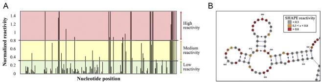
Determination of the secondary structure of lncRNAs by chemical probing. (A) After quantifying the absolute reactivity at each nucleotide position, SHAPE and DMS data is normalized on a scale spanning 0 to 2, approximately. Values lower than 0.3 represent constrained positions, which are part of double-stranded regions of tertiary interactions; values higher than 0.8 represent single-stranded regions; and values between 0.3 and 0.8 are likely single stranded. (B) Normalized reactivity values are used as constraints for RNA secondary structure prediction in RNAStructure software. In the figure, resulting secondary structure values are represented using VARNA software.

5.9.1 Determination of chemical probing reactivity profiles

The determination of chemical probing reactivity profiles can be carried out using either ShapeFinder (Vasa et al., 2008) or QuShape (Karabiber et al., 2013) software. We have used both of them successfully in our laboratory. The first one has been more extensively used, although it is no longer available online for download. The second one has been released more recently; it offers enhanced flexibility for utilizing multiple different fluorophores and it does not require import of mobility shift correction files. Regardless of the software used, the output containing the absolute nucleotide reactivity of the RNA sequence is presented as a file containing the calculated peak areas as a function of nucleotide position for the entire analyzed trace.

5.9.2 Normalization of SHAPE and DMS reactivity profiles

We normalize SHAPE and DMS data to a scale in which values ranging from 0 to 0.3 are considered not reactive; from 0.3 to 0.8, moderately reactive; and higher than 0.8, very reactive (Fig. 3A). It is important to note that the DMS reagent has different affinities for adenosine and cytosine residues and so the normalization of their reactivity profiles has to be done separately. The method described below has been modified from that previously reported by McGinnis, Duncan, and Weeks (2009):

1. Open the tab-delimited text file generated after alignment and integration in Microsoft Excel.

2. Calculate the third quartile value for the RX.area-BG.area column using the Excel function “=QUARTILE(array,quart),” where array is the cell range of numeric values for which you want the quartile value and quart is a number (3 represents the third quartile).

3. Copy the RX.area-BG.area column to a new spreadsheet and order the values in increasing order. Copy to a new column all values that fall in the range of ±10% of the third quartile value.

4. Calculate the average “=AVERAGE(number1, [number2]…)” of this new range of values.

5. Calculate and store the effective maximum reactivity value using the formula “=1.5*(AVERAGE(number1, [number2]…)),” where the range is represented by the values calculated in the point 4.

6. Divide the unsorted (RX.area-BG.area) of each nucleotide by the effective maximum reactivity value to obtain the normalized reactivity values. Values greater than this value are considered outliers and are excluded.

7. Create a new text file comprising two columns: the nucleotide numbers at the left and the normalized reactivity values at the right.

8. Combine all the text files with the normalized reactivity values from all the fragments corresponding to the same RNA.

In our laboratory, we have developed a modification of this method when performing side-by-side comparisons of a wild-type lncRNA and several mutants derived of the same lncRNA. In those cases, we have observed several consistent RT stops in all molecules, independently of the mutant, in both the (+) and (−) reagent samples. This observation is likely due to the inherent flexibility of some positions for each particular type of target RNA. In those cases, our normalization protocol excludes the (−) reagent sample and compares exclusively the (+) reagent samples, thus significantly reducing the observed error in the replicates.

5.9.3 RNA secondary structure prediction and analysis

The normalized reactivity values obtained are used as constraints for the secondary structure prediction of the RNA target using the RNAStructure software (Mathews, 2014; Reuter & Mathews, 2010). The software is available as a Web server or as a program with a graphical user interface, although we prefer the second option to avoid the sequence length restraints of using the Web server. Subsequently, RNA secondary structure coordinates can be visualized and modified using the Java applet VARNA (Darty, Denise, & Ponty, 2009). Additional editing can be also performed with Adobe Illustrator (Adobe Systems) or similar editor for vector graphics.

Table 12.

ddTTP mixture

Component	Final concentration (μM)	Stock (mM)	Amount (μl)
dATP	150	100	1.5
dCTP	150	100	1.5
dGTP	150	100	1.5
dTTP	150	100	1.5
ddTTP	1.5	1	1.5

Add deionized H₂O to 1 ml.

Table 16.

Monovalent mixture (5×)

Component	Final concentration	Stock	Amount (ml)
KCl	1 M	2 M	50
HEPES (pH 7.4)	0.25 M	1 M	25
Na-EDTA (pH 8.5)	0.5 mM	100 mM	0.5

Add deionized H₂O to 100 ml.

References

- Athavale SS, Gossett JJ, Bowman JC, Hud NV, Williams LD, Harvey SC. In vitro secondary structure of the genomic RNA of satellite tobacco mosaic virus. PLoS One. 2013;8:e54384. doi: 10.1371/journal.pone.0054384. [DOI] [PMC free article] [PubMed] [Google Scholar]
- Batey RT. Advances in methods for native expression and purification of RNA for structural studies. Current Opinion in Structural Biology. 2014;26:1–8. doi: 10.1016/j.sbi.2014.01.014. [DOI] [PMC free article] [PubMed] [Google Scholar]
- Batey RT, Kieft JS. Improved native affinity purification of RNA. RNA. 2007;13:1384–1389. doi: 10.1261/rna.528007. [DOI] [PMC free article] [PubMed] [Google Scholar]
- Behlke MA, Huang L, Bogh L, Rose S, Devor EJ. Fluorescence quenching by proximal G-bases. Integrated DNA Technologies; 2005. [Google Scholar]
- Behrouzi R, Roh JH, Kilburn D, Briber RM, Woodson SA. Cooperative tertiary interaction network guides RNA folding. Cell. 2012;149:348–357. doi: 10.1016/j.cell.2012.01.057. [DOI] [PMC free article] [PubMed] [Google Scholar]
- Cole JL, Lary JW, Moody TP, Laue TM. Analytical ultracentrifugation: Sedimentation velocity and sedimentation equilibrium. Methods in Cell Biology. 2008;84:143–179. doi: 10.1016/S0091-679X(07)84006-4. [DOI] [PMC free article] [PubMed] [Google Scholar]
- Dai H, Dubin P, Andersson T. Permeation of small molecules in aqueous size-exclusion chromatography vis-a-vis models for separation. Analytical Chemistry. 1998;70:1576–1580. [Google Scholar]
- Darty K, Denise A, Ponty Y. VARNA: Interactive drawing and editing of the RNA secondary structure. Bioinformatics. 2009;25:1974–1975. doi: 10.1093/bioinformatics/btp250. [DOI] [PMC free article] [PubMed] [Google Scholar]
- Derrien T, Johnson R, Bussotti G, Tanzer A, Djebali S, Tilgner H, et al. The GENCODE v7 catalog of human long noncoding RNAs: Analysis of their gene structure, evolution, and expression. Genome Research. 2012;22:1775–1789. doi: 10.1101/gr.132159.111. [DOI] [PMC free article] [PubMed] [Google Scholar]
- Fedorova O, Su LJ, Pyle AM. Group II introns: Highly specific endonucleases with modular structures and diverse catalytic functions. Methods. 2002;28:323–335. doi: 10.1016/s1046-2023(02)00239-6. [DOI] [PubMed] [Google Scholar]
- Fedorova O, Waldsich C, Pyle AM. Group II intron folding under near-physiological conditions: Collapsing to the near-native state. Journal of Molecular Biology. 2007;366:1099–1114. doi: 10.1016/j.jmb.2006.12.003. [DOI] [PMC free article] [PubMed] [Google Scholar]
- Frieda KL, Block SM. Direct observation of cotranscriptional folding in an adenine riboswitch. Science. 2012;338:397–400. doi: 10.1126/science.1225722. [DOI] [PMC free article] [PubMed] [Google Scholar]
- Gutschner T, Diederichs S. The hallmarks of cancer: A long non-coding RNA point of view. RNA Biology. 2012;9:703–719. doi: 10.4161/rna.20481. [DOI] [PMC free article] [PubMed] [Google Scholar]
- Heilman-Miller SL, Woodson SA. Effect of transcription on folding of the tetrahymena ribozyme. RNA. 2003;9:722–733. doi: 10.1261/rna.5200903. [DOI] [PMC free article] [PubMed] [Google Scholar]
- Huthoff H, Berkhout B. Multiple secondary structure rearrangements during HIV-1 RNA dimerization. Biochemistry. 2002;41:10439–10445. doi: 10.1021/bi025993n. [DOI] [PubMed] [Google Scholar]
- Karabiber F, McGinnis JL, Favorov OV, Weeks KM. QuShape: Rapid, accurate, and best-practices quantification of nucleic acid probing information, resolved by capillary electrophoresis. RNA. 2013;19:63–73. doi: 10.1261/rna.036327.112. [DOI] [PMC free article] [PubMed] [Google Scholar]
- Kim I, McKenna SA, Viani Puglisi E, Puglisi JD. Rapid purification of RNAs using fast performance liquid chromatography (FPLC) RNA. 2007;13:289–294. doi: 10.1261/rna.342607. [DOI] [PMC free article] [PubMed] [Google Scholar]
- Lai D, Proctor JR, Meyer IM. On the importance of cotranscriptional RNA structure formation. RNA. 2013;19:1461–1473. doi: 10.1261/rna.037390.112. [DOI] [PMC free article] [PubMed] [Google Scholar]
- Lebowitz J, Lewis MS, Schuck P. Modern analytical ultracentrifugation in protein science: A tutorial review. Protein Science. 2002;11:2067–2079. doi: 10.1110/ps.0207702. [DOI] [PMC free article] [PubMed] [Google Scholar]
- Lomant AJ, Fresco JR. Structural and energetic consequences of non-complementary base oppositions in nucleic acid helices. Progress in Nucleic Acid Research and Molecular Biology. 1975;15:185–218. doi: 10.1016/s0079-6603(08)60120-8. [DOI] [PubMed] [Google Scholar]
- Marcia M, Pyle AM. Visualizing group II intron catalysis through the stages of splicing. Cell. 2012;151:497–507. doi: 10.1016/j.cell.2012.09.033. [DOI] [PMC free article] [PubMed] [Google Scholar]
- Mathews DH. RNA secondary structure analysis using RNAstructure. Current Protocols in Bioinformatics. 2014;46:12.16.1–12.16.25. doi: 10.1002/0471250953.bi1206s46. [DOI] [PubMed] [Google Scholar]
- McGinnis JL, Duncan CD, Weeks KM. High-throughput SHAPE and hydroxyl radical analysis of RNA structure and ribonucleoprotein assembly. Methods in Enzymology. 2009;468:67–89. doi: 10.1016/S0076-6879(09)68004-6. [DOI] [PMC free article] [PubMed] [Google Scholar]
- Mitra S. Using analytical ultracentrifugation (AUC) to measure global conformational changes accompanying equilibrium tertiary folding of RNA molecules. Methods in Enzymology. 2009;469:209–236. doi: 10.1016/S0076-6879(09)69010-8. [DOI] [PubMed] [Google Scholar]
- Mitra S. Detecting RNA tertiary folding by sedimentation velocity analytical ultracentrifugation. Methods in Molecular Biology. 2014;1086:265–288. doi: 10.1007/978-1-62703-667-2_16. [DOI] [PubMed] [Google Scholar]
- Mortimer SA, Weeks KM. A fast-acting reagent for accurate analysis of RNA secondary and tertiary structure by SHAPE chemistry. Journal of the American Chemical Society. 2007;129:4144–4145. doi: 10.1021/ja0704028. [DOI] [PubMed] [Google Scholar]
- Necsulea A, Soumillon M, Warnefors M, Liechti A, Daish T, Zeller U, et al. The evolution of lncRNA repertoires and expression patterns in tetrapods. Nature. 2014;505:635–640. doi: 10.1038/nature12943. [DOI] [PubMed] [Google Scholar]
- Novikova IV, Hennelly SP, Sanbonmatsu KY. Structural architecture of the human long non-coding RNA, steroid receptor RNA activator. Nucleic Acids Research. 2012;40:5034–5051. doi: 10.1093/nar/gks071. [DOI] [PMC free article] [PubMed] [Google Scholar]
- Pan T, Sosnick TR. Intermediates and kinetic traps in the folding of a large ribozyme revealed by circular dichroism and UV absorbance spectroscopies and catalytic activity. Nature Structural Biology. 1997;4:931–938. doi: 10.1038/nsb1197-931. [DOI] [PubMed] [Google Scholar]
- Rambo RP, Tainer JA. Bridging the solution divide: Comprehensive structural analyses of dynamic RNA, DNA, and protein assemblies by small-angle X-ray scattering. Current Opinion in Structural Biology. 2010;20:128–137. doi: 10.1016/j.sbi.2009.12.015. [DOI] [PMC free article] [PubMed] [Google Scholar]
- Reuter JS, Mathews DH. RNAstructure: Software for RNA secondary structure prediction and analysis. BMC Bioinformatics. 2010;11:129. doi: 10.1186/1471-2105-11-129. [DOI] [PMC free article] [PubMed] [Google Scholar]
- Rice GM, Leonard CW, Weeks KM. RNA secondary structure modeling at consistent high accuracy using differential SHAPE. RNA. 2014;20:846–854. doi: 10.1261/rna.043323.113. [DOI] [PMC free article] [PubMed] [Google Scholar]
- Russell R, Zhuang X, Babcock HP, Millett IS, Doniach S, Chu S, et al. Exploring the folding landscape of a structured RNA. Proceedings of the National Academy of Sciences of the United States of America. 2002;99:155–160. doi: 10.1073/pnas.221593598. [DOI] [PMC free article] [PubMed] [Google Scholar]
- Said N, Rieder R, Hurwitz R, Deckert J, Urlaub H, Vogel J. In vivo expression and purification of aptamer-tagged small RNA regulators. Nucleic Acids Research. 2009;37:e133. doi: 10.1093/nar/gkp719. [DOI] [PMC free article] [PubMed] [Google Scholar]
- Schenborn ET, Mierendorf RC., Jr A novel transcription property of SP6 and T7 RNA polymerases: Dependence on template structure. Nucleic Acids Research. 1985;13:6223–6236. doi: 10.1093/nar/13.17.6223. [DOI] [PMC free article] [PubMed] [Google Scholar]
- Schuck P. Size-distribution analysis of macromolecules by sedimentation velocity ultracentrifugation and lamm equation modeling. Biophysical Journal. 2000;78:1606–1619. doi: 10.1016/S0006-3495(00)76713-0. [DOI] [PMC free article] [PubMed] [Google Scholar]
- Su LJ, Brenowitz M, Pyle AM. An alternative route for the folding of large RNAs: Apparent two-state folding by a group II intron ribozyme. Journal of Molecular Biology. 2003;334:639–652. doi: 10.1016/j.jmb.2003.09.071. [DOI] [PubMed] [Google Scholar]
- Takamoto K, He Q, Morris S, Chance MR, Brenowitz M. Monovalent cations mediate formation of native tertiary structure of the Tetrahymena thermophila ribozyme. Nature Structural Biology. 2002;9:928–933. doi: 10.1038/nsb871. [DOI] [PubMed] [Google Scholar]
- Tang GQ, Nandakumar D, Bandwar RP, Lee KS, Roy R, Ha T, et al. Relaxed rotational and scrunching changes in P266L mutant of T7 RNA polymerase reduce short abortive RNAs while delaying transition into elongation. PLoS One. 2014;9:e91859. doi: 10.1371/journal.pone.0091859. [DOI] [PMC free article] [PubMed] [Google Scholar]
- Toor N, Keating KS, Taylor SD, Pyle AM. Crystal structure of a self-spliced group II intron. Science. 2008;320:77–82. doi: 10.1126/science.1153803. [DOI] [PMC free article] [PubMed] [Google Scholar]
- Vasa SM, Guex N, Wilkinson KA, Weeks KM, Giddings MC. ShapeFinder: A software system for high-throughput quantitative analysis of nucleic acid reactivity information resolved by capillary electrophoresis. RNA. 2008;14:1979–1990. doi: 10.1261/rna.1166808. [DOI] [PMC free article] [PubMed] [Google Scholar]
- Walstrum SA, Uhlenbeck OC. The self-splicing RNA of Tetrahymena is trapped in a less active conformation by gel purification. Biochemistry. 1990;29:10573–10576. doi: 10.1021/bi00498a022. [DOI] [PubMed] [Google Scholar]
- Wan Y, Mitchell D, 3rd, Russell R. Catalytic activity as a probe of native RNA folding. Methods in Enzymology. 2009;468:195–218. doi: 10.1016/S0076-6879(09)68010-1. [DOI] [PMC free article] [PubMed] [Google Scholar]
- Watts JM, Dang KK, Gorelick RJ, Leonard CW, Bess JW, Jr, Swanstrom R, et al. Architecture and secondary structure of an entire HIV-1 RNA genome. Nature. 2009;460:711–716. doi: 10.1038/nature08237. [DOI] [PMC free article] [PubMed] [Google Scholar]
- Woodson SA. RNA folding pathways and the self-assembly of ribosomes. Accounts of Chemical Research. 2011;44:1312–1319. doi: 10.1021/ar2000474. [DOI] [PMC free article] [PubMed] [Google Scholar]
- Zhang J, Ferre-D’Amare AR. Co-crystal structure of a T-box riboswitch stem I domain in complex with its cognate tRNA. Nature. 2013;500:363–366. doi: 10.1038/nature12440. [DOI] [PMC free article] [PubMed] [Google Scholar]