Automated segmentation of geographic atrophy in fundus autofluorescence images using supervised pixel classification

Abstract.

Geographic atrophy (GA) is a manifestation of the advanced or late stage of age-related macular degeneration (AMD). AMD is the leading cause of blindness in people over the age of 65 in the western world. The purpose of this study is to develop a fully automated supervised pixel classification approach for segmenting GA, including uni- and multifocal patches in fundus autofluorescene (FAF) images. The image features include region-wise intensity measures, gray-level co-occurrence matrix measures, and Gaussian filter banks. A $k$-nearest-neighbor pixel classifier is applied to obtain a GA probability map, representing the likelihood that the image pixel belongs to GA. Sixteen randomly chosen FAF images were obtained from 16 subjects with GA. The algorithm-defined GA regions are compared with manual delineation performed by a certified image reading center grader. Eight-fold cross-validation is applied to evaluate the algorithm performance. The mean overlap ratio (OR), area correlation (Pearson’s $r$), accuracy (ACC), true positive rate (TPR), specificity (SPC), positive predictive value (PPV), and false discovery rate (FDR) between the algorithm- and manually defined GA regions are $0.72\pm 0.03$, $0.98\pm 0.02$, $0.94\pm 0.00$, $0.87\pm 0.01$, $0.96\pm 0.01$, $0.80\pm 0.04$, and $0.20\pm 0.04$, respectively.

1. Introduction

Geographic atrophy (GA), with the loss of the retinal pigment epithelium (RPE) and photoreceptors, is a manifestation of the advanced or late-stage of age-related macular degeneration (AMD). AMD is the leading cause of blindness in people over the age of 65 in the western world.¹ GA is increasingly the main cause of vision loss in AMD patients.

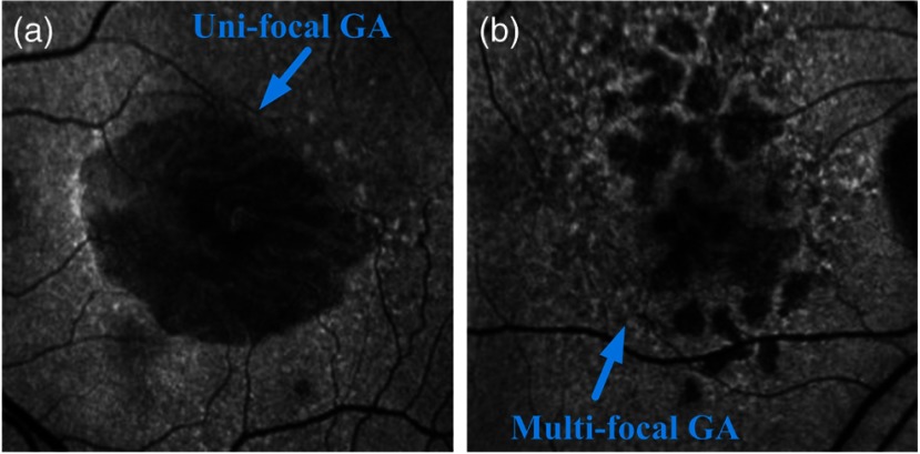
Clinically, GA is identified by the presence of depigmentation, sharply demarcated borders, and increased visibility of the underlying choroidal vessels.^1,2 Typically, the atrophic areas initially appear in the extrafoveal region in the macula,³ with eventual growth and expansion into the fovea, resulting in vision loss and, ultimately, legal blindness. Although GA accounts for one-third of the cases of late AMD and is responsible for 20% of the cases of severe visual loss due to the disorder, it currently lacks effective treatment, whereas antiangiogenic therapies have been shown to be successful in managing the other form of late AMD of choroidal neovascularization (CNV).^1,2 A number of potential agents are currently in clinical investigation to determine if they are of benefit in preventing the development and growth of these atrophic lesions. Techniques to rapidly and precisely quantify atrophic lesions would appear to be of value in advancing the understanding of the pathogenesis of GA lesions and the level of effectiveness of these putative therapeutics. Color fundus photography has been the gold standard method for documenting and measuring the size of GA lesions historically. Although GA lesions can be readily identified and demarcated in high-quality color images with good stereopsis, the borders may be more difficult to identify in monoscopic images of lower quality. Recently, fundus autofluorescence (FAF), obtained by confocal scanning laser ophthalmoscopy (cSLO) FAF imaging, has emerged as a useful imaging technique to provide a high contrast for the identification of GA lesions. FAF imaging is a noninvasive, in vivo two-dimensional imaging technique for metabolic mapping of naturally or pathologically occurring fluorophores (in lipofuscin) of the ocular fundus.⁴ FAF signals are reliable markers of lipofuscin in RPE cells. Abnormally increased lipofuscin accumulations, which produce hyperfluorescent FAF signals, occur in earlier stages of AMD. However, when atrophy ensues, RPE cells are lost and this concurrently results in the depletion of the fluorophores and a reduction in the autofluorescent signal. The FAF signal from that region becomes hypofluorescent dark. Hypofluorescence is the FAF hallmark of GA. Based on the number of atrophic areas present in the FAF images, GA could be classified into two configurations, unifocal (i.e., single) or multifocal patches. Figure 1 is an illustration of the two different GA configurations.

Fig. 1.

Illustration of the geographic atrophy (GA): (a) unifocal GA pattern and (b) multifocal GA pattern.

The reproducibility of measuring GA lesions by experienced human graders using FAF imaging has been shown to be excellent.⁵ However, the manual delineation of GA is tedious, time-consuming, and still prone to some degree of inter- and intraobserver variability by less experienced graders and clinicians in practice. Automatic detection and quantification of GA is important for determining disease progression and facilitating clinical diagnosis. Several groups have tackled this problem of automatic GA lesion detection. For example, Schmitz-Valckenberg et al.⁶ developed a semiautomated image processing approach (Heidelberg region finder) to identify GA in FAF images using a region-growing technique. Chen et al.⁷ developed a semiautomatic approach based on a geometric active contour model for segmenting GA in spectral domain optical coherence tomography (SD-OCT) images. We⁸ recently reported a level-set-based approach to segment GA lesions in SD-OCT and FAF images. The algorithm- and manually-defined GA regions in both modality images demonstrated a good agreement. However, the above approaches including ours were all semiautomatic, which decreased the efficiency of the algorithm performance, especially when multifocal GA lesions were present. More recently, Ramsey et al.⁹ reported a fuzzy c-means clustering algorithm which could detect GA lesions in a fully automated way. However, due to a well-known issue of oversegmentation with such an approach, the users needed to define the region(s) of interest (ROIs) in each image to achieve good algorithm performance. Such an approach was effectively semiautomatic due to the human interaction required for each image.

A fully automated approach without human interaction, which is able to batch process the image sets, could potentially save users’ time, especially in the case of analyzing large datasets or when multifocal GA lesions are present. Supervised classification techniques have been used for fully automated image segmentation in retinal images and have demonstrated good performance.^10–12 A key component of a supervised classification technique is identifying the proper image features. The suitability of using image texture features to classify tissues has been shown in previous studies.^10,13 GA lesions exhibit different textural features (as well as intensity and Gaussian features) from normal regions because of the differences in optical properties. Thus, the purpose of this study is to develop a novel supervised classification approach using image texture features (in addition to intensity and Gaussian features) for the fully automated segmentation of GA lesions and to compare the segmentation performance with manual delineation from an expert certified grader.

2. Methods

2.1. Overview

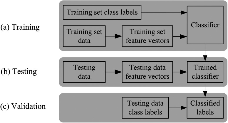
Supervised classification has been reported as an effective automated approach for the detection of AMD lesions.¹⁰ Recall that supervised classification is a machine learning task which can be divided into two phases, i.e., the learning (training) phase and the classification (testing) phase.¹⁴ The training data consist of a set of training samples. Each sample is a pair consisting of the feature vectors and a label. In the training phase, the supervised classification algorithm analyzes the labeled training data and produces classification rules. In the testing phase, the unseen new test data are classified into classes (labels) based on the generated classification rules. The classified labels are then compared with the labeled test data to validate the performance of the supervised classification. Figure 2 is an overview of the supervised classification.

Fig. 2.

Overview of supervised classification.

In this study, a supervised pixel classification algorithm using a $k$-nearest-neighbor ($k$-NN) pixel classifier¹⁵ is applied to identify GA lesions from the image features, including region-wise intensity (mean and variance) measures, gray-level co-occurrence matrix measures (angular second moment, entropy, and inverse difference moment),^16,17 and Gaussian filter banks.

2.2. Feature Extraction

The size of GA lesions varies considerably. In many cases, unifocal GA lesions could be larger and multifocal GA lesions could be smaller as shown in Fig. 1. To be able to segment both uni- and multifocal GA lesion patterns, the image feature extraction is performed on the underlying regions of the FAF gray-value image $I[x,y]$ with a sliding window of varying sized $s_x*s_y=2n*2n$, $n\in \{\mathrm{1,2},\dots 7\}\text{pixels}$. Such a convention is applied on the intensity and gray-level co-occurrence matrix measures. For the Gaussian filter banks, the filter sizes are defined by different Gaussian scales.

Specifically, the intensity level measures used in this study include the region-wise mean intensity and intensity variance, which are extracted from the original gray-value images $I[x,y]$. The sizes of the regions are defined by the sliding windows. The mean intensity value measures the image brightness and the intensity variance measures the image contrast.

A gray-level co-occurrence matrix $P[i,j]$ (Refs. 16 and 17) describes the spatial relationships that the intensity tones have to one another. It is defined by specifying an offset vector $d=(\mathrm{d}x,\mathrm{d}y)$ and counting all pairs of pixels separated by the offset $d$, which have gray values $i$ and $j$. In our case of obtaining the gray-level co-occurrence matrices from a FAF image, the gray values of the original FAF image $I[x,y]$ are first converted from 0 to 255 to the range 0 to 15, resulting in 16 gray levels from 0 to 15. We then count all the pixel pairs having the gray value $i$ in the first pixel and the gray value $j$ in the second pixel separated by the offset $d=(\mathrm{d}x,\mathrm{d}y)$. The offsets are defined by varying values $(\mathrm{d}x,\mathrm{d}y)\in \{(\mathrm{1,1}),(\mathrm{3,3}),(\mathrm{5,5})\dots ,(\mathrm{15,15})\}$; pixels when they are within the sizes of the regions. Since the converted gray values have 16 levels, the resulted gray-level co-occurrence matrices (a set of resulted $P[i,j]$ matrices satisfying the specified offsets) have the size of $16\times 16$.

The gray-level co-occurrence matrices are important because they can capture the spatial dependence of gray-level values through the resulted texture features. More specifically, in our case, three textural features, i.e., angular second moment, entropy, and inverse difference moment, are extracted from each gray-level co-occurrence matrix.^16,17

The angular second moment is a strong measure of the gray-level uniformity.

$$\text{Angular second moment}=\sum _i\sum _j{P}^2[i,j].$$ (1)

The entropy measures the randomness of gray-level distribution.

$$\text{Entropy}=\sum _i\sum _{j}P[i,j]\log P[i,j].$$ (2)

The inverse difference moment measures the local homogeneity.

$$\text{Inverse difference moment}=\sum _i\sum _j\frac{1}{1+{(i-j)}^2}P[i,j].$$ (3)

These features are important because they reflect the changes of image texture in GA regions from normal regions, which can help distinguish GA regions from the background.

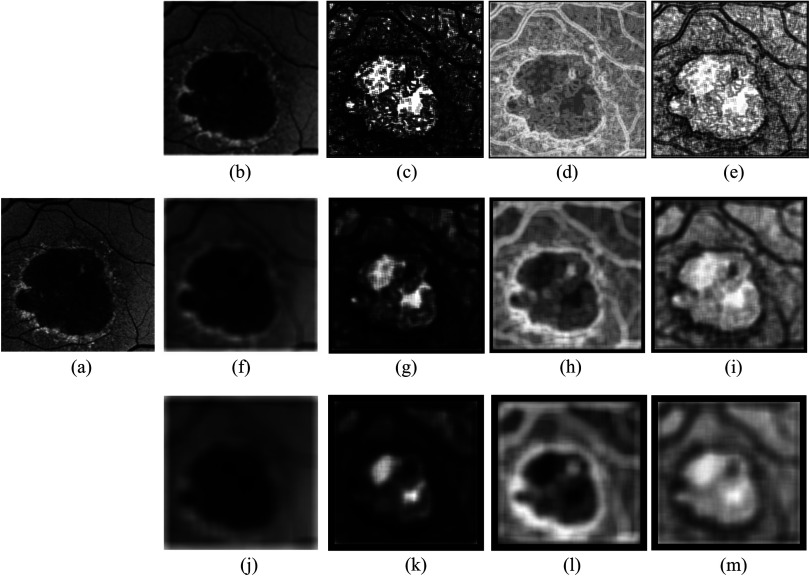
A Gaussian filter bank with eight Gaussian scales at $\sigma =8n$, $n\in \{\mathrm{1,2},\dots 8\}\text{pixels}$ is applied to blur the original gray-value image $I[x,y]$. The Gaussian filters are applied only in the $x$- and $y$-directions. The different Gaussian scales define the different filter sizes and the sliding windows are not applied to the Gaussian feature extraction. In addition to the above features, the original gray-value intensity image $I[x,y]$ is also included in the image feature space. Figure 3 is an illustration of a few randomly selected image features. After extracting the image features, each feature vector is normalized to zero mean and unit variance.

Fig. 3.

Illustration of varying size image features. (a) Original fundus autofluorescence (FAF) image. (b) to (e) Image features with a sliding window size of $s_x*s_y=2*2$ pixels with (b) mean intensity, (c) angular second moment, (d) entropy, and (e) inverse difference moment extracted from gray-level co-occurrence matrix with $(dx,dy)=(\mathrm{3,3})$. (f) to (i) Image features with a sliding window size of $s_x*s_y=6*6$ pixels with (f) mean intensity, (g) angular second moment, (h) entropy, and (i) inverse difference moment extracted from gray-level co-occurrence matrix with $(dx,dy)=(\mathrm{5,5})$ pixels. (j) to (m) Image features with a sliding window size of $s_x*s_y=12*12$ pixels with (j) mean intensity, (k) angular second moment, (l) entropy, and (m) inverse difference moment extracted from gray-level co-occurrence matrix with $(dx,dy)=(\mathrm{7,7})$ pixels.

2.3. $k$-NN Classification

The supervised pixel classification includes a training phase and a testing phase, which are performed in a set of training data and that of testing data, respectively. In this study, the entire dataset is split into two subsets with equal image numbers. The two subsets are interchanged to be used as training and testing sets, respectively. To reduce the bias of the classification, the two subsets are shuffled as described in Sec. 3 to obtain eight training sets and eight corresponding testing sets. At the training stage, the image feature vectors are obtained from each training image and combined together to obtain the feature vectors for the entire training set. Each sample/pixel in the training set is labeled as two classes of GA or non-GA as the ground truth for the training. The testing is performed on each individual image in the testing set. Similarly, each sample/pixel in the testing set is also labeled as two classes of GA or non-GA as the ground truth for the testing.

A $k$-NN classifier¹⁵ is a supervised classifier that classifies each sample/pixel on an unseen test image based on a similarity measure, e.g., distance functions with the training samples. In our case, a sample/pixel is classified as GA or non-GA by a majority vote of its $k$ ($k=31$) neighbors in the training samples being identified as GA or non-GA. To save the execution time, in this work, the searching of the NN training samples/pixels for each query sample/pixel is implemented using an approximate NN approach,¹⁸ with a tolerance of a small amount of error, i.e., the searching algorithm could return a point that may not be the NN, but is not significantly further away from the query sample/pixel than the true NN. The error bound $ϵ$ is defined such that the ratio between the distance to the found point and the distance to the true NN is less than $1+ϵ$ and the $ϵ$ is set to 0.1 in this study. Based on the obtained $k$-NN training samples/pixels, each query sample/pixel in the test image is assigned to a soft label $p_{\mathrm{GA}}$:

$$p_{\mathrm{GA}}=n/k,$$ (4)

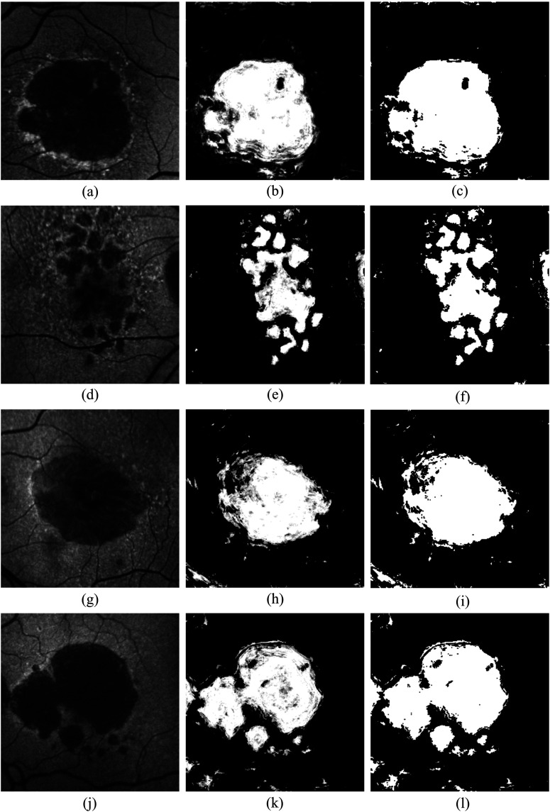
where $n$ is the number of training samples/pixels labeled as GA among the $k$-NN training samples/pixels. The soft label represents the posterior probability of that query sample/pixel belonging to the GA lesion. This results in a GA probability map, representing the likelihood that the image pixels belong to GA (middle column in Fig. 5). In the GA probability map, there are some small GA regions misclassified as background (referred as holes). As a postprocessing step, a voting binary hole-filling filter¹⁹ is applied to fill in the small holes. More specifically, centered at a pixel, in its neighborhood $R_x/2$ by $R_y/2\text{pixels}$, the hole-filling filter iteratively converts the background pixels into the foreground until no pixels are being changed or until it reaches the maximum number of iterations. The rule of the conversion is that a background pixel is converted into a foreground pixel if the number of foreground neighbors surpasses the number of background neighbors by a majority value ($[(R_x*R_y-1)/2]+\text{majority}$) in that neighborhood. In this study, by the observation of the hole sizes, the neighborhood is set to size of $7\times 7\text{pixels}$, the majority value is set to 2, and the iteration is set to 5. Some example results of the hole-filling filter are shown in the right column of Fig. 5.

Fig. 5.

Illustration of GA segmentation results. Left, middle, and right columns indicate the original FAF images, GA segmentation result, and the GA segmentation after hole-filling, respectively. The proposed algorithm can be applied to both uni- and multifocal GA detection and classification. Note the false positives from the blood vessels in the segmented images of row 3 and row 4.

3. Experimental Approach

Sixteen subjects with late-stage AMD and evidence of GA were recruited from the University of Southern California Retina Clinics. Subjects with evidence of CNV as determined by imaging and ophthalmoscopic examination were excluded as well as patients with other ocular diseases or atrophy due to disease aside from AMD. For each subject, both eyes underwent FAF imaging using a Heidelberg cSLO (Spectralis HRA+OCT, Heidelberg Engineering, Heidelberg, Germany). The image resolution used in this study is $512\times 512\text{pixels}$ and the physical dimensions as provided by the camera system are $6\mathrm{mm}\times 6\mathrm{mm}$. One eye of each subject is randomly chosen to perform the supervised pixel classification.

Manual delineation (labeling) of GA regions (as described in Sec. 2.3) for both the training and testing aim is performed on the 16 randomly selected FAF images by a certified grader of Doheny Image Reading Center. To evaluate the algorithm performance, the 16 images are first equally split into two subsets and used as training and testing sets interchangeably. We then shuffle the training and testing sets three times by selecting four images from the training set and four images from the testing set to obtain a new training set, with the remainder used as the testing set. This results in a total of eight training sets and eight corresponding testing sets to perform the eight-fold cross-validation. For each fold, the training samples are $512\times 512\times 8=\mathrm{2,097,152}$ pixels for the entire training set images and the test samples are $512\times 512=\mathrm{262,144}\text{pixels}$ for each test image. For computational efficiency, a random selection, which randomly selects 50% of the training samples (each training sample includes the multiple features corresponding to that sample) from each training set, is applied to reduce the training sample size.

The algorithm performance is evaluated against the manual delineation by mean and absolute mean GA area, mean and absolute mean GA area difference, overlap ratio (OR),⁷ Pearson’s correlation coefficient (Pearson’s $r$),²⁰ accuracy (ACC), sensitivity or true positive rate (TPR), specificity (SPC) or true negative rate, precision or positive predictive value (PPV), and false discovery rate (FDR),²¹ respectively.

OR measures the spatial overlap of GA region $A$ from the algorithm segmentation and the corresponding GA region $B$ from manual delineation.

$$\mathrm{OR}(A,B)=(A\cap B)/(A\cup B).$$ (5)

Pearson’s $r$ measures the area correlation between region $A$ and $B$ for all the $n$ test images.

$$r=\frac{{\sum }_{i=1}^n(A_i-\overline{A})(B_i-\overline{B})}{\sqrt{{\sum }_{i=1}^n{(A_i-\overline{A})}^2}\sqrt{{\sum }_{i=1}^n{(B_i-\overline{B})}^2}}.$$ (6)

ACC measures the proportion of the actual GA (positive, $P$) and actual non-GA (negative, $N$) pixels, which are correctly identified as GA (true positive, TP) and non-GA (true negative, TN).

$$\mathrm{ACC}=(\mathrm{TP}+\mathrm{TN})/(P+N).$$ (7)

TPR measures the proportion of the actual GA ($P$) pixels that are correctly identified as GA (TP) lesions. The actual GA is equal to the correctly identified GA (TP) plus the GA identified as background (FN).

$$\mathrm{TPR}=\mathrm{TP}/P=\mathrm{TP}/(\mathrm{TP}+\mathrm{FN}).$$ (8)

SPC measures the proportion of the actual non-GA ($N$) pixels that are correctly identified as non-GA (TN) lesions. The actual non-GA is equal to the correctly identified non-GA (TN) plus the non-GA identified as GA (FP).

$$\mathrm{SPC}=\mathrm{TN}/N=\mathrm{TN}/(\mathrm{FP}+\mathrm{TN}).$$ (9)

PPV measures the proportion of the correctly identified GA (TP) pixels over all the GA identified.

$$\mathrm{PPV}=\mathrm{TP}/(\mathrm{TP}+\mathrm{FP}).$$ (10)

FDR measures the proportion of the non-GA that is identified as GA (FP) over all the GA identified.

$$\mathrm{FDR}=\mathrm{FP}/(\mathrm{TP}+\mathrm{FP})=1-\mathrm{PPV}.$$ (11)

4. Results

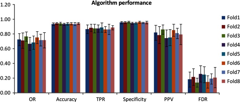
Table 1 displays the mean values of the algorithm- and manually defined GA regions for the eight-fold cross-validation in terms of the parameters of GA area, Pearson’s $r$ (area correlation), OR, ACC, TPR, SPC, PPV, and FDR. Figure 4 illustrates the results of OR, ACC, TPR, SPC, PPV, and FDR for each fold. Figure 5 is an example illustration of the GA segmentation for both the unifocal patterns and the multifocal patterns.

Table 1.

Mean area comparison of algorithm and manually defined geographic atrophy regions of the eight-fold cross-validation.

Mean area (${\mathrm{mm}}^2$) (algorithm)	Mean area (${\mathrm{mm}}^2$) (manual)	Mean correlation of area	Mean area difference (${\mathrm{mm}}^2$)a	Absolute mean area difference (${\mathrm{mm}}^2$)	Percentage of mean area differenceb	Percentage of absolute mean area differenceb
$7.24\pm 0.67$	$6.84\pm 0.98$	$0.98\pm 0.02$	$0.40\pm 0.33$	$0.94\pm 0.55$	$0.11\pm 0.08$	$0.18\pm 0.08$
Overlap ratio	Accuracy	True positive rate		Specificity	Positive predictive value	False discovery rate
$0.72\pm 0.03$	$0.94\pm 0.00$	$0.87\pm 0.01$		$0.96\pm 0.01$	$0.80\pm 0.04$	$0.20\pm 0.04$

^aPositive value implies that the mean algorithm-defined area is greater than that from the manual delineation.

^bPercentage value is defined as the corresponding mean area difference over the area of manual delineation.

Fig. 4.

Algorithm segmentation performance versus manual delineation of the eight-fold cross-validation.

5. Discussion

In this study, we present a novel supervised pixel classification approach for automated GA segmentation in FAF images. The supervised pixel classification uses the $k$-NN classifier and the image features include region-wise intensity measures, gray-level co-occurrence matrix based textural measures, and Gaussian measures. The algorithm performance is validated using eight-fold cross-validation against the manual segmentation. As shown in Table 1, the algorithm- and manually defined GA regions overall demonstrate a good agreement.

The major advantage of our supervised pixel classification approach for GA segmentation compared to previous approaches by others^6,7,9 and our previous level-set-based approach⁸ is that it is fully automated and does not require a manual selection of seed point(s) or user-defined ROIs. This is important when there is a large dataset needing to be processed or when there are multifocal GA patches, as our algorithm could batch process the whole dataset without any user interaction. Hence, one can expect it to be easier to use and faster. In addition, multiple image features, e.g., the intensity, textural, and Gaussian features as shown in this study, can be easily incorporated to the feature vectors for the classification. Moreover, the varying sized region-wise and scale-based features enable the detection of both uni- and multifocal GA lesions. This is another advantage of the supervised classification approach. Furthermore, our supervised classification detects the foreground of the darker region(s) and classifies each pixel in the test image as GA or non-GA. Abràmoff et al.¹¹ have applied supervised classification approaches for segmentation of the optic cup and rim in human eyes. Gossage et al.¹³ have used image texture features to classify normal and abnormal mouse tissues. Our detection and classification framework using textural features should be adaptable for use in the detection of other structures or diseases (not just macular degeneration), by classifying them into different categories based on differences in available image features.

Our algorithm is evaluated against the ground-truth manual segmentation performed by the certified grader. Since we do not find other fully automated GA segmentation approaches reported, we have compared our segmentation performance with the semiautomated approach reported by Chen et. al.⁷ In Chen’s paper, the primary application of their algorithm was on the segmentation of GA lesions in OCT images. The algorithm was also applied to FAF images. They reported a high level of segmentation accuracy. The OR between (1) their approach and outlines drawn in the SD-OCT scans, (2) their approach and outlines drawn in the FAF images, and (3) the commercial software (Carl Zeiss Meditec proprietary software, Cirrus version 6.0) and outlines drawn in FAF images were 72.60, 65.88, and 59.83%, respectively. As shown in Table 1, the mean OR between our approach and manual segmentation in the FAF images was 72.00%. Thus, our automated results are comparable with Chen’s semiautomated approach, though it is important to note that our image datasets are not the same.

Despite the favorable performance of the GA segmentation in this preliminary study, the validation results in Table 1 indicate that the algorithm still has room for improvement. For instance, the OR reflected the spatial overlap of the algorithm- and manual-defined GA. The mean OR of the eight-fold cross-validation is $0.72\pm 0.03$, which means there is some mismatch of the algorithm- and manual-defined GA regions. The sensitivity or TPR measures the proportion of the actual GA pixels that are correctly identified as GA lesions. The mean sensitivity (or TPR) of the eight-fold cross-validation is $0.87\pm 0.01$, indicating the algorithm misses some atrophy. There are also some false positives (non-GA is identified as GA) as indicated by the mean false discovery rate of $0.20\pm 0.04$. In addition, the mean false discovery rate and mean sensitivity indicate that the chance of non-GA being identified as GA is larger than the missed detection of GA. One possible solution to enhance the performance of both missed detection and false discovery of GA is to incorporate other image features, for instance, wavelet-transform-based image features.¹⁰ Wavelet transform has been reported to be able to help remove the speckling and other high-frequency noises. It also provides a great ability to selectively utilize the desired coarse or fine image features and, hence, is expected to improve the segmentation performance for both the unifocal and multifocal GA patterns. In addition, for the false discovery, the false positives from the retinal blood vessels (as shown in rows 3 and 4 of Fig. 5) are a major source. This issue can be resolved, however, using our previously reported vessel segmentation algorithm¹² to identify the vessel locations and exclude them from the feature vectors in the $k$-NN classification process.

In summary, in this study, a novel $k$-NN supervised pixel classification approach for the automated GA segmentation in FAF images is developed. The algorithm performance is tested using eight-fold cross-validation and demonstrates a good agreement between the algorithm- and manually defined GA regions.

Biography

Biographies of the authors are not available.

References

- 1.Klein R., et al. , “Changes in visual acuity in a population over a 15 year period: the Beaver Dam Eye Study,” Am. J. Ophthalmol. 142, 539–549 (2006). 10.1016/j.ajo.2006.06.015 [DOI] [PubMed] [Google Scholar]
- 2.Blair C. J., “Geographic atrophy of the retinal pigment epithelium: a manifestation of senile macular degeneration,” Arch. Ophthalmol. 93, 19–25 (1975). 10.1001/archopht.1975.01010020023003 [DOI] [PubMed] [Google Scholar]
- 3.Sarks J. P., Sarks S. H., Killingsworth M. C., “Evolution of geographic atrophy of the retinal pigment epithelium,” Eye 2, 552–577 (1988). 10.1038/eye.1988.106 [DOI] [PubMed] [Google Scholar]
- 4.Schmitz-Valckenberg S., et al. , “Fundus autofluorescence imaging: review and perspectives,” Retina 28, 385–409 (2008). 10.1097/IAE.0b013e318164a907 [DOI] [PubMed] [Google Scholar]
- 5.Khanifar A. A., et al. , “Comparison of color fundus photographs and fundus autofluorescence images in measuring geographic atrophy area,” Retina 32(9), 1884–1891 (2012). [DOI] [PMC free article] [PubMed] [Google Scholar]
- 6.Schmitz-Valckenberg S., et al. , “Semiautomated image processing method for identification and quantification of geographic atrophy in age-related macular degeneration,” Invest. Ophthalmol. Vis. Sci. 52(10), 7640–7646 (2011). 10.1167/iovs.11-7457 [DOI] [PubMed] [Google Scholar]
- 7.Chen Q., et al. , “Semi-automatic geographic atrophy segmentation for SD-OCT images,” Biomed. Opt. Express 4(12), 2729–2750 (2013). 10.1364/BOE.4.002729 [DOI] [PMC free article] [PubMed] [Google Scholar]
- 8.Hu Z., et al. , “Segmentation of the geographic atrophy in spectral-domain optical coherence tomography volume scans and fundus autofluorescene images,” Invest. Ophthalmol. Vis. Sci. 54(13), 8375–8383 (2013). 10.1167/iovs.13-12552 [DOI] [PubMed] [Google Scholar]
- 9.Ramsey D. J., et al. , “Automated image alignment and segmentation to follow progression of geographic atrophy in age-related macular degeneration,” Retina 34(7), 1296–1307 (2014). 10.1097/IAE.0000000000000069 [DOI] [PubMed] [Google Scholar]
- 10.Quellec G., et al. , “Three-dimensional analysis of retinal layer texture: identification of fluid-filled regions in SD-OCT of the macula,” IEEE Trans. Med. Imaging 29, 1321–1330 (2010). 10.1109/TMI.2010.2047023 [DOI] [PMC free article] [PubMed] [Google Scholar]
- 11.Abràmoff M. D., et al. , “Automated segmentation of the cup and rim from spectral domain OCT of the optic nerve head,” Invest. Ophthalmol. Vis. Sci. 50, 5778–5784 (2009). 10.1167/iovs.09-3790 [DOI] [PMC free article] [PubMed] [Google Scholar]
- 12.Hu Z., et al. , “Automated segmentation of 3-D spectral OCT retinal blood vessels by neural canal opening false positive suppression,” Lec. Notes Comput. Sci. 6363, 33–40 (2010). 10.1007/978-3-642-15711-0 [DOI] [PubMed] [Google Scholar]
- 13.Gossage K. W., et al. , “Texture analysis of optical coherence tomography images: feasibility for tissue classification,” J. Biomed. Opt. 8(3), 570–575 (2003). 10.1117/1.1577575 [DOI] [PubMed] [Google Scholar]
- 14.Mohri M., Rostamizadeh A., Talwalkar A., Foundations of Machine Learning, The MIT Press, Cambridge, Massachusetts: (2012). [Google Scholar]
- 15.Duda R., Hart P., Stork D., Pattern Classification, 2nd ed., John Wiley and Sons, New York: (2001). [Google Scholar]
- 16.Jain R., Kasturi R., Schunck B. G., Machine Vision, McGraw-Hill, Inc., New York: (1995). [Google Scholar]
- 17.Sharma N., et al. , “Segmentation and classification of medical images using texture-primitive features: application of BAM-type artificial neural network,” J. Med. Phys. 33(3), 119–126 (2008). 10.4103/0971-6203.42763 [DOI] [PMC free article] [PubMed] [Google Scholar]
- 18.Arya S., et al. , “An optimal algorithm for approximate nearest neighbor searching in fixed dimensions,” J. ACM 45(6), 891–923 (1998). 10.1145/293347.293348 [DOI] [Google Scholar]
- 19.Ibàñez L., et al. , The ITK Software Guide, 2nd ed., Kitware, Inc; (2005). [Google Scholar]
- 20.Hollander M., Wolfe D. A., Nonparametric Statistical Methods, pp. 185–194, John Wiley & Sons, New York: (2013). [Google Scholar]
- 21.Lalkhen A. G., McCluskey A., “Clinical tests: sensitivity and specificity,” Contin. Educ. Anaesth. Crit. Care Pain 8(6), 221–223 (2008). 10.1093/bjaceaccp/mkn041 [DOI] [Google Scholar]