Abstract.
An artifact found in magnetic resonance images (MRI) called partial volume averaging (PVA) has received much attention since accurate segmentation of cerebral anatomy and pathology is impeded by this artifact. Traditional neurological segmentation techniques rely on Gaussian mixture models to handle noise and PVA, or high-dimensional feature sets that exploit redundancy in multispectral datasets. Unfortunately, model-based techniques may not be optimal for images with non-Gaussian noise distributions and/or pathology, and multispectral techniques model probabilities instead of the partial volume (PV) fraction. For robust segmentation, a PV fraction estimation approach is developed for cerebral MRI that does not depend on predetermined intensity distribution models or multispectral scans. Instead, the PV fraction is estimated directly from each image using an adaptively defined global edge map constructed by exploiting a relationship between edge content and PVA. The final PVA map is used to segment anatomy and pathology with subvoxel accuracy. Validation on simulated and real, pathology-free T1 MRI (Gaussian noise), as well as pathological fluid attenuation inversion recovery MRI (non-Gaussian noise), demonstrate that the PV fraction is accurately estimated and the resultant segmentation is robust. Comparison to model-based methods further highlight the benefits of the current approach.
Keywords: neuroimaging, image analysis, tissue segmentation, magnetic resonance imaging, partial volume averaging
1. Introduction
Analyzing magnetic resonance images (MRI) of the brain often requires an accurate tissue segmentation of the gray matter (GM), white matter (WM), cerebrospinal fluid (CSF), and pathology. Manual segmentation of these tissues by an expert is time-consuming, labor-intensive, subjective, and error-prone since many structures must be manually outlined for several images per patient. To combat these challenges, automated techniques may be used since they offer efficient, objective, repeatable, and quantitative segmentations.
A common challenge of automatic MR brain segmentation is the partial volume averaging (PVA) artifact, which concerns the way a volume element is imaged when there is more than one tissue present within the extent of the voxel. PVA can lead to 30% to 60% error in the volume measurement of complex brain structures1–3 and, therefore, must be taken into account to ensure that segmentations are accurate and volume measurements are precise. The most commonly used PVA model assumes each intensity value in the image is the weighted sum of random variables, each of which represents a pure tissue class.3,4 The weighting factor is referred to as the partial volume (PV) fraction, which describes the percentage of each tissue present in the voxel.
The process of estimating the PV fraction for every pixel is usually performed in two stages.3,5 First, a PV classification step finds class labels for the pure tissue and mixture (PVA) classes, which is used to estimate distributional parameters for each class. Following this, the PV fraction is estimated using the parameters found during the PV classification step.
The most popular method of PV classification is based on Bayesian frameworks and an image histogram that is approximated by mixture models constructed with a priori class distributions.2–4,6–8 Usually, Gaussian intensity models with equal variances are used to represent the intensity distributions of the pure tissue classes, and the PVA voxels are modeled by a separate Gaussian,9 as a combination of the neighboring tissue classes’ Gaussians6 or as a uniform distribution.2 These works are foundational and provide critical understanding of PVA.
After PV classification, the PV fraction is estimated using the maximum-likelihood principle (usually assuming equal tissue type variances).3–5 As discussed in these papers, the accuracy of PV fraction is strongly affected by noise, as well as the accuracy of the parameter estimation phase. To combat noise, some works have employed Markov random fields as well as noise filtering methods and have achieved promising results.3–5 However, even a small amount of error in the parameter estimation phase causes huge amounts of error in the estimate of the PV fraction.3
The accuracy of the parameters is directly related to the probability distribution function (PDF) that is chosen to represent the tissue classes. Therefore, models would need to be accurately chosen for pure tissues, PVA classes, as well as a pathology class (if present). Most often Gaussian models are selected since it eases parameter estimation and has been shown to be related to images acquired with single-coil acquisition systems with high signal-to-noise ratios.10 However, there are challenges with these approaches: newer (multicoil) acquisition systems generate non-Gaussian noise with distributions that are often unknown or mathematically intractable;10 there is no explicit mathematical model for PVA even in the presence of Gaussian noise,5 and pathology generally does not follow any known mathematical distribution. In these scenarios, previous works are suboptimal since Gaussian distributions do not accurately represent tissues, which leads to inaccurate parameter and PV fraction estimation. Other authors have noted the selection of a Gaussian model as controversial.5
Preselecting a model or distribution that can handle tissue classification for images with non-Gaussian noise and pathology classes in one is very difficult. Therefore, in this work, we focus on avoiding the pre-selection of a distribution a priori by developing a generalized methodology that is based on the inherent properties of the image, instead of noise statistics and models of pathology. It can perform brain tissue segmentation for all types of scenarios within one framework, and also avoids expectation maximization (EM) for parameter estimation, which is computationally complex and local.6
There are nonparametric classification techniques in the literature that attempt to overcome model-selection issues by processing coregistered, multicomponent datasets [i.e., T1, T2, proton density (PD)].11–13 Redundancy removes dependency on distributional parameters, but the classification result is not a PV fraction. Rather the result is a probability value that describes the likelihood or degree of membership to a particular class.5 Increased image acquisition cost (several modalities per patient), computational complexity, memory requirements, as well as registration errors further reduce the appeal of such approaches.
The current work is a computationally efficient, model-independent approach that operates on a single modality to estimate the PV fraction directly from the image by exploiting a mathematical relationship between edge content and PVA. The proposed work is generalized in that it does not make any assumption regarding the underlying tissue classes or noise distribution. As a result, it can operate on normal and abnormal images (with/without pathology) as well as those acquired by both single coil and multicoil technologies (contaminated by Gaussian or non-Gaussian noise). To the best of our knowledge, the proposed work is one of the only techniques that can efficiently handle all these scenarios within a single framework. The method is validated and compared to model-based approaches for several databases: simulated and real T1 MRI with no pathology and Gaussian noise, as well as fluid attenuation inversion recovery (FLAIR) MRI with white matter lesions (WML) and non-Gaussian noise.
The paper is structured as follows. Section 2 describes the motivation and mathematical foundations of the current approach, Sec. 3 describes the image processing methods used to implement the approach, and Sec. 4 contains the results.
2. Motivation and General Framework
Consider a neurological MR image denoted by , where each voxel has an intensity at spatial location . In pure tissue regions (single tissue type within the voxel), the intensity is drawn from a probability distribution, i.e., , where and is the tissue type. In PVA voxels, there are usually two tissues present within the extent of the voxel. (In neurological MRI, PVA is considered to have two pure tissues mixing per PVA voxel since the number of voxels with more than two tissue types is negligible.2–4) The intensity of these mixture pixels is determined by the PV fraction (percentage of tissue versus tissue ),2,6 as in:
| (1) |
where , is the intensity value of tissue drawn from , and is the intensity value selected from for tissue . The mixel class occurs over specific intensity ranges that are bounded, i.e., , whereas the two pure classes correspond to approximately unique intensity values , . A direct consequence is that PVA voxels occur in edgy regions of the image, whereas pure tissue classes occur in the flat regions. Since PVA occurs in tissue boundaries, this work seeks a relation between the edge content and PV fraction .
To ensure PV fraction estimation is accurate, noise filtering and bias field reduction should be employed first.5 Assuming noise filtering and bias field reduction have been employed, the following ideal (noise-free) signal model is realized:
| (2) |
where , are constant gray-level values uniquely depicting each tissue, and . Using the ideal signal model, we formulate a relationship between the PV fraction and the edge content in the image by taking the gradient, as in
| (3) |
where is the change in the tissue fraction between tissue and tissue . Solving for the change in tissue fraction results in a unique PVA quantifier
| (4) |
which is a normalized and class specific representation of edge information in PVA regions. It is normalized because the largest possible value of is (step-edge or maximum intensity change in one pixel step) and the minimum is 0 in a constant region, resulting in . It is class-specific because the value is dependent on the edge information of the underlying class representation of edge information in PVA regions. This mathematical relationship directly relates the PV fraction to the edge content in the image. This is a relationship that we believe will be foundational in paving the way for many new works. The remainder of this paper will demonstrate how to exploit this relationship to estimate the PV fraction.
Considering the derivative in Eq. (4), the PV fraction may be found by integration of
| (5) |
where , , are the spatial coordinates that delineate the PVA region from the surrounding pure tissues (tissue and tissue ), is the constant of integration, and is a dummy variable used for integration. There are three main challenges with estimating the PV fraction in such a manner:
-
1.
Integration bounds: Prior knowledge of the spatial coordinates of the PVA region (, ) is needed to integrate in the spatial domain.
-
2.
Classification: The particular tissue type (i.e., ) must be identified first in order to segment tissue structures.
-
3.
Noise and tissue intensity variation: Localized edge strength measures [, ] are afflicted by noise.
The proposed work manages these three challenges in an efficient manner. Integration bounds and classification challenges are handled since classification is performed directly in the global (intensity) domain using thresholds that dynamically change depending on the image’s edge content, instead of performing it in the spatial domain. Therefore, neither is there a need to define integration bounds nor is classification a priori required with this approach. Since intensity is related to the tissue classes, estimation of the PV fraction in the global domain results in accurate tissue segmentations. Noise and tissue intensity variation is minimized by robust noise preprocessing (filtering) as discussed in Ref. 5 in addition to the fact that estimates are derived using the entire three-dimensional (3-D) volume at once.
To transform to the global domain, edge and intensity information are coupled through the conditional PDF of for a particular intensity by
| (6) |
where , , is the realization of , and is the maximum gray level in the volume. This PDF quantifies the distribution of the edge information for a specific gray level for the entire 3-D volume. In flat regions (pure tissues), there is clustering in the PDF for low edge values at the corresponding intensities. Across anatomical boundaries (PVA), high edge values dominate the PDF for the respective intensity ranges.
Using this PDF, a global estimate of the change in the tissue fraction, , is found with the conditional expectation operator. It offers the best prediction [in the mean square error (MSE) sense] of the edge content in the image, given the intensity is , as in
| (7) |
The change in the tissue fraction, , discriminates between PVA and pure tissue classes based on their respective edge content and intensity values. Intensity ranges with large edge values [maximally edgy, maxima of ] correspond to PVA regions, while intensity ranges with small edge content are linked to pure tissue classes [minimally edgy, or minima of ]. Contiguous, large amplitude regions of that are bounded by two minima constitute a PVA pulse, which describes the change in PV fraction between neighboring pure tissues, i.e., . For three tissue classes (i.e., CSF, WM, GM), there are two PVA pulses that represent the two mixture classes (CSF-WM, WM-GM) and three minima in corresponding to the pure tissue classes , . Let the minima of be denoted by , , and the maxima of the PVA pulse be denoted by , .
To compute from , voxels that are maximally edgy, i.e., PVA, are retained. Since noise generates artificial edginess, the minima of are nonzero for pure tissue regions. To find which voxels belong to the PVA class, an adaptive threshold is applied to the left and right side of each PVA pulse that retains voxels that are most probable to contain mixture components
| (8) |
| (9) |
where and are the minimum values of for pure tissue and , respectively, and is the maximum value of for the PVA pulse that describes the mixture of tissue with tissue .
To find the class-specific change in PV fraction, the adaptive thresholds are applied
| (10) |
| (11) |
where , , and are the gray levels that correspond to landmarks (optima) in (, , and ). The remaining nonzero values define , over the gray levels in the range of , which are the regions that contain large-valued edge information.
To decode the PV fraction, , each refined PVA pulse is integrated over the corresponding intensity values
| (12) |
where the denominator is a normalizing constant, such that . This PV fraction describes the proportion of each tissue found in voxels with intensity . Converting the localized edge metric into the global domain eases computation of the PV fraction.
As dictates which gray levels belong to mixture classes, it can be easily modified to get class memberships for each tissue class. Class memberships are nonzero over the gray-level values that belong to each of the classes, and the value of the membership function dictates the amount of tissue present in the voxel ( for pure tissues and for PVA voxels). The class membership for tissue is found by
| (13) |
and the class membership of tissue is computed similarly
| (14) |
These profiles describe the fractional membership of gray levels to each tissue class.
3. Image Processing Methods
The following section will describe the image processing algorithms that are used to implement the PV fraction estimation and tissue segmentation approach. The various stages are depicted in Fig. 1.
Fig. 1.

Image-based features required for partial volume averaging (PVA) quantification and brain tissue segmentation.
3.1. Estimation of
A fuzzy technique based on the cumulative distribution function (CDF) of the gradient14,15 is employed to find . First, the magnitude of the gradient, , is estimated by the Sobel operator followed by computation of the PDF of the gradient . The CDF of the gradient magnitude is found by
| (15) |
where . This nonlinear edge measure quantifies the certainty of edge presence for gradient . As shown in Refs. 14 and 16, assigns high and like values to significant edges, despite them occurring over a wide range of and with few occurrences. Therefore, it groups significant edges (edgy regions), while suppressing the irrelevant ones (flat regions). It is normalized , and to arrive at , is mapped back to the spatial domain: .
3.2. Estimation of
The conditional PDF is used to transform the localized edge metric to a global one. A kernel density estimator (KDE) is used since it creates a smoother visual construction of the frequency distribution17 compared to the empirical distribution. Given a sample of fuzzy edge values , for a specific intensity , the KDE is formed by the summation of a series of kernels for all sample data
| (16) |
where is a Gaussian kernel function and is the standard deviation of the Gaussian. Since this technique is applied in 3-D, is the total number of voxels with intensity from the 3-D volume.
To discriminate between pure tissue voxels and PVA voxels, two bin locations at and are substituted into Eq. (16), resulting in a conditional PDF that describes edge presence for each gray level for the nonedge class (pure) and edge class (PVA), respectively. The PDF for the nonedgy regions (pure tissue class) is described by
| (17) |
where the last line is valid for symmetric kernels since and . The probability that a voxel lies in a PVA region (significant edge) is found by
| (18) |
The two probability functions describe the likelihood that intensity belongs to a PVA (edge) or pure tissue (flat) class. Since they are PDFs, it is required that . [Note that KDEs estimated by numerical programs, such as MATLAB®, return histogram values, not probability values. Therefore, and are normalized to ensure ]. Since there are two classes, the number of bins are two and the size of the bins are proportional to the width of the kernel.
The support of the Gaussian kernel is roughly , where is the standard deviation of the distribution. To perform the classification, the minimum length of the support of the Gaussian should be 0.5, to ensure that there are no invalid probabilities [i.e., ]. Moreover, the maximum support of the Gaussian should also be , so the characteristic functions are not defined outside the valid range for symmetric classifiers. As a result, the scale parameter can be found by
| (19) |
which simplifies to . The smallest possible kernel in this range is taken for better discrimination between classes.
3.3. Estimating
Using the probability estimates found by Eqs. (17) and (18), the global estimate for the change in tissue fraction, , is found by the conditional expectation operator.
| (20) |
where the last line shows that the PV fraction is related to the probability that a voxel is located on an edge. Mapping back to the spatial domain [] highlights PVA voxels with large values.
3.4. Estimating Threshold
To estimate the thresholds for each PVA pulse, the optima of need to be computed to determine the ranges of the PVA pulses. An optima-finding algorithm is used to estimate , , , and . Initially, the gray-level histogram of the volumetric dataset is computed, and a peak-finding algorithm is invoked to locate the maxima of the histogram. The derivative of the histogram is taken, and the points where the derivative changes sign are used to locate candidates for and [the maxima or peaks of the histogram correspond roughly to the minima of ]. Using the initial estimates of and found in this phase, the maxima, and , are found by searching between two adjacent minima. For error checking, the minimum between two adjacent maxima are found again to ensure the correct minima were found by the peak-finding algorithm. For three pure tissues, two PVA peaks are automatically detected, along with the gray-level ranges that pure and PVA voxels span.
3.5. PV Fraction Estimation and Tissue Segmentation
The thresholds are used to solve for , and the PV fraction is decoded with Eq. (12). An example is shown in Fig. 2, as applied to the simulated image of Fig. 2(a) (three pure tissue classes and two PVA classes). The estimated PV fraction (spatial domain representation) is shown in Fig. 2(b), where the brightest voxels signify the first tissue is dominating the PVA voxel . The averaged one-dimensional scanline of the estimated PV fraction, , and the ground truth partial volume fraction, , are shown in Fig. 2(c). The estimated and true values are very similar, demonstrating the accuracy and precision of the approach. The left-most peak is the tissue fraction for the mixels, or , and the rightmost peak shows the tissue fraction for the PVA region, or .
Fig. 2.
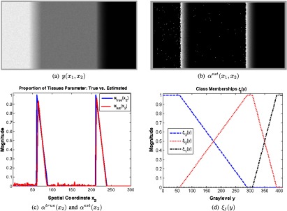
PVA fraction estimation. Top: simulated image with three pure tissues (a) and estimated partial volume fraction in two dimension (b). Bottom: Averaged (along columns) one-dimensional scanline of (b) versus the ground truth (c) and corresponding class memberships (d).
The corresponding class membership functions are shown in Fig. 2(d). Each curve automatically describes the membership of each gray level to every tissue class. The class membership functions mapped back to the spatial domain are shown in Fig. 3. The pure tissue classes are denoted by “hot” red values, and PVA voxels receive fractional values in boundaries that separate two pure tissue classes.
Fig. 3.

Spatial domain representation of class membership functions , .
4. Experiments
This section details the experimental results of the proposed work employed on a series of simulated and real neurological MRI.
4.1. Preprocessing
To ensure the approach is robust, if bias field correction is required, it may be completed by any number of methods.18 Fortunately, the experimental images already had bias field correction performed (see BrainWeb, ISBR V2.0), or have it built into the scanner (see FLAIR). To reduce the impact of noise, we employ a bilateral filter because it performs edge preserving smoothing. For the bilateral filter, two parameters must be supplied, and , which are the standard deviations of the spatial and range Gaussians. We used ( window, to retain smallest details) and to capture even faint edges, where is the maximum intensity.
4.2. Image Databases
The image databases that are used for experimentation were selected for two reasons: (1) every database has ground truth tissue masks and, thus, segmentation and PVA classification performance can be quantitatively judged and (2) the datasets represent many different different imaging scenarios, such as real/simulated images, T1/FLAIR modalities, normal/pathology (WML), Gaussian/non-Gaussian noise types. The specifications and descriptions of each of the database are listed in Table 1 and briefly discussed below.
Table 1.
Experimental databases.
| BrainWeb | ISBR V2.0 | FLAIR | |
|---|---|---|---|
| Type | Simulated T1 | Real T1 | Real FLAIR |
| Pathology | None | None | White matter lesion |
| Noise | Gaussian | Gaussian | Non-Gaussian |
| Pixel dim | |||
| Slice dim | 1 mm, 3 mm, 5 mm, 7 mm | 1.5 mm | 5 mm |
| Noise level | 1%, 3%, 5%, 7% | Unknown | Unknown |
| # of volumes | One per artifact combo | 18 patients | 25 patients |
| Ground truth | Discrete, fuzzy (partial volume averaging) | Discrete | Discrete |
| Bias field correction | Retrospective | Retrospective | Nonretrospective |
The first set of images are from McGill’s simulated BrainWeb database.19,20 These simulated images have been pivotal in validating many algorithms, especially since both the discrete tissue masks and PV fraction ground truth are supplied. BrainWeb contains simulations for various noise levels and slice thicknesses, so the performance of algorithms as a function of distortions can be tested. The noise is (approximately) normally distributed and there is no pathology present.
To test the methods on real data, the Internet Brain Segmentation Repository (IBSR) (http://neuro-www.mgh.harvard.edu/cma/ibsr), Version 2 (IBSR V2) is used (ISBR V2 is more reliable than ISBR V1 since the imaging parameters in ISBR V2 are uniform throughout, permitting fair comparison). ISBR V2 contains 18 volumetric T1 MRI (128 slices/patient), which were positionally normalized into the Talairach orientation (rotation only) and processed by bias field correction routines. Ground truth masks were generated by manual segmentations. The noise approximately follows a Gaussian distribution and there is no pathology.
An additional FLAIR MRI database is used since they possess atypical qualities: non-Gaussian noise and pathology. The database contains volumetric scans acquired with a multichannel MRI system from 25 patients with WML (this research project received Institutional ethics approval in January 2008). Volume measurements of these lesions are important in assessing a patient’s risk factor for stroke,21 and therefore, precise segmentation is critical. For validation purposes, the lesions were manually segmented by an experienced radiologist.
4.3. Performance Metrics
To analyze the PVA quantification performance, BrainWeb’s fuzzy membership maps () are compared to the estimated class memberships () through the MSE. This metric takes into consideration the fractional nature of the tissue maps. The MSE is computed by
| (21) |
where is the number of pixels in class .
For databases that have only binary (discrete) ground truths, the dice similarity coefficient (DSC)22,23 is utilized to measure similarity between binary sample sets. Let and be the binary masks of the segmentation and ground truth, respectively. The DSC is defined as
| (22) |
where denotes number of items in.
4.4. BrainWeb Database
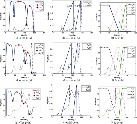
The BrainWeb database is used to quantify the performance of both PVA estimation and tissue segmentation. To estimate the conditional probability model , 3-D intensity and edge values were utilized to compute Eq. (16). This PDF is then used to find the global edge map , which is thresholded and integrated to solve for the tissue fraction for each PVA class. The corresponding functions for several simulated volumes are shown in Fig. 4. The local minima of are describing minimally edgy (flat) regions and they line up with peaks (pure voxels) in the gray-level PDF . The edgy regions (maxima) of occur in gray-level ranges that span between two pure tissues as dictated . Two separate PVA regions are detected: (left) and (right), where tissue 1 is CSF, tissue 2 is GM, and tissue 3 is WM.
Fig. 4.
Global edge (PVA) map, tissue fraction, and class memberships estimated for BrainWeb volumes. Top: 1 mm slice thickness, 1% noise level. Middle: 3 mm slice thickness, 5% noise level. Bottom: 7 mm slice thickness, 7% noise level.
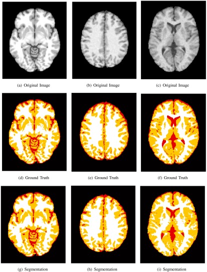
The class memberships , highlight the amount of each tissue for every intensity value. The corresponding spatial domain representations are shown in Fig. 5. A heatmap is used to display the fractional values of the masks, where a maximum value (1) receives a “hot” red color and a minimum value (0) is color coded with a “cool” blue color. The ground truth and estimated class memberships are similar in appearance, in terms of detection accuracy (location) and precision (value). Thesholding the class memberships at 0.5 results in a discrete tissue segmentation, and the results for several simulations are shown in Fig. 6. The estimated segmentation closely resembles the ground truth for several slice thicknesses and noise levels. To quantitatively validate the performance of the PVA estimation framework, the estimated and true spatial masks are compared to one another using the MSE. The average MSE for each tissue class is shown in Fig. 7.
Fig. 5.
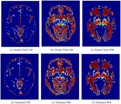
Fuzzy class membership masks for ground truth and estimated , , for 1 mm slice thickness and 1% noise.
Fig. 6.
Three BrainWeb images (top row), corresponding ground truth (middle row), and tissue segmentation (bottom row). White represents the white matter class, yellow the gray matter (GM) class, and red the cerebrospinal fluid class. Left column: 1 mm slice thickness, 1% noise level. Middle column: 3 mm slice thickness, 5% noise level. Right column: 7 mm slice thickness, 7% noise level.
Fig. 7.
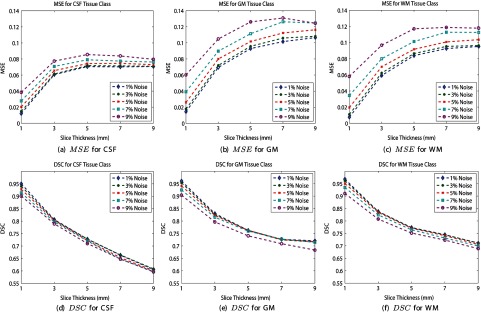
Partial volume fraction estimation and brain tissue segmentation performance for BrainWeb database. Top: mean square error. Bottom: dice similarity coefficient (DSC).
Over all slice thicknesses and noise levels, the performance is high, with over all simulation parameters and tissue types. The best performance occurs for the lowest levels of artifacts (1% noise, 1 mm slice thickness) and the lowest performance occurs for the most severe imaging artifacts (9% noise and 9 mm slice thickness).
To evaluate the tissue segmentation (detection) accuracy, the true and estimated binary tissue classification masks are compared using the DSC. The DSC for each tissue class is shown in Figs. 7(d) to 7(f). High DSC values are achieved over all slice thicknesses and noise levels for each tissue type. Interestingly, each tissue type is performing comparably (DSC trends are similar). The DSC is highest for minimal degradation and artifact levels and lowest for the most severe imaging artifacts.
An important consideration of the proposed work is the ability of the gradient to localize edge information and the dependency on the Sobel framework in different types of gradient conditions, including almost nonexistent gradient regions (“faint” edges), lesions, and/or multiscale edges.
First, the effect of the gradient on the accuracy of the PV fraction is examined in faint-edged regions (where the gradient is almost nonexistent). Mainly, such edges are created when the contrast is so low between adjacent classes and/or the noise is so high that it is difficult to differentiate between classes as seen by the gradient operator.
In images with high noise and/or low contrast, an initial denoising and/or contrast enhancement phase can be applied to enhance the results of the edge detector. There are various advanced edge-preserving smoothing filters and contrast enhancement functions that can be used, and some examples are described in this work to improve the localization capabilities of the edge detector. Additionally, as the method is a generalized framework, other edge metrics besides the Sobel operator can be applied, such as the phase congruency measure, which are less dependent on the contrast between classes. We look forward to applying these edge metrics in future work.
To analyze the performance of the Sobel operator in low-contrast/high-noise situations, the class membership maps in the GM sulci are examined further (the GM sulci are composed of a low-contrast edge between GM and WM). The class membership values are linearly related to the PV fraction and will provide good visual representation of the gradient in low-contrast regions under different noise scenarios. The resultant class membership maps for a zoomed-in region of the sulci are shown as a function of noise in Fig. 8.
Fig. 8.
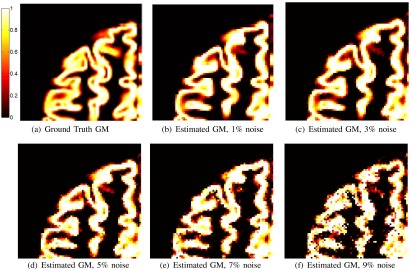
(a) Ground truth fuzzy membership mask for GM. (b) to (e) Estimated fuzzy membership mask for 1, 3, 5, 7, and 9% noise, respectively (3 mm slice thickness was used).
Visual results of the sulci demonstrate that the class membership values correlate well to the ground truth mask in low-contrast GM regions. In many of the deep sulci, the edges and GM membership were detected well. Additionally, the MSE and DSC of Figs. 7(b) and 7(e) indicate that the gradient is successful in quantifying the PV fraction over many noise levels for the GM class (which includes low-contrast regions such as sulci).
As noise is increased, the contrast-to-noise level is reduced and there is reduced performance of the algorithm. This is expected since it is a well-known fact that noise and low contrast reduces the gradient’s ability to localize edge information. Despite this, even at the highest noise levels (9% noise), the tissue segmentation produced low MSE and high DSC results [Figs. 7(b) and 7(e), and ]. Although there is noise in the estimation, there is still a high degree of similarity between the true and estimated GM masks.
We predict that the algorithm would begin to fail beyond a 9% noise level. As can be seen in Fig. 4, the difference between the maxima and minima of for the WM and GM class (in terms of amplitude) decreases for higher noise situations. Eventually, the edge will not localize and it will not be possible to detect the maxima and minima of . Fortunately, these high-noise situations are not commonly encountered in real MRI (see the results on real images in the following sections). The localization capabilities of the gradient are not affected by the presence of lesions either, which is shown later by the experimental results on the FLAIR MRI database results—that is a big advantage of this methodology.
We can now address the second concern regarding the fact that edges exist at different scales. The size of the PVA band (contiguous PVA pixels dividing two classes) is dependent on the degradation level of the PV artifact (larger slices result in more noticeable PVA). Also, different-sized objects, such as pathology, are common place. The edge information in these two cases is size dependent and, therefore, edges exist at multiple scales.
The fact that edges occur at multiple scales is a major consideration for future works. We are considering the design of a multiscale approach, which models edge information at multiple scales to estimate the PVA fraction. Inherent in this approach will be a built-in multiscale denoising scheme, which eliminates the need for preprocessing and allows us to elegantly handle the multiscale mathematics. However, this single-scale approach is foundational and paves the way for many more advanced applications, such as a multiscale one. Furthermore, results show that the localization capabilities at a single scale still produces high results, even for the 9-mm (thickest) slices [ and for the GM class as per Figs. 7(b) and 7(e)].
The effect of filtering and enhancement on performance is also an important consideration. These preprocessing stages are part of the image processing pipeline and are selected to maintain edge integrity (bilateral filtering is an edge-preserving smoothing filter). We want to estimate the true or ideal edge profiles, and this is handled through denoising in our approach. Adaptive parameters were used for the bilateral filter (function of the dynamic range of the images intensity). Therefore, this filter can be dynamically applied to a variety of images with good results.
As shown by the experimental results (see DSC and MSE of Fig. 7), the performance is excellent, indicating that despite preprocessing, the edges are maintained sufficiently and the PV fraction is estimated with high fidelity. As discussed above, we will be looking at a multiscale approach next, which includes a multiscale filtering stage. Therefore, the next version will not require any parameters to be defined, and the need for separate preprocessing is removed. However, the proposed method lays the ground work for those future approaches.
The difference between the proposed works and prior art is that there is no need to assume a Gaussian model—if the variance of the distribution (any type of distribution) is varied, the approach can handle it. This is important in modern MR systems that generate images that do not have Gaussian noise, as well as images with pathology (see results for FLAIR database).
As long as the contrast-to-noise ratio is high enough and the gradient localizes the edge information, class variability is automatically and adaptively handled without having to change anything in the method. The intensities with the highest or lowest probabilities in are automatically chosen as the maxima and minima using a peak-finding algorithm, which has several error-checking reassurances in place that double check the results. Since the most probabilistic values for the minima and maxima of have been selected, the thresholds that are defined using these values are also selected in a probabilistically sound way.
There could be some variability caused by noise that could impact the estimation of the intensity values that separate adjacent tissue classes [ or in Eq. (4)], which in turn are used to compute the threshold. Suboptimal choices for these intensity values change the intensity ranges of the pure and PVA classes and also the corresponding thresholds. The effect is usually negligible since the range between tissue classes is sufficiently large enough to reduce the impact of any small error.
If you consider Fig. 4, this point is highlighted. The figure shows the estimated class membership functions for several different noise situations (which are found by the intensity values , as well as the thresholds). As can be seen, the class memberships are very similar to one another for all of the noise scenarios and for each class. There are some minor differences contributed to noise, but that is expected as it would effect other methods, as well. However, these minor changes do not translate into gross errors, which is supported by the low MSE and high DSC results for all noise levels and slice thicknesses (Fig. 7).
In the future, error bounds or confidence intervals for PV fraction estimates will be added for uncertainty handling. The applicability of the conditional variance of is currently being considered for this.
As a final proof-point of the robustness of the proposed method, the results are compared to the results of model-based algorithms. The first comparison is with the six model-based approaches discussed in Ref. 6. The six methods, labeled A to F, encompass a variety of model-based approaches that use Gaussian mixture models, as well as spatial and anatomical priors. This paper presents a deep study of the performance of tissue modelization and classification techniques. The DSC results for these six methods as well as the proposed method, applied to T1-weighted BrainWeb images with 7% noise and 1 mm slice thickness, are reproduced in Table 2. The proposed approach outperforms methods A to F consistently and by modest amounts.
Table 2.
Dice similarity coefficient results for model-based methods (A to F),6 proposed method, and a recently developed model-based technique.24 T1-weighted BrainWeb volume, 7% noise, 1 mm slice thickness.
| A | B | C | D | E | F | Real-coded genetic algorithm | Proposed | |
|---|---|---|---|---|---|---|---|---|
| Cerebrospinal fluid | 0.83 | 0.88 | 0.81 | 0.88 | 0.77 | 0.75 | 0.92 | 0.91 |
| Gray matter | 0.71 | 0.79 | 0.70 | 0.79 | 0.70 | 0.74 | 0.89 | 0.93 |
| White matter | 0.78 | 0.88 | 0.77 | 0.89 | 0.78 | 0.89 | 0.88 | 0.94 |
Another experiment was conducted, which compares the tissue segmentation performance of the proposed work to a recently developed, open-source implementation of a model-based segmentation technique.24 This method performs tissue segmentation with finite mixture models using a real-coded genetic algorithm (RCGA) to solve the optimization problem globally. The results of the RCGA approach are listed in Table 2 as well.
The RCGA-based approach performs better than the previously developed model-based techniques (A to F) (likely as a result of the optimization improvements), but the current approach outperforms them all.
4.5. ISBR V2.0 Database
The ISBR V2.0 database is utilized to examine the performance of the technique on real images. These images contain normal anatomy (no pathology) and are contaminated by Gaussian noise. In addition to bilateral filtering preprocessing, local histogram equalization is applied to improve the signal-to-noise ratio and contrast between classes since they are low in this database.
To see the effect of histogram equalization, refer to Fig. 9. The estimated for the original image has a single defined PVA pulse and a second one of low amplitude, which is hardly distinguishable from the first one. If the contrast is too low, the gradient has limited ability to localize edge information. Using contrast enhancement, the PVA pulses are clearly defined and optima detection is successful as shown in Fig. 9(d).
Fig. 9.
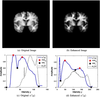
Effect of contrast enhancement on estimation of .
The estimated WM and GM class memberships for three images are shown in Fig. 10, alongside the original brain image and ground truth mask. Visually, the proposed method is robust on real images.
Fig. 10.

Brain tissue segmentation on IBSR V2.0. Top row: patient 1, middle row: patient 3, bottom row: patient 8.
For each of the 18 patients, the binary segmentation masks for the GM and WM classes were compared to the ground truth manual segmentations using the as shown in Fig. 11(a). Averaging over the entire database, the average DSC for the WM and GM tissues are 0.90 and 0.88, respectively, indicating excellent agreement.
Fig. 11.
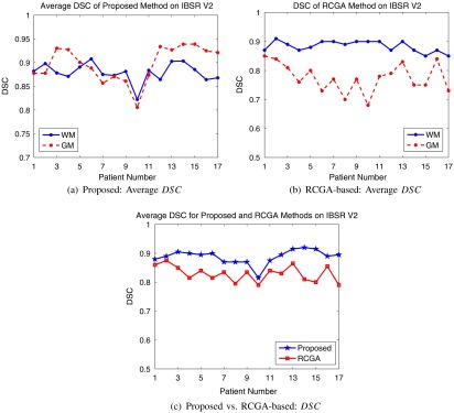
Average DSC for IBSR V2 database using (a) proposed method, (b) model-based approach, and (c) average performance comparison.
The RCGA model–based approach was also employed on the IBSR V2.0 database and validation results are shown in Fig. 11(b). GM segmentation performance is significantly lower than that of WM using the model-based method. A fewer number of GM pixels (versus WM) are used to create the finite mixture models, which could explain the lower performance. These results are compared in Fig. 11(c) by considering the average DSC results from the proposed and RCGA methods [Figs. 11(a) and 11(b)]. The DSC for the model-based approach has reduced performance compared to the proposed approach. Visual results, quantitative measures, and comparison with other methods show the current method is performing well in real, normal MRI with Gaussian distributed noise.
One volume from ISBR V2.0 was not included in the analysis (patient 6). The estimated for this volume is shown in Fig. 12(a). As shown, the gradient operator was unable to differentiate between classes since only a single PVA pulse was localized and it had low amplitude. Comparing the DSC of the proposed work for all volumes as a function of the contrast between classes (the contrast was found by calculating the difference between histogram peaks, normalized by the total range of the image) in Fig. 12(b) demonstrates high performance is achieved for all the images except for patient 6, which is of low contrast ( contrast). This patient demonstrates the breaking point of the algorithm.
Fig. 12.
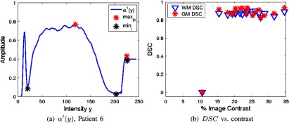
Global edge estimate for IBSR V2.0, patient 6 (a) and DSC as a function of image contrast (b).
4.6. FLAIR Database
The last set of experiments are focused on the FLAIR database. As shown in Table 1, the images in this database have WML pathology and the noise is non-Gaussian.10 Highly accurate segmentation of WML on these images will highlight the benefits of a generalized approach.
To prepare the images for segmentation, brain extraction was applied using the technique in Ref. 14 and bilateral filtering was utilized (as previously described). In brain extracted FLAIR MRI with WML, there are three tissue classes: (1) CSF, (2) brain (WM and GM form a single class25), and (3) WML. Although the tissue classes have different contrast properties than T1-weighted images, no modifications are required to employ the algorithm on the FLAIR MRI with WML.
The results for several images are shown in Fig. 13, where the top row contains original FLAIR MRI with WML manual segmentations, and the bottom row contains the corresponding estimated class membership maps for the WML class, . The interior of the lesions are red (pure) and the boundaries (PVA) receive proportionally less weighting.
Fig. 13.
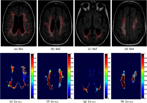
Segmentation of white matter lesion (WML) in fluid attenuation inversion recovery (FLAIR) magnetic resonance images (MRI). Top: original images with manual segmentations. Bottom: corresponding fuzzy membership masks for WML class [].
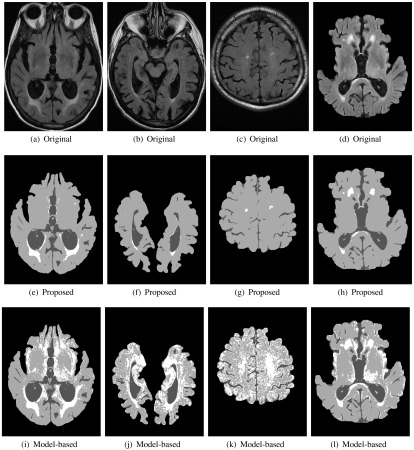
The binary class membership masks are compared to the manual segmentation using the DSC, as shown in Fig. 14(a) for all patients. An average DSC of 0.78 was found for the entire database, indicating good agreement. In Fig. 14(b), performance as a function of lesion volume for the proposed method also shows stable and robust segmentation, despite the variety of lesion loads. A few segmentation results (all tissue classes) are shown in Fig. 15, clearly demonstrating that WML are robustly segmented.
Fig. 14.
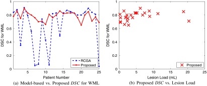
WML segmentation performance for proposed and real-coded genetic algorithm (RCGA)-based technique (a) and DSC as a function of lesion volume for the proposed method (b).
Fig. 15.
Brain tissue segmentation for FLAIR MRI with WML. Top row: original images. Middle: tissue segmentation results from proposed method. Bottom: tissue segmentation results from RCGA-based approach.
The WML segmentation performance of the proposed work is compared to the model-based technique in Fig. 14. The segmentation performance for the model-based technique is low for some images, and moreover, the results are highly variable, suggesting lack of repeatability and reproducibility. The low performance is caused by gross oversegmentation of the WML class as shown by the tissue segmentation masks in Fig. 15. Over segmentation is likely caused by the presence of pathology, as well as the non-normal noise characteristics (non-Gaussian phenomena and pathology, which cannot be handled easily by a model-based technique). This greatly shows the benefits of the current PV fraction estimation and tissue segmentation work.
5. Discussion
The results demonstrate the advantages of the current approach. PV fraction estimation and tissue segmentation performance was high for Gaussian and non-Gaussian noise scenarios, as well as images with pathology. Comparison to model-based approaches shows that it performs exceptionally well, especially in images with non-Gaussian noise properties and pathology. The challenges associated with model-based approaches are mitigated, i.e., intensity distribution of the noise and PVA models do not need to be selected a priori.
There are some challenges with the proposed method. Because the method is based on the gradient, for low contrast-to-noise ratios, there is a decrease in discrimination between PVA and pure regions in (difference between their respective amplitudes is reduced). If the noise and edge information are indistinguishable (as seen by the gradient), it is difficult to recover the edge information. We are currently investigating interesting ways to solve this challenge, for example, by employing a multiscale noise reduction framework that maximizes contrast-to-noise ratios, or other edge metrics that are not dependent on the gradient (i.e., phase congruency or texture-based features). These methods will be incorporated into the overall framework.
Another challenge that stems from low gradient values surrounds the minima/maxima (threshold) detection step. If the contrast is not high enough between classes, the edge strength measure between pure and PVA classes will be small, ultimately reducing the efficacy of the optima detection algorithm. Future works just described will be important for this phase as well.
A common challenge with neuro MRI segmentation approaches is the classification of PVA around the ventricles because PVA in these regions are composed of CSF and WM, which is not usually accounted for in classification problems since they are quantitatively insignificant.6 It forms a special case that has to be handled separately, and although insignificant, we are currently looking at methods to handle this. A ventricle segmentation algorithm is being developed that will be used to impose a spatial constraint in the ventricular region.
The last consideration for future works is the selection of the thresholds. We are currently considering a variety of statistical quantities that explicitly model any uncertainty in this step. Therefore, it will be possible to model the PV fraction, along with an associated confidence interval.
6. Conclusion
The current paper presents a way to model PVA artifacts based on the edge content in the image. It is a generalized and adaptive approach that can be applied to several MRI-weightings for robust PV fraction estimation and brain segmentation. There are no a priori assumptions made about the distributions and no extra imaging modalities are required. It is a stand-alone approach that gives way to complete characterization of the brain tissue’s class membership maps.
The proposed algorithm was employed successfully on simulated and real T1 MRI, as well as FLAIR MRI with WML. Comparison to model-based techniques shows that the edge-based approach outperforms traditional methods for brain segmentation in terms of segmentation performance. This is especially true for images with pathology and non-Gaussian noise characteristics, which are not easily handled by model-based techniques. The proposed methods have great potential for future PV fraction estimation and brain segmentation works.
Biographies
April Khademi is a professor in the Biomedical Engineering Department at the University of Guelph, where she is focused on the research and development of medical image analysis algorithms. Her previous roles include research and product development at PathCore Inc., GE Healthcare, Sunnybrook Hospital, Toronto Rehab Institute, and Khademi Consulting. She received her doctorate in electrical engineering from the University of Toronto. She is a registered professional engineer in the province of Ontario, IEEE senior member, and certified Scrum Master.
Anastasios Venetsanopoulos is a professor of electrical and computer engineering at Ryerson University and a professor emeritus at the University of Toronto. He has authored 10 books, contributed chapters to 30 books, and published over 830 technical papers. He is a fellow of the Engineering Institute of Canada, IEEE, the Canadian Academy of Engineering, and the Royal Society of Canada.
Alan R. Moody has been a faculty member at the University of Toronto since 2003. He was appointed chair of the Department of Medical Imaging in 2012, prior to which he was radiologist in chief at Sunnybrook Health Sciences Centre. He is a clinician scientist within Sunnybrook Research Institute as part of the Schulich Heart Research program. His research interests broadly include the application of imaging for the understanding of disease process.
References
- 1.Leemput K. V., et al. , “A unifying framework for partial volume segmentation of brain MR images,” IEEE Trans. Med. Imaging 22(1), 105–119 (2003). 10.1109/TMI.2002.806587 [DOI] [PubMed] [Google Scholar]
- 2.Ballester M. G., Zisserman A., Brady M., “Estimation of the partial volume effect in MRI,” Med. Image Anal. 6(4), 389–405 (2002). 10.1016/S1361-8415(02)00061-0 [DOI] [PubMed] [Google Scholar]
- 3.Tohka J., Zijdenbos A., Evans A., “Fast and robust parameter estimation for statistical partial volume models in brain MRI,” NeuroImage 23(1), 84–97 (2004). 10.1016/j.neuroimage.2004.05.007 [DOI] [PubMed] [Google Scholar]
- 4.Shattuck D., et al. , “Magnetic resonance image tissue classification using a partial volume model,” NeuroImage 13(5), 856–876 (2001). 10.1006/nimg.2000.0730 [DOI] [PubMed] [Google Scholar]
- 5.Manjon J. V., Tohka J., Robles M., “Improved estimates of partial volume coefficients from noisy brain MRI using spatial context,” Neuroimage 53(2), 480–490 (2010). 10.1016/j.neuroimage.2010.06.046 [DOI] [PubMed] [Google Scholar]
- 6.Cuadra M., et al. , “Comparison and validation of tissue modelization and statistical classification methods in T1-weighted MR brain images,” IEEE Trans. Med. Imaging 24(12), 1548–1565 (2005). 10.1109/TMI.2005.857652 [DOI] [PubMed] [Google Scholar]
- 7.Lin P., et al. , “An efficient automatic framework for segmentation of MRI brain image,” in Int. Conf. on Computer and IT, pp. 896–900, IEEE, China: (2004). [Google Scholar]
- 8.Santago P., Gage H., “Statistical models of partial volume effect,” IEEE Trans. Image Process. 4(11), 1531–1540 (2003). 10.1109/83.469934 [DOI] [PubMed] [Google Scholar]
- 9.Ruan S., et al. , “Brain tissue classification of magnetic resonance images using partial volume modeling,” IEEE Trans. Med. Imaging 19(12), 1179–1187 (2000). 10.1109/42.897810 [DOI] [PubMed] [Google Scholar]
- 10.Khademi A., et al. , “Nonparametric statistical tests for exploration of correlation and nonstationarity in images,” in Int. Conf. on DSP, pp. 1–6, IEEE/EURASIP, Greece: (2009). [Google Scholar]
- 11.Anbeek P., et al. , “Probabilistic segmentation of white matter lesions in MR imaging,” NeuroImage 21(3), 1037–1044 (2004). 10.1016/j.neuroimage.2003.10.012 [DOI] [PubMed] [Google Scholar]
- 12.Zhiqiang L., et al. , “Automated segmentation of white matter lesions in 3D brain MRI, using multivariate pattern classification,” in IEEE ISBI, pp. 307–310, IEEE, USA: (2006). [Google Scholar]
- 13.de Boer R., et al. , “Automatic segmentation of brain tissue and white matter lesions in MRI,” in IEEE ISBI, pp. 652–655, IEEE, USA: (2007). [Google Scholar]
- 14.Khademi A., Venetsanopoulos A., Moody A., “Automatic contrast enhancement of white matter lesions in FLAIR MRI,” in IEEE Int. Symp. on Biomedical Imaging’09, pp. 322–325, IEEE, Argentina: (2009). [Google Scholar]
- 15.Meer P., Georgescu B., “Edge detection with embedded confidence,” IEEE Trans. PAMI 23(12), 1351–1365 (2001). 10.1109/34.977560 [DOI] [Google Scholar]
- 16.Khademi A., Venetsanopoulos A., Moody A., “Edge-based partial volume averaging estimation in FLAIR MRI with white matter lesions,” in Int. Conf. of the IEEE Engineering in Medicine and Biology Society, pp. 6114–6117 (2010). [DOI] [PubMed] [Google Scholar]
- 17.Kvam P. H., Vidakovic B., Nonparametric Statistics with Applications to Science and Engineering, Wiley-Interscience, USA: (2007). [Google Scholar]
- 18.Sled J., Zijdenbos A., Evans A., “A nonparametric method for automatic correction of intensity nonuniformity in MRI data,” IEEE Trans. Med. Imaging 17(1), 87–97 (1998). 10.1109/42.668698 [DOI] [PubMed] [Google Scholar]
- 19.Kwan R.-S., Evans A., Pike G., “An extensible MRI simulator for post-processing evaluation,” Lec. Notes Comput. Sci. 1131, 135–140 (1996). 10.1007/BFb0046929 [DOI] [Google Scholar]
- 20.Collins D., et al. , “Design and construction of a realistic digital brain phantom,” IEEE Trans. Med. Imaging 17(3), 463–468 (1998). 10.1109/42.712135 [DOI] [PubMed] [Google Scholar]
- 21.Fox A., et al. , “Prognostic importance of leukoaraiosis in patients with symptomatic internal carotid artery stenosis,” Stroke 33(6), 1651–1655 (2002). 10.1161/01.STR.0000043820.72323.23 [DOI] [PubMed] [Google Scholar]
- 22.Zou K., et al. , “Statistical validation of image segmentation quality based on a spatial overlap index,” Acad. Radiol. 11(2), 178–189 (2004). 10.1016/S1076-6332(03)00671-8 [DOI] [PMC free article] [PubMed] [Google Scholar]
- 23.Zijdenbos A., et al. , “Morphometric analysis of white matter lesions in MR images: method and validation,” IEEE Trans. Med. Imaging 13(4), 716–724 (1994). 10.1109/42.363096 [DOI] [PubMed] [Google Scholar]
- 24.Tohka J., et al. , “Genetic algorithms for finite mixture model based voxel classification in neuroimaging,” IEEE Trans. Med. Imaging 26(5), 696–711 (2007). 10.1109/TMI.2007.895453 [DOI] [PMC free article] [PubMed] [Google Scholar]
- 25.Jack C., et al. , “FLAIR histogram segmentation for measurement of leukoaraiosis volume,” J. Magn. Reson. Imaging 14(6), 668–676 (2001). 10.1002/(ISSN)1522-2586 [DOI] [PMC free article] [PubMed] [Google Scholar]


