Abstract.
X-ray video fluoroscopy along with two-dimensional–three-dimensional (2D-3D) registration techniques is widely used to study joints in vivo kinematic behaviors. These techniques, however, are generally very sensitive to the initial alignment of the 3-D model. We present an automatic initialization method for 2D-3D registration of medical images. The contour of the knee bone or implant was first automatically extracted from a 2-D x-ray image. Shape descriptors were calculated by normalized elliptical Fourier descriptors to represent the contour shape. The optimal pose was then determined by a hybrid classifier combining -nearest neighbors and support vector machine. The feasibility of the method was first validated on computer synthesized images, with 100% successful estimation for the femur and tibia implants, 92% for the femur and 95% for the tibia. The method was further validated on fluoroscopic x-ray images with all the poses of the testing cases successfully estimated. Finally, the method was evaluated as an initialization of a feature-based 2D-3D registration. The initialized and uninitialized registrations had success rates of 100% and 50%, respectively. The proposed method can be easily utilized for 2D-3D image registration on various medical objects and imaging modalities.
Keywords: pose estimation, 2D-3D registration, support vector machine, computed tomography image, x-ray fluoroscopic image, kinematics
1. Introduction
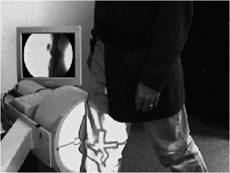
In vivo kinematic analysis using x-ray video fluoroscopy is applied in the evaluation of joint kinematics for both implanted and normal joints.1–3 Figure 1 shows the fluoroscopic imaging in the knee during gait analysis. X-ray video fluoroscopy is a sequence of x-ray images where the metallic implants and the bone appear much darker than the soft tissues surrounding them, allowing for direct observation and analysis of their movement under dynamic and weight bearing conditions. Moreover, fluoroscopy is noninvasive and relatively low risk to the patient. A typical 1-min protocol gives the patient a radiation exposure on the order of 0.6 to 1.8 “rad equivalent man” (rem).3 However, two-dimensional (2-D) fluoroscopic images do not provide three-dimensional (3-D) information. A 3-D CAD/computed tomography (CT)/MRI model is time-consuming (MRI) to generate and exposes patients to more radiation (CT), but it provides 3-D insight and improves visualization of anatomical structures. Therefore, it is necessary to fuse the information of the 2-D images and 3-D volume data by 2D-3D registration.
Fig. 1.
Fluoroscopic imaging in the knee.
In clinical practice, it is desired to keep the number of x-ray fluoroscopic images to a minimum due to cost, acquisition and computation times, and due to radiation exposure constraints. Single plane fluoroscopic imaging has been commonly used to study joint kinematics. Mahfouz et al. illustrated that single plane registration can be achieved with an in-plane accuracy of less than 0.091 mm in translation, with an out-of-plane error of 1.376 mm.2 Different groups have investigated the use of dual fluoroscopy as a method for increasing the out-of-plane registration accuracy.4 However, limited studies have investigated the differences between the two methods using a consistent 2D-3D matching setup.5
The key step in 2D-3D registration is to determine the relationship between the 2-D x-ray image coordinate system and the 3-D model coordinate system. This can be achieved by manual registration of 3-D data to be fitted to the 2-D x-ray image. This method, however, is labor intensive and prone to both inter and intra user variability. An alternative is the use of paired point analytic registration with point data obtained from either skin or bone fiducial markers.6–8 However, skin markers are susceptible to error due to undesired motion between the markers and the underlying bone, and bone markers are invasive, which limits their use. A third method of 2D-3D image registration is to iteratively adapt the unknown pose so as to maximize a similarity measure, which reflects the quality of the registration. A large body of work of 2D-3D registration based on 3-D model registration to radiographs2,9–11 and 3-D kinematic analysis from fluoroscopic images12 has shown satisfactory registration accuracy. Existing 2D-3D registration methods are often limited by a small capture range.13 Due to the nonconvex nature of the similarity measure, such methods can suffer from inaccurate registration results when the initial pose of the 3-D model is outside the capture range. The objective of this paper is to develop a method that provides a large capture range for the 2D-3D registration process by comparing a query shape in a 2-D image with a precomputed training model to determine the initial pose of the 3-D model. The main advantage of the proposed method is the ability to search in a large range of possible solutions making the methods independent of initialization. Moreover, since the pose estimation processes using x-ray fluoroscopy in various planes are independent from each other, our method can be applied to both monoscopic and stereoscopic registrations.
There is a wide variety of published literature on the topic of pose estimation based on template matching.14–17 Khotanzad and Liou15 developed a neural network-based system for recognition and pose estimation of an unoccluded 3-D object from any single 2-D perspective view. The neural network (NN) classifier used in this paper may suffer from multiple local minima and is more prone to over fitting compared with support vector machine (SVM). Unlike NNs, SVMs have a simple geometric interpretation and give a sparse solution. Moreover, the computational complexity of SVMs does not depend on the dimensionality of the input space, which is not the case for NN. Therefore, SVMs often outperform NN in practice where SVMs are less prone to over fitting and yield a global and unique solution.18
Banks and Hodge16 used the template-matching method to measure the pose of knee prostheses by matching the projected silhouette contour of the prosthesis against a library of shapes representing the contour of the object over a range of possible orientations. Hoff et al.17 matched the silhouette of the prostheses components against a library of images to estimate the position and orientation of the component. Both methods directly matched the projected 3-D model image with a template library of implant models. Moreover, they applied the pose estimation to implant models, which has limited shape variation when compared to bone anatomy.
Direct implementation of the template-matching method would require an exhaustive computation time and usage of memory by comparing the distance between the query and the entire training examples dataset. Instead, we used a hybrid classifier to determine the pose of the 3-D model so as to avoid a blanket search. More specifically, the hybrid classifier combines -nearest neighbors (-NN) and SVM, where -NN serves as an attention mechanism, generating an area of interest for the further local search by SVM.19,20 A set of SVMs, each trained to a smaller range of poses, decomposes the pose estimation problem across a large range of poses into a set of subproblems. Thus, the proposed initialization method is more time and space efficient than the conventional direct template-matching methods. Moreover, our method can be easily adapted for various anatomical or implant structures and various imaging modalities.
The rest of the paper is organized as follows. The approaches are described in Sec. 2. Section 3 provides the experiments and their results. Finally, Sec. 4 concludes the paper and gives future prospects.
2. Approach
2.1. Problem Statement
The goal of the proposed method is to estimate the poses of the 3-D model from a single plane fluoroscopic x-ray image based on a precomputed training set of 2-D contours. This method helps kinematics in that it can determine 3-D in vivo and weight bearing kinematics of the knee joint from a single plane fluoroscopic image. It also helps biomechanics in that it determines the orientation of the femur with respect to the tibia so as to determine the forces and torques acting on the knee joints.
Let be the smooth surface of the 3-D model, and denote , to be the corresponding spatial coordinate. Let and be the coordinates and surface in the 3-D world, respectively. We can locate the in the camera reference frame via the transformation such that and the corresponding pointwise expression
| (1) |
where is a rotation matrix , , , and is a translation vector, . is the coordinate of the 3-D model in the 3-D world.
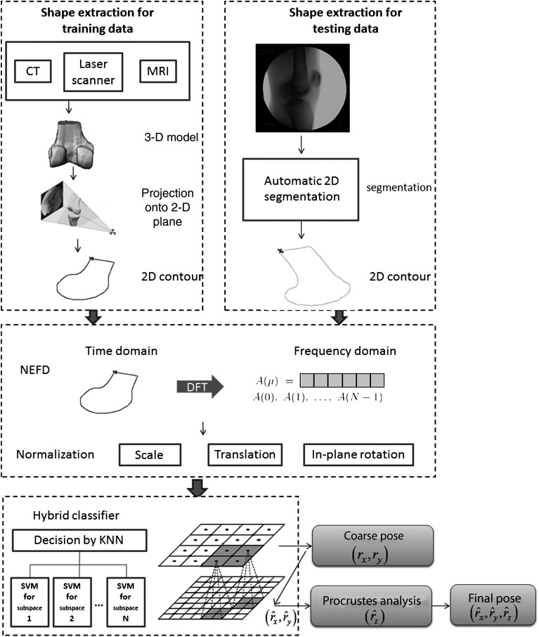
The proposed method consists of three steps: (1) shape extraction to extract the 2-D contour of the object of interest in an x-ray fluoroscopy, (2) shape representation to represent the shape by normalized elliptical Fourier descriptors (NEFDs), (3) classification by a hybrid classifier to estimate the pose of the 3-D model. The system framework is illustrated in Fig. 2.
Fig. 2.
Flow chart of the initialization system.
2.2. Shape Extraction
The contour of the object of interest in the x-ray fluoroscopy is extracted by an active shape model (ASM)-based segmentation algorithm.21 ASM represents the global shape constraints with the dominant shape variation in the training set. The benefit of ASM is that it constrains the search to feasible shapes so that mis-segmentations such as skin segmentation or segmentation of neighboring bones and foreign occlusions can be avoided.
The training data are the contours extracted from the binary images, which are the 3-D surface mesh models projection onto the 2-D plane at different poses, yielding 1887 training contours. The contours are then aligned by finding corresponding points of each contour using statistical atlases, where training contours with a known point distribution are deformed to match one another.22–24 To segment the x-ray image, we start from the average contour in the training dataset; search on the normal profile of each contour point for the greatest gradient; use ASM to constrain the contour to a feasible shape; and then relax the constrained points for the segmented contour. Relaxation is done by a gradient search in the normal profile once again with a half profile length. The contour is closed by drawing a line perpendicular to the major axis of the bone, the direction of which can be represented by the first principal component of the PCA of the contour points. The flowchart of the segmentation algorithm is illustrated in Fig. 3.
Fig. 3.
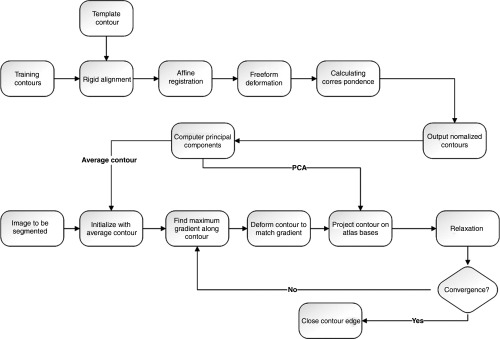
Flow chart of the two-dimensional (2-D) segmentation.
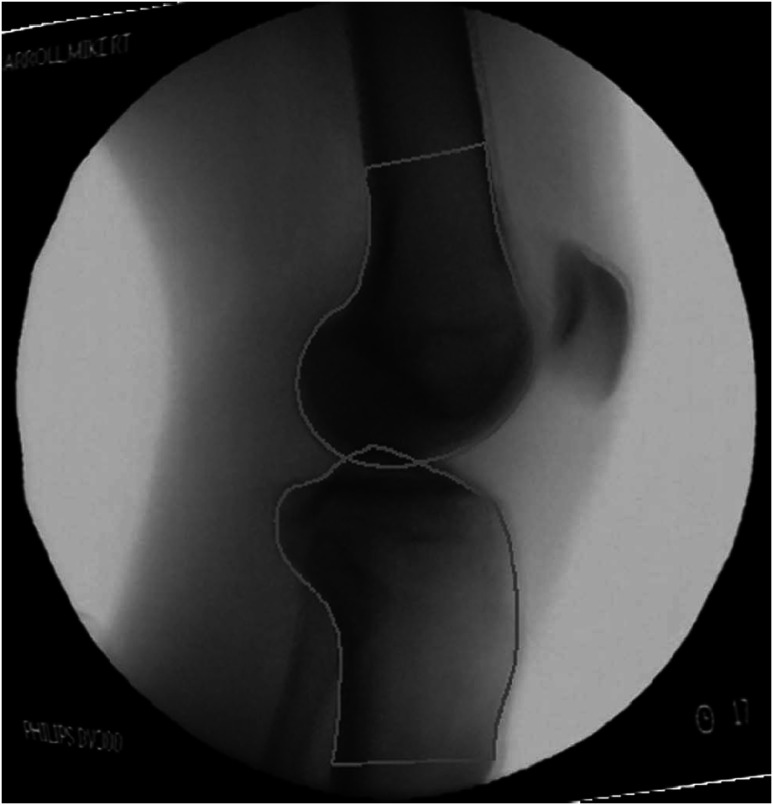
An example of segmentation results is shown in Fig. 4.
Fig. 4.
Segmentation result of femur and tibia in an x-ray image.
2.3. Shape Representation
The shape representation is based on NEFDs developed by Kuhl and Giardina.25 Contours are first normalized by in-plane rotation, translation, and scale. NEFD represents the object shape in a very compact manner and is, therefore, time and space efficient.
2.3.1. Calculate shape descriptors of the contour
The main idea of the elliptical Fourier analysis is to approximate a closed contour as a sum of elliptic harmonics. harmonics are used to identify the closed contour of elements. Four coefficients are used for each harmonic, as given by
| (2) |
| (3) |
| (4) |
| (5) |
where and are the and coordinate values; and represent the projection on the semi major and semi minor axis, and and similarly represent the projection on the semi major and semi minor axis. is the length of the Freeman chain18 of the closed contour, is the length of elements of the chain, and is the number of elements in the chain.
The inverse process allows identification of the closed contour from the coefficients, as given by
| (6) |
| (7) |
where and represent the coordinates of the centroid.
The most significant features of the contour are captured in the lower frequency terms of the Fourier descriptors. Therefore, a more concise representation of the contour can be generated by eliminating the high-frequency terms, as can be seen in Fig. 5(a), where root-mean-square (RMS) error between the reconstructed and the original contour of the femur drops as the number of harmonics increases. Forty harmonics were found to provide accurate representation for the training shapes according to the reconstruction errors shown in Fig. 5(a). The comparison between the original and reconstructed contours from Fourier descriptors is shown in Fig. 5(b).
Fig. 5.
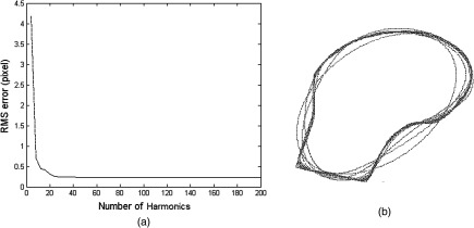
Reconstruction error of NEFD: (a) root-mean-square (RMS) error of reconstructed femur contours with respect to the number of harmonics, (b) reconstructed femur contours are in red with the number of harmonics from 1 to 50. The original contour is in blue.
2.3.2. Normalization
The centroid of the contour is moved to the origin to normalize translation, calculated by
| (8) |
| (9) |
Because the starting point can be chosen randomly and such a choice impacts the coefficient values, it is necessary to have a representation which is invariant to the starting point on the contour. This is achieved by rotating the elliptic coefficients until a shift phase is equal to zero, as given by
| (10) |
where is the phase’s shift from the first major axis. The rotational invariant can be achieved by aligning the major axis of the first harmonic of each image to the axis. The coefficient is normalized by the following equation:
| (11) |
where .
The size invariant is achieved by dividing the length of the semi-major axis, , of the first harmonic:
| (12) |
The invariance of translation, starting point, rotation, and size allows an efficient representation of all the possible shapes.
2.4. Estimate Out-of-Plane Rotation by a Hybrid Classifier
A hybrid classifier was used to estimate the out-of-plane rotation. We consider the estimation of the out-of-plane rotation in the framework of measuring similarities or equivalently distances to the training shapes by a combination of -NN and SVM classifiers. -NN is a nonparametric classifier. An object is classified by a majority vote of its neighbors, with the object being assigned to the class most common among its -NNs.26 While -NN is natural in this kind of problem, it suffers from high variance in the case of limited sampling. Moreover, since the NN classifier uses all the instances in the training set, it is computationally expensive. The alternative is SVM, which models the nonlinear structure of the data by mapping the data onto the high dimensional kernel space and only seeks to model the boundary of the classes. But SVM involves time-consuming optimization and computation of pairwise distances, which makes it difficult to classify a large number of classes. We thus combine -NN and SVM to improve the overall performance.
Since -NN is used for the coarse search, only 5-deg increment instances are used. The Euclidean distance (Ed) is used to measure the similarity between objects and is computed as given below:
| (13) |
where is the Euclidean distance between instance descriptors and , and and are the ’th NEFD of instances and , respectively.
SVM provides a good generalization for pattern classification problems without incorporating problem domain knowledge. Recall that in a two-class SVM classification problem, we want to find a hyper plane that separates the two classes with a maximal margin.27 When it is not possible to linearly separate the two classes, kernel function is used to map the data into a high dimensional space where the data are linearly separable. Given training vectors , , and their label vector such that and the mapping , SVM solves the following optimization problem.
| (14) |
where is a weight vector and is the threshold, maps into a high-dimensional space and is cost coefficient, which represents a balance between the model complexity and the approximation error. When the constraint conditions are infeasible, slack variables can be introduced.
There are different choices of kernels depending on their application at hand. An appropriate selection of the kernel may drastically affect the final classification performance. The radial-basis function (RBF) kernel (or Gaussian kernel) is the most commonly used kernel. Glasner et al. reported a good performance of the RBF kernel28 in the pose estimation problem. We used a Gaussian RBF kernel, .
Penalty parameter in Eq. (14) and in the kernel function are two of the most important parameters. , a regularization parameter, affects the tradeoff between maximizing the margin and minimizing the training error. Both and determine the number of support vectors. Since SVM only models the boundary between each class, the number of support vectors impacts the training time and accuracy. also affects the amplitude of the Gaussian function and therefore affects the generalization ability of SVM.29 The technique used to determine its optimal parameters is a grid search using a cross-validation18,30 that searches the optimal parameters by a coarse grid search with an exponentially growing sequence of (, ) with and followed by a finer grid search to find the one giving the highest accuracy.
Since SVM is a two-class classifier, commonly used methods to extend the two-class classifier into multiclasses include one-against-all method, one against one,31 and directed acyclic graph.32 We use the one-against-one method31 in this paper.
Scaling of the feature vectors is also one of the important factors affecting performance.18 The training set was normalized by scaling it into [0, 1] and then test data were normalized with the same degree of scaling.
2.5. Estimate In-Plane Rotation
Equation (11) in Sec. 2.3.2 provides an approximation of the in-plane rotation by aligning the major axis of the first harmonic of each contour, which is a rough approximation of the real shape. Therefore, a more accurate method is discussed here to determine the in-plane rotation by the angular difference between the best matching contour in the training set and the testing contour through Procrustes analysis.33
| (15) |
Before Procrustes analysis, corresponding points across contours must be established using statistical atlases, as with the corresponding point procedures discussed in Sec. 2.2.
3. Experiments and Results
Three sets of experiments were performed to validate the proposed method. In the first set of experiments (Sec. 3.2), computer simulated images were used to estimate the 3DOF transformation parameters (rotation in , , and axes). A comparison was made among the accuracy of three different classifiers. In the second set of experiments (Sec. 3.3), we further tested the initialization method with x-ray images. In the third set of experiments (Sec. 3.4), the initialization of 6DOF transformation parameters (translation in , , and axes; rotation in , , and axes) was followed by a feature-based 2D-3D registration algorithm. A comparison of performance between initialized and uninitialized registrations was made to test whether the proposed method leads to improved registration.
3.1. Training Data
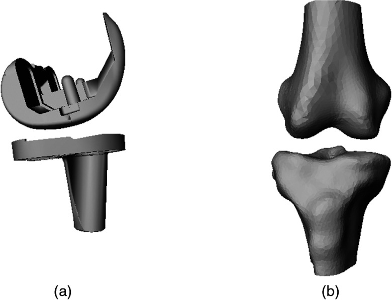
Two datasets were used for training and testing. The first is journey cruciate substituting (BCS) prostheses (Smith and Nephew, Memphis, Tennessee)34 composed of 33 femoral and tibial implants. The implants were laser scanned using a Digibot III machine (DIGI-BOTICS Austin, Texas), which recorded the vertices on the implants’ surface. The second dataset is William M. Bass Donated Skeletal Collection of 100 femurs and tibias from the University of Tennessee’s Anthropology Department. CT scans of the knees were made at levels ranging from 120 mm proximal to the joint to 120 mm distal to the joint. These scans were made at 1–2 mm intervals and the volumetric data of the knee joint were constructed at 0.5 mm interpolation in the transverse plane. Segmentation of the CT-scanned bone was automatically performed by applying a thresholding filter to the slices which isolated the bone from the background. Manual intervention was conducted only when the thresholding filter failed. An example of the 3-D models is depicted in Fig. 6.
Fig. 6.
Three-dimensional (3-D) models of knee bone and implant: (a) 3-D knee implant; (b) 3-D knee bone.
To generate the training set, the 3-D models were rendered on the 2-D plane by a software developed by the authors2 using a 3-D graphic library (Open Inventor, TGS, San Diego, California). A coordinate system was established with the axis pointing to the left, axis pointing upward, and axis pointing out of screen. The impact of the perspective effect on the projected shape was analyzed by comparing the shape variation between two poses with a different translation and fixed rotation during deep knee bending (DKB). The two translational values were set by the first and last poses of the DKB, respectively. As can be seen from Figs. 7(a) and 7(b), neither the shape nor the NEFD varies significantly for these two poses. In addition, in-plane rotation does not lead to any variation in the projected shapes. Therefore, we represent the shape by out-of-plane rotation (around and axes) only, while the translation and in-plane rotation (around axis) are normalized by NEFD.
Fig. 7.
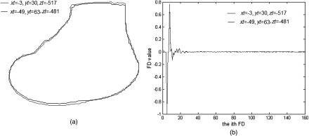
Perspective effect by comparing two poses with the greatest variation in translation and fixed rotation during deep knee bending (DKB): (a) projected shapes; (b) NEFD of the projected shapes.
The 3-D models were rotated in 1-deg increments about the and axes while fixing the position and in-plane rotation. The rotational range is , for the femoral implant; , for the tibial implant; , for the femur; and , for the tibia. At each orientation, the 3-D models were rendered as a binary image so that only the silhouettes are visible.
3.2. Experiments on Simulated Data
Computer simulated data of femoral implant, tibial implant, femur, and tibia were generated by rendering the 3-D models onto the 2-D plane at known poses to validate the accuracy of the estimates provided by the hybrid classifier. The rotational parameters of the testing data were in the same range as training data in the and axes and varying in the range of a 40 deg difference along the axis. The increment was 1 deg for each of the three axial rotations. As an error measurement, we measure the absolute angular difference between the estimated pose and the ground-truth data in each axis. Reported initial mis-registrations leading to successful registrations are in the order of 4–11 mm mTRE13,35 Since a rotation of 1 deg around one of the three axes will lead to an mTRE of 0.8–1.0 mm,36 estimates with an angular error smaller than 4 deg can be safely considered successful. The capture range was defined as the 95% success range as was proposed in Ref. 13.
Ten-fold cross-validations were performed to test the performance of the initialization method. For femoral and tibial implants, 28 patients’ data were used for training and five patients’ data for testing. For femur and tibia, 90 patients’ data were used for training and 10 patients’ data for testing. Each patient’s data contains an equal number of poses as class labels. Table 1 presents the estimates by the initialization method for femoral implant, tibial implant, femur, and tibia. By setting the success threshold as the 4-deg angular difference between estimated and gold standard poses,13,35 100% of the femoral and tibial implants; 92% of the femur and 95% of the tibia estimation were successful.
Table 1.
Root-mean-square (RMS) error of synthetic data experiments with -NN-SVM classifier using 10-fold cross validation (90% patients for training and 10% patients for testing).
| Xr (deg) | Yr (deg) | Zr (deg) | Success rate (%) | |
|---|---|---|---|---|
| Femoral implant | 100 | |||
| Tibia implant | 100 | |||
| Femur | 92 | |||
| Tibia | 95 |
A comparison of performance among single -NN, single SVM, and -NN-SVM is presented in Table 2. The performance improves significantly from single -NN to -NN-SVM. -NN-SVM also outperforms single SVM. Moreover, -NN-SVM is much faster to train because each SVM only involves samples in the local neighborhood, and the number of classes for -NN-SVM is much smaller than that of single SVM.
Table 2.
Average error of tibia pose estimation by -NN, SVM, and -NN-SVM classifier (90% patients for training and 10% patients for testing).
| Xr (deg) | Yr (deg) | Zr (deg) | Success rate (%) | |
|---|---|---|---|---|
| -NN-SVM | 95 | |||
| -NN | 81 | |||
| SVM | 95 |
3.3. Experiments on X-Ray Images
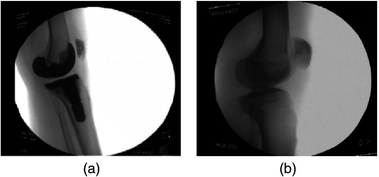
Experiments were performed using x-ray fluoroscopic images acquired using a high-frequency pulsated video fluoroscopy unit. As the largest motion of the knee occurs in the flexion and anteroposterior translation, fluoroscopic imaging was conducted in the sagittal plane. The modern fluoroscopic systems allow video capture at a rate as high as 60 Hz. The fluoroscope is modeled as a perspective projection image formation model, which treats the fluoroscope sensor as consisting of an x-ray point source and a planar phosphor screen upon which the image is formed. The x-ray images had a resolution of . Screenshots of the x-ray images are shown in Fig. 8.
Fig. 8.
Fluoroscopic x-ray images: (a) femoral and tibial implant; (b) femur and tibia.
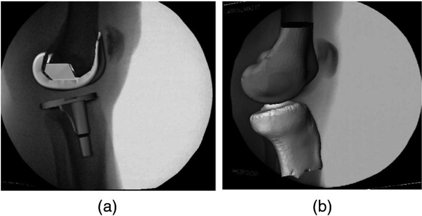
Contours were automatically extracted using the segmentation algorithm mentioned in Sec. 2.2. The overall performance of the method was evaluated by calculating the absolute angular difference between the pose estimated using the proposed method and the ground truth, which is manual fitting. Twenty x-ray images in a series of fluoroscopic images during DKB were used for validation from both datasets. The average error of femoral implant, tibial implant, femur, and tibia is shown in Table 3, where all the prediction poses are within the tolerance angle of 4 deg. An overlay of the estimated 3-D model on the 2-D x-ray image is shown in Fig. 9.
Table 3.
Average error of experiments on x-ray images. Twenty x-ray images for each case.
| Xr(deg) | Yr(deg) | Zr(deg) | |
|---|---|---|---|
| Femoral implant | |||
| Tibial implant | |||
| Femur | |||
| Tibia |
Fig. 9.
Overlay of the estimated 3-D model on the 2-D x-ray image: (a) femoral and tibial implant, (b) femur and tibia.
3.4. Feature-Based 2D-3D Registration Experiments
Experiments were conducted to show the benefit of initialization for 2D-3D registration by comparing the results of initialized and uninitialized registrations. The feature-based 2D-3D registration algorithm was implemented with a normalized cross-correlation similarity measure2 and optimization was performed by simulated annealing. Registrations with a final error smaller than 1 deg were regarded as successes. The uninitialized registration used both the randomly selected starting pose and the middle of the angle range as its initial pose, while the initialized registration used the pose estimated by the proposed initialization method. Translation in the and axes was estimated by the center of the contour. Translation in the axis was estimated by comparing the scale ratio of the testing contour with the one of the known pose.32
A comparison between the result of uninitialized and initialized registrations was made using 10 cases of femoral implant, tibia implant, femur, and tibia, as shown in Table 4. Initialized registration had a success rate of 100%. In contrast, the probability of success for uninitialized registration remained as low as around 50% for the initial pose at the middle of the angle range and around 10% for a randomly selected initial pose.
Table 4.
Results of initialized and uninitialized registrations.
| Average error (deg) | Average error (deg) (obvious failure removed) | Correct registration (%) | Initialization registration | |||
|---|---|---|---|---|---|---|
| Average error (deg) | Correct registration (%) | |||||
| Uninitialized registration (starting point at the middle of the angle range) | ||||||
| Femur implant | Xr | 30 | 100 | |||
| Yr | ||||||
| Zr | ||||||
| Tibia implant | Xr | 40 | 100 | |||
| Yr | ||||||
| Zr | ||||||
| Femur | Xr | 60 | 100 | |||
| Yr | ||||||
| Zr | ||||||
| Tibia | Xr | 50 | 100 | |||
| Yr | ||||||
| Zr | ||||||
| Uninitialized registration (random starting point) | ||||||
| Femur implant | Xr | 10 | ||||
| Yr | ||||||
| Zr | ||||||
| Tibia implant | Xr | 10 | ||||
| Yr | ||||||
| Zr | ||||||
| Femur | Xr | 20 | ||||
| Yr | ||||||
| Zr | ||||||
| Tibia | Xr | 0 | ||||
| Yr | ||||||
| Zr | ||||||
3.5. Speed of the System
The time required for pose estimation was about 5 s on average and the time required for training SVM models was about 15 h. The method was implemented using a combination of C++ and MATLAB® and a 2.7 GHz computer with 8 GB of RAM was used for all of the experiments. Compared with the similar pose estimation study using SVM in the literature,37 whose registration time is 375.3 s and training time is 473.2 s, our method has an obvious advantage in the pose estimation speed. The training of SVM models with our method requires a longer time,37 but it is an offline process thus does not impact the performance of the online pose estimation. The training speed can be improved by parallelizing the training process in the future.
4. Discussions and Conclusions
We developed a pose estimation method as an initialization for 2D-3D registration. More precisely, an ASM-based segmentation method was applied to extract the 2-D contour from -ray images. Normalized elliptical Fourier descriptors were used to represent the shape of the 2-D contour. Then a hybrid classifier integrating -NN and SVM estimated the pose of the 3-D model. Our experimental results demonstrated the reliability of the proposed initialization method for 2D-3D registration.
Automatic initialization is necessary for 2D-3D registration because different initial guesses do not generate a unique solution for the knee position using the automatic 2D-3D registration method.5 The proposed method generates an accurate automatic estimation of the initial pose, leading to improved accuracy in the following 2D-3D registration. Moreover, partial occlusion occurs in fluoroscopic images due to the overlapping between femur and tibia. The proposed method is robust to the occlusion by segmenting the fluoroscopic images based on the data from the statistical atlas. Our method was applied to 2D-3D registration of femur, tibia, femur implant, and tibia implant in this paper, but it can be easily extended for various medical objects and imaging modalities for both monoscopic and stereoscopic registrations. Reliable 2D-3D registration opens up many exciting possibilities such as preoperative planning, intraoperative navigation, and diagnosing purposes by comparing different sources of data such as CT, MRI, and x-ray fluoroscopy images where the visualization of the anatomy is fundamental.
The limitation to the initialization method is that its resolution is limited by the increments of the training data (1 deg in each direction). Therefore, this method is only suitable for initialization purposes. However, it can search in a large range of possible solutions, leading to a capture range as large as the domain of the training data. Moreover, the proposed initialization method does not need any information from the 3-D model during testing. Another limitation is related to mirror and circular symmetry, which leads to similar 2-D projection images at symmetric views. Currently, the proposed method does not address such cases, though this can be solved by including contextual information about the motion of the adjacent elements of the joint to distinguish between symmetric poses. The reason for the choice of angle range in this paper is to cover the domain of the clinical problem being addressed in the current application. It is not method dependent and can be easily expanded to larger ranges for different applications. The training time is also an issue, which can be improved by parallelizing the training process.
Acknowledgments
The authors would like to thank the anonymous reviewers for their helpful comments. The authors would also like to thank Michael Johnson, H. El Dakhakhni, S. M. Zingde, and L. N. Bowers for their help in preparing the paper.
Biographies
Jing Wu received her bachelor’s and master’s degrees in material science and engineering (MSE) from Shanghai Jiao Tong University in 2005 and 2008. Currently, she is working toward her PhD in biomedical engineering at the University of Tennessee. Her current research interests include medical imaging, computer vision, signal processing, machine learning, and optimization.
Emam E. Abdel Fatah received his bachelor’s degree in biomedical engineering from Cairo University and his PhD in biomedical engineering from the University of Tennessee. Currently, he is an assistant professor at the Institute of Biomedical Engineering iBME at the University of Tennessee. He has published various articles in distinguished international journals, with over 50 abstracts and short papers accepted for publication at international conferences. His research interests include medical imaging, machine learning, biomechanics, anthropology, and pervasive computing.
Mohamed R. Mahfouz is a professor in the Mechanical, Aerospace, and Biomedical Engineering Departments at the University of Tennessee (UT). He was awarded the prestigious titles of research fellow by UT’s College of Engineering and chair, career development professor in 2007 and 2011. Currently, he is chair of the Institute of Biomedical Engineering at UT. He has published 150+ journal articles in distinguished journals, with 400+ abstracts and short papers, and has given 40+ guest lectureships worldwide.
References
- 1.Stiehl J. B., et al. , “Fluoroscopic analysis of kinematics after posteriorcruciate-retaining knee arthroplasty,” J. Bone Joint Surg. Br. 77(6), 884–889 (1995). [PubMed] [Google Scholar]
- 2.Mahfouz M. R., et al. , “A robust method for registration of three-dimensional knee implant models to two-dimensional fluoroscopy images,” IEEE Trans. Med. Imaging. 22, 1561–1574 (2003). 10.1109/TMI.2003.820027 [DOI] [PubMed] [Google Scholar]
- 3.Adrija Sharma R. D. K., Mahfouz M. R., “In vivo kinematics evaluation in flexion of patients implanted with primary TKA,” Tech. Knee Surg. 10(2), 66–72 (2011). 10.1097/BTK.0b013e31821cabb2 [DOI] [Google Scholar]
- 4.Li G., Van de Velde S. K., Bingham J. T., “Validation of a non-invasive fluoroscopic imaging technique for the measurement of dynamic knee joint motion,” J. Biomech. 41, 1616–1622 (2008). 10.1016/j.jbiomech.2008.01.034 [DOI] [PubMed] [Google Scholar]
- 5.Zhu Z. L., Li G. A., “An automatic 2D-3D image matching method for reproducing spatial knee joint positions using single or dual fluoroscopic images,” Comput. Methods Biomech. Biomed. Eng. 15, 1245–1256 (2012). 10.1080/10255842.2011.597387 [DOI] [PMC free article] [PubMed] [Google Scholar]
- 6.Miao S., Lucas J., Liao R., “Automatic pose initialization for accurate 2-D/3-D registration applied to abdominal aortic aneurysm endovascular repair,” in Medical Imaging 2012: Image-Guided Procedures, Robotic Interventions, and Modeling, Holmes D. R., Wong K. H., Eds., Vol. 8316, (2012). [Google Scholar]
- 7.Antonsson E. K., Mann R. W., “Automatic 6-DOF kinematic trajectory acquisition and analysis,” J. Dyn. Syst. Meas. Control 111, 31–39 (1989). 10.1115/1.3153016 [DOI] [Google Scholar]
- 8.Sati M., et al. , “Quantitative assessment of skin-bone movement at the knee,” Knee 3, 121–138, (1996). 10.1016/0968-0160(96)00210-4 [DOI] [Google Scholar]
- 9.Baka N., et al. , “Statistical shape model-based femur kinematics from biplane fluoroscopy,” IEEE Trans. Med. Imaging 31, 1573–1583 (2012). 10.1109/TMI.2012.2195783 [DOI] [PubMed] [Google Scholar]
- 10.Zheng G., “Unifying energy minimization and mutual information maximization for robust 2D/3D registration of x-ray and CT images,” in Proc. Pattern Recognition, vol. 4713, Hamprecht F. A., Schnorr C., Jahne B., Eds., pp. 547–557 (2007). [Google Scholar]
- 11.Bifulco P., et al. , “2D-3D registration of CT vertebra volume to fluoroscopy projection: a calibration model assessment,” EURASIP J. Adv. Signal Process. 2010, 1–8 (2010). 10.1155/2010/806094 [DOI] [Google Scholar]
- 12.Dennis D. A., et al. , “In vivo determination of normal and anterior cruciate ligament-deficient knee kinematics,” J. Biomech. 38, 241–253 (2005). 10.1016/j.jbiomech.2004.02.042 [DOI] [PubMed] [Google Scholar]
- 13.van de Kraats E. B., et al. , “Standardized evaluation methodology for 2-D-3-D registration,” IEEE Trans. Med. Imaging 24, 1177–1189 (2005). 10.1109/TMI.2005.853240 [DOI] [PubMed] [Google Scholar]
- 14.Thayananthan A., “Template-based pose estimation and tracking of 3D hand motion,” Doctor of Philosophy, University of Cambridge (2005).
- 15.Khotanzad A., Liou J. J. H., “Recognition and pose estimation of unoccluded three-dimensional objects from a two-dimensional perspective view by banks of neural networks,” IEEE Trans. Neural Netw. 7, 897–906 (1996). 10.1109/72.508933 [DOI] [PubMed] [Google Scholar]
- 16.Banks S. A., Hodge W. A., “Accurate measurement of three-dimensional knee replacement kinematics using single-plane fluoroscopy,” IEEE Trans. Biomed. Eng. 43, 638–649 (1996). 10.1109/10.495283 [DOI] [PubMed] [Google Scholar]
- 17.Hoff W. A., et al. , “Three-dimensional determination of femoral-tibial contact positions under in vivo conditions using fluoroscopy,” Clin. Biomech. 13, 455–472 (1998). 10.1016/S0268-0033(98)00009-6 [DOI] [PubMed] [Google Scholar]
- 18.Chang C.-C., Lin C.-J., “LIBSVM: a library for support vector machine,” Acm Trans. Intel. Syst. Technol. 2(3), 1–27 (2001). [Google Scholar]
- 19.Aizerman M. A., Braverma E. M., Rozonoer L. I., “Theoretical foundations of potential function method in pattern recognition learning,” Autom. Remote Control 25(6), 821–837 (1964). [Google Scholar]
- 20.Cortes V. V. C., “Support-vector networks,” Mach. Learn. 20(3), 273–297 (1995). 10.1023/A:1022627411411 [DOI] [Google Scholar]
- 21.Cootes T. F., et al. , “Active shape models: their training and application,” Comput. Vis. Image Und. 61, 38–59 (1995). 10.1006/cviu.1995.1004 [DOI] [Google Scholar]
- 22.Abdel Fatah E. E., et al. , “Improving sex estimation from crania using a novel three-dimensional quantitative method,” J. Forensic Sci. 59, 590–600 (2014). 10.1111/1556-4029.12379 [DOI] [PubMed] [Google Scholar]
- 23.Mahfouz M. R., et al. , “Automatic methods for characterization of sexual dimorphism of adult femora: distal femur,” Comput. Methods Biomech. Biomed. Eng. 10, 447–456 (2007). 10.1080/10255840701552093 [DOI] [PubMed] [Google Scholar]
- 24.Mahfouz M., et al. , “Patella sex determination by 3D statistical shape models and nonlinear classifiers,” Forensic Sci. Int. 173, 161–170 (2007). 10.1016/j.forsciint.2007.02.024 [DOI] [PubMed] [Google Scholar]
- 25.Kuhl F. P., Giardina C. R., “Elliptic Fourier features of a closed contour,” Comput. Graph. Image Process. 18, 236–258 (1982). 10.1016/0146-664X(82)90034-X [DOI] [Google Scholar]
- 26.Altman N. S., “An introduction to kernel and nearest-neighbor nonparametric regression,” Am. Stat. 46(3), 175–185 (1992). 10.1080/00031305.1992.10475879 [DOI] [Google Scholar]
- 27.Scholkopf B., Smola A., Learning with Kernels, MIT Press, Cambridge, Massachusetts: (2002). [Google Scholar]
- 28.Glasner D., et al. , “Viewpoint-aware object detection and continuous pose estimation,” Image Vis. Comput. 30, 923–933 (2012). 10.1016/j.imavis.2012.09.006 [DOI] [Google Scholar]
- 29.Zhao C. Y., et al. , “Prediction of milk/plasma drug concentration (MIP) ratio using support vector machine (SVM) method,” Pharm. Res. 23, 41–48 (2006). 10.1007/s11095-005-8716-4 [DOI] [PubMed] [Google Scholar]
- 30.Fei Z., Tiyip T., “A method of soil salinization information extraction with SVM classification based on ICA and texture features,” Agri. Sci. Technol. 12(7), 1046–1049+1074 (2011). [Google Scholar]
- 31.Knerr S., Personnaz L., Dreyfus G., “Single-layer learning revisited: a stepwise procedure for building and training a neural network,” in Neurocomputing: Algorithms, Architectures and Applications, Souli F., Ed., Vol. F68, Springer-Verlag, pp. 41–50 (1990). [Google Scholar]
- 32.Chen S. C., Murphy R. F., “A graphical model approach to automated classification of protein subcellular location patterns in multicell images,” Bmc Bioinf. 7(1), 90 (2006). 10.1186/1471-2105-7-90 [DOI] [PMC free article] [PubMed] [Google Scholar]
- 33.Dryden I. L., Mardia K. V., Statistical Shape Analysis, Wiley, Chichester: (1998). [Google Scholar]
- 34.Victor J., et al. , “In vivo kinematics after a cruciate-substituting TKA,” Clini. Orthop. Relat. Res. 468, 807–814 (2010). 10.1007/s11999-009-1072-7 [DOI] [PMC free article] [PubMed] [Google Scholar]
- 35.Fitzpatrick J. M., West J. B., Maurer C. R., “Predicting error in rigid-body point-based registration,” IEEE Trans. Med. Imaging 17, 694–702 (1998). 10.1109/42.736021 [DOI] [PubMed] [Google Scholar]
- 36.van der Bom M. J., et al. , “Robust initialization of 2D-3D image registration using the projection-slice theorem and phase correlation,” Med. Phys. 37, 1884–1892 (2010). 10.1118/1.3366252 [DOI] [PubMed] [Google Scholar]
- 37.Qi W. Y., et al. , “Effective 2D-3D medical image registration using support vector machine,” in 2008 30th Annual Int. Conf. Proc. IEEE Eng. Med. Biol. Soc., Vol. 1–8, pp. 5386–5389 (2008). [DOI] [PubMed] [Google Scholar]


