Improving efficiency in clinical trials using auxiliary information; Application of a multi-state cure model

Summary

In clinical trials, an intermediate marker measured after randomization can often provide early information about the treatment effect on the final outcome of interest. We explore the use of recurrence time as an auxiliary variable for estimating the treatment effect on overall survival in phase three randomized trials of colon cancer. A multi-state model with an incorporated cured fraction for recurrence is used to jointly model time to recurrence and time to death. We explore different ways in which the information about recurrence time and the assumptions in the model can lead to improved efficiency. Estimates of overall survival and disease-free survival can be derived directly from the model with efficiency gains obtained as compared to Kaplan-Meier estimates. Alternatively, efficiency gains can be achieved by using the model in a weaker way in a multiple imputation procedure which imputes death times for censored subjects. By using the joint model, recurrence is used as an auxiliary variable in predicting survival times. We demonstrate the potential use of the proposed methods in shortening the length of a trial and reducing sample sizes.

1. Introduction

There is much interest in intermediate outcome variables as either surrogate endpoints (Alonso and Molenberghs, 2008; Buyse and Molenberghs, 1998; Wang and Taylor, 2003) or auxiliary variables for the true outcome of interest in randomized clinical trials. A surrogate endpoint is one that is intended to replace the true outcome of interest in evaluating therapy while an auxiliary variable is one that is intended to be used to improve the efficiency of the analysis of the true endpoint. For clinical trials in locally advanced colon cancer, overall survival has traditionally been considered the definitive endpoint. However, the earlier endpoint of disease-free survival, defined as the time to the first event of either death or cancer recurrence, has been determined to be a good surrogate for overall survival (Chen, et al. 1998; Sargent, et al. 2005). Here, we explore an alternative use of recurrence time in colon cancer trials, that of an auxiliary variable which can be used to shorten the length of a trial and improve the efficiency of the analysis of overall survival.

A variety of methods have been explored to utilize intermediate variables to improve the efficiency of the analysis of the final endpoint (Finkelstein and Schoenfeld, 1994; Fleming, et al 1994; Kosorok and Fleming, 1993; Lagakos, 1977). Cook and Lawless (2001) used a three-stage model for a time-to-event intermediate marker and true endpoint and showed that substantial gains in efficiency are possible with parametric models that assume a close structural relationship between the intermediate variable and true endpoint. Li, et al. (2011) used a parametric model formulation to demonstrate an increase in efficiency in the analysis of the true endpoint when plausible prior assumptions were placed on certain model parameters. Broglio and Berry (2009) partitioned overall survival time into two parts, progression-free survival and survival post-progression and discussed the benefits of considering the treatment effects on each of these endpoints separately. In the scenario of an auxiliary longitudinal variable and a censored event time of interest, Faucett, et al. (2002) developed an approach for using auxiliary variables to recover information from censored observations in survival analysis using a joint longitudinal and survival model and a multiple imputation procedure for the event times of censored subjects. Conlon, et al. (2011) considered the use of recurrence time as an auxiliary variable for overall survival by building separate models for time-to-recurrence and time-to-death. A cure model was used to model time to recurrence and a proportional hazards model with a Weibull baseline hazard function that included recurrence as a time-dependent covariate was used to model death. The model for time-to-death was then used in a multiple imputation procedure to impute death times for censored subjects, and these new data were used in the primary analyses on overall survival. Using some of the same data as considered in the current paper, they showed modest but consistent gains in efficiency by using the auxiliary information in recurrence times. Here, we extend this idea by building a joint multi-state model for recurrence and death with an incorporated cured fraction for the recurrence event. This model is then used to impute death times for censored subjects with the goal of improving the efficiency of the analysis on overall survival. The model proposed here, while more complex and more difficult to estimate than the model used by Conlon, et al. (2011), utilizes the full data likelihood rather than a two-step procedure and offers the potential for larger gains in efficiency.

The model that we use for the recurrence and death events is a multi-state model with a latent cured fraction, described in detail in Conlon, et al. (2014) and depicted graphically in Figure 1. This model is motivated by the disease process in colon cancer clinical trials. In the randomized trials that we consider there are two outcomes of interest, recurrence and death, where death can occur either without prior recurrence or after a recurrence. Additionally, a proportion of subjects censored for recurrence may be cured of disease, and will therefore never experience a recurrence. For subjects censored for recurrence who are not cured of disease, their recurrence time will occur after their censoring time and is therefore unobserved. The primary focus of this paper is exploring the potential for efficiency gains by using the model in different ways, thus only a brief description of the model itself will be given here. Full details of the model, including an assessment of its fit are given in Conlon, et al. (2014). The model includes four hazards for transitioning between the four disease states which include: alive and cured of disease, alive and uncured of disease, alive with recurrence and death. Transitions between these states are described by the multi-state model. The hazard of each transition is modeled using a proportional hazard model with a Weibull baseline hazard function. As we are interested in the gap time between recurrence time and death time, the multi-state model that we used is a semi-Markov model, which sets the clock back to 0 upon entry into a new state. The cured fraction is modeled using the mixture model formulation of the cure model, with the probability of cure specified by a logistic model.

Figure 1.

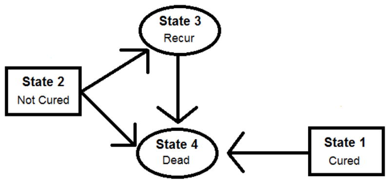
Multi-state cure model structure: observable states are represented by ovals and latent states are represented by rectangles. Latent states are assumed to be determined at time 0 as a result of treatment. Arrows represent transitions that can be made between states.

The proposed parametric model itself can be used to obtain efficiency gains relative to Kaplan-Meier estimates in the estimation of quantities of interest such as the difference in five year overall survival or three year disease-free survival rates between treatment arms. Once parameter estimates from the model are obtained, the estimated five year survival and three year disease-free survival can be computed from the model, which we refer to as the model derived quantities, with the point estimates and standard errors compared to the respective Kaplan-Meier estimates. The model derived quantities utilize the parametric assumptions of the model as well as recurrence information to achieve efficiency gains.

In an alternative way to gain efficiency in the estimation of overall survival, the model can be used in a weaker way by utilizing it in a multiple imputation procedure to impute death times for censored subjects. Patients who are alive at the time of their last follow-up are right censored for death, which we consider as a form of missing data. A patient’s recurrence status prior to their censoring time is usually known, and those who experience a recurrence are likely to die sooner than those who are recurrence free. Therefore, the information on a patient’s recurrence time and status may be useful in predicting their survival time.

The remainder of the paper is organized as follows: Section 2 describes the colon cancer clinical trial data that the proposed methods are applied to, and Section 3 describes the proposed multi-state cure model. In Section 4, ways in which efficiency can be gained from the model are explored. Section 5 provides details of the imputation procedure. In Section 6, we demonstrate the use of the proposed methods is shortening the length of a trial and simulation results are provided in Section 7. Section 8 concludes with a discussion.

2. Description of data from colon cancer clinical trials

We consider data from 12 randomized phase III adjuvant trials of locally advanced colon cancer, ten of which are included in the Sargent, et al. (2005) publication. As these 12 trials are fully described and modeled using the multi-state cure model in Conlon, et al. (2014), we focus on only two of these trials (Trials 3 and 9) in the current paper. Details of the remaining 10 trials can be found in Web Appendix A. In the first trial that we consider (Trial 3), subjects were randomized to the control group of surgery alone or to the treatment group of surgery plus chemotherapy. In the second trial (Trial 9), subjects were randomized to receive surgery plus one of two different types of chemotherapy. Trial 3 (Trial 9) comprised a total of 926 (2,077) subjects, with 457 (1,386) subjects randomized to the treatment arm and 469 (691) randomized to the control arm. Trial 3 (Trial 9) had 377 (605) recurrences and 422 (724) deaths. The primary goal of both trials was to compare overall survival between the treatment arms. Additional covariates measured at baseline include age and cancer stage. The ages of subjects in Trial 3 (Trial 9) ranged from 18 to 90 years (15 to 70 years) with a mean of 60 years (57 years). In Trial 3 (Trial 9), 66% (59%) of the subjects had stage 3 disease. The remaining subjects in both trials had stage 2 disease.

We censored subjects for both death and recurrence at eight years after the last subject accrual in both trials. As the cure model is applied to the recurrence event and most recurrences occur within five years, censoring the data eight years after the last accrual (after which the original data was less reliable) still provides long enough follow-up of the recurrence event to allow a cure model to be fit to the data. Subjects were followed with cancer recurrences and deaths recorded as they occurred, resulting in two, potentially censored, event times of interest. The censoring times for these events is not always the same, as while obtaining recurrence status requires active follow-up, a death status can be obtained through other means. No subjects in Trial 3 were censored for recurrence prior to being censored for death, while 8.9% of subjects were censored for recurrence prior to being censored for death in Trial 9. Most recurrences happened within a fixed time frame of about five years, which is characteristic of data in which there is a cured group. Of the 538 (1,280) subjects at risk for recurrence after five years in Trial 3 (Trial 9), only 23 (29) recurred after that time. Kaplan-Meier plots of time-to-recurrence (Conlon, et al., 2014) show a clear leveling off, indicating that this is data for which a cure model is appropriate. Subjects who experienced a recurrence tended to die soon after. Of the 377 (605) subjects who recurred in Trial 3 (Trial 9), 315 (506) were observed to die within 3 years.

3. Multi-state cure model and MCMC estimation

The model we will be utilizing is exactly the same as given in Conlon et al. (2014), so will only be briefly described here. The model jointly considers recurrence and death as well as a latent indicator for cured for recurrence. Deaths can occur either without a prior recurrence or following a recurrence. The deaths that occur without a prior recurrence are known not to be directly due to the regrowth of the cancer, while deaths following a recurrence may be due to the cancer or other causes. Cause of death is not available and not considered in our models. We use the multi-state model to model four transition intensities between four disease states, as illustrated in Figure 1.

3.1 Notation and multi-state cure model specifications

For each trial, let C_ir and T_ir be the censoring and event times for recurrence and let C_id and T_id be the censoring and event times for death for the ith subject, i = 1, …n. Then Y_ir = min(C_ir, T_ir) and the event indicator for recurrence, δ_ir = I(T_ir ≤ C_ir), and Y_id = min(C_id, T_id) and the indicator for death, δ_id = I(T_id ≤ C_id), are observed. Let Z_i, S_i and A_i represent the baseline values of treatment group, cancer stage and age for each subject.

Both the models for the time of entry into each state and for the probability of cure, p, can depend on covariates. The multi-state process is characterized through transition intensities λ_kj(t), which is the instantaneous hazard of entering State j, given that the previous state occupied was State k. From this hazard, we can define the survival distributions for each transient state and their probability density functions.

We use a proportional hazards model with a Weibull baseline hazard function to model the distribution of waiting times. Specifically, the hazard for subject i transitioning to state j, conditional on being in state k just prior to time t_i and on their latent cured status and covariate values is given by ${\lambda }_{kj}(t_i;{\mathbf{X}}_i)=\left(\frac{{\rho }_{kj}}{{\lambda }_{kj}}\right){\left(\frac{t_i}{{\lambda }_{kj}}\right)}^{{\rho }_{kj}-1}\mathit{exp}({\mathbf{X}}_i{\beta }_{kj})$ and the probability of being cured, p, is modeled using a logistic link function given by $p_i=\frac{\mathit{exp}({\mathbf{X}}_i\gamma )}{1+\mathit{exp}({\mathbf{X}}_{\mathbf{i}}\gamma )}$ For transitions 1 → 4 and 2 → 4, t_i is a death time. For transition 2 → 3, t_i is a recurrence time and for transition 3 → 4, t_i is the gap time between entry into the recurred state and death. X_i represents a vector of subject-specific covariates. For transitions 1 → 4, 2 → 3, and 2 → 4, and for the probability of cure we include the covariates age, treatment group and stage. For transition 3 → 4, we include the recurrence time as an additional covariate. There are six distinct types of subjects who contribute to the likelihood: those who recur and are either alive or dead, those who are censored for recurrence at either their death time or censoring time for death, and those who are censored for recurrence prior to either their death time or censoring time for death. The equations for each of these likelihood contributions can be found in Conlon, et al. (2014).

3.2 Details of the MCMC estimation procedure of multi-state cure model parameters

We use an MCMC technique to estimate the parameters of the model. There are a total of 25 parameters to estimate for each of the trials, which includes a shape (ρ) and scale (λ) parameter from the Weibull model for each of the hazard rates, covariate effects for each of the hazard models and covariate effects in the logistic model for the probability of cure. We place informative Normal(0, 0.25²) priors on the treatment and stage coefficients in transition 1 → 4 as treatment group and cancer stage are unlikely to have a large effect on the hazard of death in patients who are cured of disease. We place Normal(0, 2²) priors on the log(λ)’s and gamma priors with mean 1 and standard deviation 0.6 on the ρ’s. Normal(0,1) priors are placed on all of the remaining covariate coefficients in the hazard models and in the logistic model. The impact of these mildly informative priors on the estimation of model parameters is evaluated in Conlon, et al. (2014), where the priors used in the current paper were found to result in less biased estimates than those obtained under less informative priors. A Metropolis-Hastings algorithm is used to obtain parameter draws from the posterior distribution. Details of the algorithm can be found in Conlon, et al. (2014). For each parameter, we obtain 5000 draws from the posterior distribution.

A thorough assessment of the goodness-of-fit was undertaken in Conlon, et al. (2014), through the use of Cox-Snell and deviance residuals, comparisons of predicted versus observed time-to-event distributions, and comparisons of the DIC value of the proposed model with alternative models. We demonstrated that the model gives a good fit, as well as providing parameter estimates which were scientifically plausible, and largely consistent across the 12 trials. Parameter estimates for each of the 12 trials can be found in Conlon, et al. (2014).

4. Application of the model for efficiency gains: Model-based estimates

Typical analyses of the treatment effect on overall survival would be log-rank tests, hazard ratio estimates using Cox models and estimates of differences in survival at specific times points. Since the multi-state cure model does not result in the proportional hazards assumption being satisfied for time-to-death, we focus on estimates of overall survival. Once parameter estimates have been obtained, the model can be used to estimate the difference in five year overall survival (OS) between the two treatment arms. The point estimate can be compared with the Kaplan-Meier estimate to check the model fit and the posterior standard deviation can be compared with the standard error of the Kaplan-Meier estimate to assess gains in efficiency through use of the multi-state cure model.

Let $S_1(t)=\mathit{exp}\left(-{\int }_0^t{\lambda }_{14}(u)du\right)$ and $S_2(t)=\mathit{exp}\left(-{\int }_0^t{\lambda }_{23}(u)du-{\int }_0^t{\lambda }_{24}(u)du\right)$, which are the survival distributions for remaining in State 1 or State 2, respectively. For each subject the five year OS probability is $P(T_i>5\mid {\mathbf{X}}_i,\theta )=p_i{S}_1(5)+(1-p_i)S_2(5)+(1-p_i){\int }_0^5{S}_2(u){\lambda }_{23}(u)\mathit{exp}\left(-{\int }_0^{5-u}{\lambda }_{34}(v)dv\right)$, where θ is the vector of parameter values. This probability is calculated separately for subjects in each treatment arm, and then averaged across the stage and age covariate values for each subject and across all posterior parameter draws to obtain a population estimate.

Similarly, three year disease free survival (DFS) can be calculated from the model and compared to the three year Kaplan-Meier DFS estimate to assess efficiency gains from using the proposed model at the earlier time point. For each subject, three year DFS is calculated as P(DFS_i > 3|X_i, θ) = p_iS₁(3) + (1 − p_i)S₂(3). This probability is then averaged across covariate values for each subject and across all parameter draws. Using the above model derived quantities, we estimate the treatment effect for these two separate endpoints of interest. For trials such as these in locally advanced colon cancer, five year OS is often considered the definitive endpoint. In this setting, three year DFS has been determined to be a valid surrogate marker for five year OS. Therefore, there is interest in the treatment effect estimate at both of these endpoints. In Table 1, the “Full Follow-up” column provides the Kaplan-Meier estimates and standard errors and multi-state model estimates and posterior standard deviations for five year OS and three year DFS. Both the five year OS estimate and the three year DFS estimate from the multi-state model are similar to the Kaplan-Meier estimates, with moderate gains in efficiency obtained by using the multi-state model, as seen by the smaller posterior standard deviations. Five year OS and three year DFS estimates obtained from the multi-state model for the other 10 colon cancer trials can be found in Web Appendix B.

Table 1.

Illustration of efficiency gains using multistate-cure model-based estimates. Kaplan-Meier treatment effect estimates (standard errors) and multi-state model estimates (posterior standard deviations) for the difference in 5 year overall survival (ΔS(5)) and 3 year disease free survival (ΔDFS(3)) between treatment arms for the full follow-up and artificially censored (reduced follow-up) data from 2 colon cancer clinical trials

		ΔS(5)*		ΔDFS(3)**
		Full Follow-up	Reduced Follow-up	Full Follow-up	Reduced Follow-up
Trial 3	Kaplan-Meier	0.074 (0.031)	0.115 (0.080)	0.110 (0.031)	0.210 (0.086)
	Multi-state Model	0.072 (0.026)	0.050 (0.028)	0.113 (0.027)	0.121 (0.030)
Trial 9	Kaplan-Meier	0.034 (0.021)	0.050 (0.026)	0.032 (0.021)	0.042 (0.022)
	Multi-state Model	0.034 (0.018)	0.028 (0.018)	0.039 (0.019)	0.042 (0.020)

^*ΔS(5) = P(T > 5|Z_i = 1) – P(T > 5|Z_i = 0),

^**ΔDFS(3) = P(DFS > 3|Z_i = 1) – P(DFS > 3|Z_i = 0) where T is survival time, DFS is disease free survival time and Z is a binary treatment indicator.

5. Application of the model for efficiency gains: Multiple Imputation

An alternative way that the multi-state cure model can be used to improve efficiency in the estimation of overall survival is through a multiple imputation strategy that imputes death times for subjects who are censored for death. Using the proposed model in a multiple imputation procedure is a less model-dependent approach than the estimation procedure in Section 4 because the model is only used to aid in imputation of the missing data, with the end analysis being of the original data augmented by the imputed data. The multiple imputation approach could be used to improve efficiency of the analysis of overall survival or to shorten the length of a clinical trial while still keeping the primary endpoint of overall survival.

The imputation procedure is performed as follows. For each set of parameter draws, θ, from the posterior distribution, we impute a death time from the residual survival distribution, P(T_id > Y_id + a_i|T_id > Y_id, δ_id = 0, Y_ir, δ_ir, X_i, θ), for each censored subject. Specifically, we set this function equal to a w ~ U(0, 1) random variable and solve for a_i, the imputed time to death after Y_id for each censored subject. For subjects with a recurrence prior to their censoring time (δ_ir = 1), we solve $w=\mathit{exp}\left(-{\int }_{Y_{id}-Y_{ir}}^{Y_{id}+a_i-Y_{ir}}{\lambda }_{34}(u)du\right)$ for a_i. For subjects censored for recurrence (δ_ir = 0) we first calculate their probability of being cured of disease by drawing a Bernoulli(c_i) random variable, where c_i is the probability of being cured of disease, given Y_id, Y_ir, X_i and the current parameter draws. For subjects censored for recurrence at Y_id, c_i is given by $c_i=\frac{p_i{\lambda }_{14}{(Y_{id})}^{{\delta }_{id}}{S}_1(Y_{id})}{p_i{\lambda }_{14}{(Y_{id})}^{{\delta }_{id}}{S}_1(Y_{id})+(1-p_i){\lambda }_{24}{(Y_{id})}^{{\delta }_{id}}{S}_2(Y_{id})}$ and for those censored for recurrence at Y_ir prior to Y_id, c_i is given by $c_i=\frac{p_i{\lambda }_{14}{(Y_{id})}^{{\delta }_{id}}{S}_1(Y_{id})}{p_i{\lambda }_{14}{(Y_{id})}^{{\delta }_{id}}{S}_1(Y_{id})+(1-p_i){\lambda }_{24}{(Y_{id})}^{{\delta }_{id}}{S}_2(Y_{id})+(1-p_i)B}$, where $B={\int }_{Y_{ir}}^{Y_{id}}{\lambda }_{23}(u)S_2(u){\lambda }_{34}{(Y_{id}-u)}^{{\delta }_{id}}\mathit{exp}\left(-{\int }_0^{Y_{id}-u}{\lambda }_{34}(v)dv\right)du$ For those placed in the cured group, we solve $w=\mathit{exp}\left(-{\int }_{Y_{id}}^{Y_{id}+a_i}{\lambda }_{14}(u)du\right)$ for a_i, and for those placed in the uncured group, we solve $w=\frac{g(Y_{id}+a_i)}{g(Y_{id})}$ for a_i, where:

$$\begin{array}{l}g(t)=P(T_{id}>t\mid {\delta }_{id}=0,Y_{ir},{\delta }_{ir}=0,X_i,\theta )=\mathit{exp}\left(-{\int }_0^t{\lambda }_{23}(u)du-{\int }_0^t{\lambda }_{24}(u)du\right)\\ +{\int }_{Y_{ir}}^t\mathit{exp}\left(-{\int }_0^v{\lambda }_{23}(u)du-{\int }_0^v{\lambda }_{24}(u)du\right){\lambda }_{23}(v)\mathit{exp}\left(-{\int }_0^{t-v}{\lambda }_{34}(u)du\right)dv.\end{array}$$

For each subject, we solve the appropriate equation using every 10th draw from the posterior distribution of the parameters, giving a total of 500 data sets with imputed death times for censored subjects. The imputed death times are censored at the longest follow-up time for the study. With death as the endpoint of interest, these new imputed times are combined with the observed data and compared to analyses of the original data to assess efficiency gains. Specific estimates of interest include the treatment effect estimates from a Cox model (which also includes stage and age as covariates), the log rank statistics, and the five year Kaplan-Meier survival estimates. Kaplan-Meier estimates and standard errors and estimates and standard errors from the Cox model are obtained using the rules for multiple imputation established by Rubin (1987). Log-Rank test Chi-Square statistics are combined using the methods of Li, et al. (1991). Rows 1 and 3 for each trial in Table 2 provide results from the analyses on the original data and on the imputed data, respectively. The point estimates are consistent, suggesting that there was no distortion of the results introduced by the imputation, but there is no gain in efficiency in these specific trials from using the imputed data. This is likely due to the fact that both of these trials had good follow-up, with very few subjects censored for death soon after recurrence. Results of applying the imputation procedure to the other 10 colon cancer trials are similar and can be found in Web Appendix C.

Table 2.

Illustration of efficiency gains using multiple imputation approach. Log-rank test p-values, Cox model log hazard ratios (SE) and Kaplan Meier estimates (SE) for the difference in 5 year survival between treatment arms from the original full follow-up data and the artificially censored reduced follow-up data with and without imputation of censored survival times using the proposed method. These are compared to the imputation method on the reduced follow-up data of Conlon et al. (2011).

Trial	Data	Log-Rank P-Value	Cox model Log Hazard Ratio (SE)	ΔS(5)* KM Estimate (SE)
3	Original	0.002	−0.31 (0.098)	0.074 (0.031)
	Reduced follow-up	0.045	−0.27 (0.131)	0.115 (0.080)
	Imputed Original	0.007	−0.30 (0.098)	0.073 (0.031)
	Imputed Reduced follow-up	0.036	−0.26 (0.124)	0.076 (0.033)
	Conlon et al. (2011) method	0.039	−0.25 (0.118)	0.068 (0.034)
9	Original	0.041	−0.16 (0.077)	0.034 (0.021)
	Reduced follow-up	0.105	−0.14 (0.087)	0.050 (0.026)
	Imputed Original	0.026	−0.17 (0.077)	0.034 (0.021)
	Imputed Reduced follow-up	0.083	−0.15 (0.086)	0.035 (0.021)
	Conlon et al. (2011) method	0.113	−0.14 (0.086)	0.035 (0.021)

^*ΔS(5) = P(T > 5|Z_i = 1) P(T > 5|Z_i = 0), where T is survival time, and Z is a binary treatment indicator.

6. Illustration of potential efficiency gains for trials with shorter follow-up

The multi-state cure model and imputation procedure could be used to shorten the length of a clinical trial. To illustrate this, we reduce the follow-up time in the original data by censoring observations either 2 years after the last subject accrual (Trial 3) or at the minimum length of time after the last accrual that provides at least 5.5 years of follow-up time for at least one subject (Trial 9). This artificial censoring reduced the number of recurrence from 377 to 319 in Trial 3 and from 605 to 579 in Trial 9 and reduced the number of deaths from 422 to 237 in Trial 3 and from 724 to 572 in Trial 9. Estimates of five year OS and three year DFS can be obtained using parameter estimates from the multi-state cure model on the reduced follow-up data. The point estimates and posterior standard deviations of these quantities can then be compared to the Kaplan-Meier estimates from the full follow-up data to assess gains in efficiency from using the multi-state model and whether these quantities can correctly be estimated using shorter follow-up data. In Table 1, the column labeled “Reduced follow-up” provides the Kaplan-Meier estimates and standard errors and multi-state model estimates and posterior standard deviations for five year OS and three year DFS for the reduced follow-up data. The point estimates from the reduced follow-up data tend to be near those from the full follow-up data for both five year OS and three year DFS, with posterior standard deviations that are very close to the standard errors of the Kaplan-Meier estimates from the full follow-up data, indicating that similar conclusions about treatment effects on these quantities would be drawn using the reduced follow-up data and the multi-state model estimates as compared to the full follow-up data Kaplan-Meier estimates. Kaplan-Meier estimates and standard errors and multi-state model estimates and posterior standard deviations for five year OS and three year DFS for the full follow-up data and reduced follow-up data for the other 10 colon cancer trials can be found in Web Appendix B.

We use the multiple imputation procedure described in Section 5 on the reduced follow-up data with death as the endpoint of interest. These analyses are then compared to analyses of the original, full follow-up data to assess efficiency gains. Table 2 provides log rank statistics, Cox model log hazard ratios and five year Kaplan-Meier survival estimates from the original, artificially censored and imputed data. The log rank tests and Cox models were stratified by cancer stage and the Cox models also included age as a covariate. The point estimates from the imputed data tend to lie in between those of the original data and the reduced follow-up data, indicating that some of the information lost due to early censoring was correctly recovered using the imputation procedure. A small gain in efficiency in the estimation of the log hazard ratio was achieved, as indicated by the smaller standard errors. The standard errors of the Kaplan-Meier estimate from the imputed data are smaller than those of the artificially censored data, making this a promising method that could be used to shorten trial lengths and reduce sample sizes. Similar results of the imputation procedure are found for all 12 of the colon cancer trials, as shown in Web Appendix C. Table 2 also provides results using the modeling and imputation procedure of Conlon, et al. (2011). For these two trials, the simpler method of Conlon, et al. (2011) which models overall survival with recurrence as a time-dependent covariate and bases the multiple imputation procedure off of this model appears to perform similarly to the more complex multi-state cure model.

7. Simulation results

We conduct simulations to examine the performance of the proposed methods using the multi-state cure model. We compare the performance of the imputation method to that of Conlon, et al. (2011) where the imputation of death times was based on a survival model with a time-dependent covariate for recurrence.

Recurrence times and death times were first simulated from the multi-state cure model to give “original” data, mimicking that in a clinical trial with long follow up. These times were then censored at an earlier time to give “censored” data, with much shorter follow-up. An estimate of 5 year overall survival from the “censored” data using the model-based strategy is then obtained and the imputation strategy is performed on the “censored” data using the multi-state cure model and the approach of Conlon, et al. (2011). Using the imputed data, we assess the treatment effect on overall survival using the log-rank test, the estimated relative hazard from a Cox model, and the five year Kaplan-Meier survival estimate. Four different trial settings are explored, two with a treatment effect and two without a treatment effect. For each setting, we generate 500 data sets, each with 500 subjects per treatment arm, 750 subjects with stage 3 disease, and a five year accrual period with eight years of additional follow-up to provide the “original data”. The “censored” data is obtained by censoring these data sets either two years after the last accrual (trials 1 and 3) or one year after the last accrual (trials 2 and 4) to provide a maximum of seven years or six years, respectively, of follow-up time. The probability of being cured of disease was generated using $p_i=\frac{\mathit{exp}({\gamma }_0+{\gamma }_1{Z}_i+{\gamma }_2{S}_i)}{1+\mathit{exp}({\gamma }_0+{\gamma }_1{Z}_i+{\gamma }_2{S}_i)}$, where Z_i denotes treatment group and S_i denotes stage. Each of these covariates are centered at 0 so that Z_i is equal to −0.5 (0.5) for the control (treatment) group and S_i is equal to −0.75 (0.25) for stage 2 (stage 3) disease. We set (γ₀, γ₁, γ₂) = (0.8, −0.4, −1.0) in trials 1 and 2 and (γ₀, γ₁, γ₂) = (0.8, 0.0, −1.0) in trials 3 and 4. For those who are cured of disease, we generate a death time using hazard model for transition 1 → 4 with log(λ₁₄)= 4, ρ₁₄ = 1.5, and the treatment and stage effects set to 0. For those who are not cured we generate a recurrence time using the hazard model for transition 2 → 3 with (log(λ₂₃), ρ₂₃, β_st23, β_trt23) = (1, 1.5, 0.7, −0.3) in trials 1 and 2 and (log(λ₂₃), ρ₂₃, β_st23, β_trt23) = (1, 1.5, 0.7, 0.0) in trials 3 and 4. We generate a death time for those who are not cured using the hazard model for transition 2 → 4 with log(λ₂₄)= 4, ρ₂₄ = 1.5 and the treatment and stage effects set to 0. If the death time for uncured subjects is less than the recurrence time, then a 2 → 4 transition is made at the death time and the recurrence is censored at the death time. If the recurrence time is less than the death time, then a 2 → 3 transition is made at that time. For those who recur, the time between their recurrence and death is generated using the hazard model for transition 3 → 4 with (log(λ₃₄), ρ₃₄, β_st34, β_trt34, β_Tr) = (1.1, 0.9, 0.3, 0.0, −0.1).

For the analyses using the imputed data, Table 3 provides the size of the log-rank test, stratified by stage, and the average of the estimated log hazard ratio, empirical standard deviation (SD) and average standard error ( $\overline{SE}$) for the treatment coefficient from a Cox model, stratified by stage. The average Kaplan-Meier estimate, empirical standard deviation (SD) and average standard error ( $\overline{SE}$) of the difference in five year survival between the treatment arms is provided, as well as a model based estimate of five year survival from the “censored” data. Additionally, for the null cases (trials 3 and 4) coverage rates for the Cox model log hazard ratio estimate, Kaplan-Meier five year survival difference and model based estimates of five year survival are given. For each trial, the first row provides estimates for the “original” data with a long follow-up period. The second row provides estimates for the data where all subjects, from the beginning of the study, could be followed for the maximum amount of follow-up time given in the artificially censored data, i.e. either 7 or 6 years. These two rows provide a basis of comparison for the model-based estimates and imputation based estimates obtained from the “censored” data. Comparison to the first row answers the question of whether or not the methods performed on the “censored”, reduced follow-up data result in similar conclusions to those based on the “original” full follow-up data, thus resulting in the potential to shorten the length of the trial. Comparison to the second row answers the statistical question of the bias in the estimates of the hazard ratio from the proposed methods. We note that the Cox model estimates for the treatment effect differ between the first two rows. This is because the proportional hazards assumption for time to death is not satisfied and the first row is based on a much longer follow-up than the second row. The third row for each trial (“Censored (max 6 (7) year follow-up)” in trials 1 and 3 (2 and 4)) provides estimates from artificially censoring the first row of “original” data and provides a basis for assessing gains in efficiency obtained through the proposed methods.

Table 3.

Simulation results to assess efficiency gains from using using model-based and multiple imputation methods. Observations are simulated from a multistate-cure model, with true parameters values as given in the text, for a clinical trial with 5 years of accrual and 8 years of additional follow up. Provided are the size of the log-rank test, mean Cox model log hazard ratio (SD) and mean SE, and mean Kaplan-Meier estimate of the difference in 5 year survival (SD) and mean SE for the treatment effect for original full follow-up data, and artificially censored reduced follow-up data with and without imputation of censored survival times using the proposed method. The “Censored, model based” row provides a model based estimate of the difference in 5 year survival (SD) and mean SE from the censored reduced follow-up data. These are also compared to the imputation method on the reduced follow-up data of Conlon et al. (2011). Results from 500 data sets, each with n = 500 subjects.

Data	Trial 1: Treatment Effect, 2 year censored
	Size of Log-Rank	Cox model Log Hazard Ratio (SD)	Log Hazard Ratio $\overline{SE}$		ΔS(5)* Estimate (SD)	ΔS(5)* $\overline{SE}$
Original (max 13 year follow-up)	0.772	−0.30 (0.110)	0.111		0.064 (0.025)	0.025
7 year follow-up for all subjects	0.778	−0.35 (0.126)	0.126		0.064 (0.025)	0.025
Censored (max 7 year follow-up)	0.731	−0.39 (0.155)	0.154		0.064 (0.028)	0.029
Censored, model based					0.063 (0.023)	0.024
Imputed Censored	0.754	−0.37 (0.130)	0.142		0.063 (0.024)	0.026
Conlon, et al. (2011) method	0.792	−0.38 (0.133)	0.137		0.065 (0.025)	0.026
	Trial 2: Treatment Effect, 1 year censored
Original (max 13 year follow-up)	0.772	−0.30 (0.110)	0.111		0.064 (0.025)	0.025
6 year follow-up for all subjects	0.762	−0.36 (0.134)	0.134		0.064 (0.025)	0.025
Censored (max 6 year follow-up)	0.632	−0.41 (0.182)	0.176		0.067 (0.034)	0.033
Censored, model based					0.064 (0.026)	0.026
Imputed Censored	0.678	−0.39 (0.152)	0.163		0.060 (0.025)	0.026
Conlon, et al. (2011) method	0.714	−0.40 (0.153)	0.156		0.060 (0.024)	0.025
	Trial 3: No Treatment Effect, 2 year censored
				Coverage			Coverage
Original (max 13 year follow-up)	0.068	0.00 (0.117)	0.111	0.93	0.000 (0.026)	0.025	0.94
7 year follow-up for all subjects	0.066	0.00 (0.131)	0.125	0.94	0.000 (0.026)	0.025	0.94
Censored (max 7 year follow-up)	0.052	0.00 (0.155)	0.152	0.95	0.000 (0.030)	0.029	0.93
Censored, model based					0.000 (0.024)	0.024	0.95
Imputed Censored	0.040	0.00 (0.132)	0.140	0.96	0.000 (0.025)	0.026	0.96
Conlon, et al. (2011) method	0.062	0.00 (0.143)	0.136	0.93	0.000 (0.026)	0.026	0.94
	Trial 4: No Treatment Effect, 1 year censored
Original (max 13 year follow-up)	0.068	0.00 (0.117)	0.111	0.93	0.000 (0.026)	0.025	0.94
6 year follow-up for all subjects	0.064	0.00 (0.142)	0.133	0.93	0.000 (0.026)	0.025	0.94
Censored (max 6 year follow-up)	0.046	0.00 (0.171)	0.174	0.93	0.000 (0.034)	0.033	0.96
Censored, model based					0.000 (0.025)	0.026	0.96
Imputed Censored	0.018	−0.01 (0.143)	0.158	0.98	0.000 (0.023)	0.026	0.97
Conlon, et al. (2011) method	0.036	−0.01 (0.147)	0.154	0.96	0.001 (0.023)	0.025	0.93

^*ΔS(5) = P(T > 5|Z_i = 1) P(T > 5|Z_i = 0), where T is survival time, and Z is a binary treatment indicator.

The results show that there is some efficiency gained by using the imputation procedure and the model based estimate of five year survival, and when there is no treatment effect, both the imputation procedure and the model based estimates preserve type I error. We note that the size of the log-rank test is slightly over conservative for the multiple imputed data. This is likely related to the issue of uncongeniality discussed by Meng (1994) and Rubin (1996), where the model used in creating the imputed data sets and the model used for analyzing the imputed data differ. Here, the model used to create the imputations was based on the multi-state cure model and utilized information on recurrence to obtain the imputed survival times. The log-rank tests and Cox models were stratified by stage to make the models slightly more congenial. In these settings where the imputation model and analysis model differ due to auxiliary information used in the imputation procedure, the inference with multiple imputation tends to be conservative, but more efficient than inference done without multiple imputation (Meng, 1994). This uncongeniality between the imputation and analysis model is also likely the cause of the slight discrepancy between the empirical standard deviations and average standard errors, where the standard errors tend to be overly conservative.

The simulations demonstrate that some of the information lost due to early censoring can be correctly recovered through the imputation procedure. In the settings where there is a treatment effect on overall survival (trials 1 and 2), the Cox model log hazard ratio estimates from the imputed data are in between that from the “censored” data and from the “original” data, and very close to the estimates from the “7 year follow-up data” (trial 1) and the “6 year follow-up” data (trial 2). The Kaplan-Meier estimates of the difference in five year survival rates are estimated with minimal bias in all four trials, with some small gains in efficiency obtained through the imputation procedure, as seen in the smaller standard deviations and smaller average standard errors as compared to the reduced follow-up data. The method of Conlon, et al. (2011) has slightly smaller average standard errors for the log hazard ratio estimate than those from the multi-state cure models, but has larger empirical standard deviations, indicating that there is a small amount of efficiency gained through the use of the multi-state cure model. Additional simulations explore how the efficiency changes as the effect of time to recurrence on the gap time between recurrence and death changes. Data is simulated under the same parameter values as trial 1 above, except with the value of β_Tr changed to 0, −0.1 or −0.5. The results, shown in Table 4, demonstrate that similar gains in efficiency are achieved as the effect of recurrence time on the hazard of death after recurrence increases.

Table 4.

Simulation results on efficiency gain: assessing the impact of different values of β_Tr. Observations are simulated as described in Table 3. Provided are the size of the log-rank test, mean Cox model log hazard ratio (SD) and mean SE, and mean Kaplan-Meier estimate of the difference in 5 year survival (SD) and mean SE for the treatment effect for the original full follow-up data, and artificially censored reduced follow-up data with and without imputation of censored survival times using the proposed method. Results from 500 data sets, each with n = 500 subjects

Data	Size of Log-Rank	Cox model Log Hazard Ratio (SD)	Log Hazard Ratio $\overline{SE}$	ΔS(5)* Estimate (SD)	ΔS(5)* $\overline{SE}$
	β34Tr= 0
Original (max 13 year follow-up)	0.752	−0.29 (0.109)	0.111	0.062 (0.025)	0.025
7 year follow-up for all subjects	0.764	−0.33 (0.125)	0.126	0.062 (0.025)	0.025
Censored (max 7 year follow-up)	0.678	−0.37 (0.158)	0.155	0.062 (0.029)	0.029
Imputed Censored	0.708	−0.36 (0.139)	0.147	0.061 (0.024)	0.026
	β34Tr=0.1
Original (max 13 year follow-up)	0.772	−0.30 (0.110)	0.111	0.064 (0.025)	0.025
7 year follow-up for all subjects	0.778	−0.35 (0.126)	0.126	0.064 (0.025)	0.025
Censored (max 7 year follow-up)	0.731	−0.39 (0.155)	0.154	0.064 (0.028)	0.029
Imputed Censored	0.754	−0.37 (0.130)	0.142	0.063 (0.024)	0.026
	β34Tr=0.5
Original (max 13 year follow-up)	0.820	−0.33 (0.114)	0.114	0.073 (0.025)	0.025
7 year follow-up for all subjects	0.838	−0.38 (0.127)	0.127	0.073 (0.025)	0.025
Censored (max 7 year follow-up)	0.794	−0.42 (0.148)	0.149	0.074 (0.028)	0.029
Imputed Censored	0.812	−0.39 (0.134)	0.143	0.072 (0.025)	0.026

^*ΔS(5) = P(T > 5|Z_i = 1) P(T > 5|Z_i = 0), where T is survival time, and Z is a binary treatment indicator.

Two additional simulations were performed to assess the robustness of the model and proposed methods to model misspecification. Specifically, data for each simulation was generated assuming a multi-state cure model with a lognormal distribution for each of the four transition times. In the first simulation there was a treatment effect on overall survival and in the second simulation there was no treatment effect on overall survival. The data was fit using the multi-state cure model with a Weibull baseline hazard function for each transition and model-based and imputation-based estimates of overall survival were obtained. Details of these results, shown in Web Appendix D demonstrate that smaller efficiency gains are obtained when the model is misspecified, but the Type I error rate is still maintained.

8. Discussion

In this article, we propose a modeling and imputation procedure to assess the use of cancer recurrence as an auxiliary variable that can be used to improve efficiency in the analysis of overall survival. We have considered different ways in which the multi-state cure model can be used to improve efficiency in the analysis of overall survival.

While the specific model used was motivated by the 12 clinical trials in locally advanced colon cancer that were explored, the idea of combining a cure model and multi-state model is generalizable to other data structures as are the imputation methods and the idea of utilizing these methods to shorten the length of a trial. We presented approaches in which both model-based estimates and multiple imputation based estimates could be used to improve efficiency in the estimation of the final endpoint of interest. While these two methods result in similar efficiency gains in the scenario that we consider, the imputation based method is more broadly useful and relies on weaker assumptions. Additionally, other analyses of the final endpoint of interest could be easily facilitated using this method.

Despite simulation results showing the significance level resulting from the imputation procedure to be conservative, the results still show modest but consistent gains in efficiency, as measured by smaller standard errors, by using the information from recurrence time. This is the most useful finding as it allows the methods presented to be used in shortening the planned length of a trial and in reducing sample sizes. Although the changes in the width of the uncertainty intervals are only modest, sample size requirements are driven by the square of the standard deviation. Hence, if the proposed methodology were adopted, the size of trials could be reduced by 10% to 20%. The most practically useful finding from this research is that the methods allow the length of the trial to be reduced. These methods could also be useful in aiding data safety and monitoring boards in deciding whether or not to end a trial at the time of an interim analysis.

Mildly informative prior distributions were used in the data analyses. Sensitivity of the proposed methods to these distributions was explored for the two trials considered. Imputation based estimates and model based estimates of overall survival using less informative Normal(0, 5²) priors on the log(λ)’s, gamma priors with mean 1 and standard deviation 1.6 on the ρ’s, and Normal(0,2²) on all of the covariate coefficients in the hazard models and in the logistic model can be found in Web Appendix E. There is some sensitivity to the priors in the point estimates, but similar efficiency gains are obtained from both the model based estimates and the imputation procedure.

We have focused on the situation of colon cancer, where there is a strong relationship between recurrence time and death. Cook and Lawless (2001) and Li et al. (2011) have noted that gains in efficiency for the estimation of survival distributions are often small when the intermediate variable and survival time are not highly correlated. When the intermediate variable and true endpoint are closely related, the use of parametric models and reasonable assumptions about the effect of covariates on individual processes of the disease may contribute to further gains in efficiency. For example, there may be settings in which all of the treatment effect is on the probability of being cured, or where all of the treatment effect is on the hazard of recurrence for those who are uncured. In these settings, adding restrictions to the treatment effect coefficients through the use of tighter prior distributions or by forcing these coefficients to be zero may contribute to additional gains in efficiency in the analysis of overall survival. We tried placing these restrictions on the colon cancer data sets, however it did not increase the efficiency gains by very much. These results can be found in Web Appendix F. An additional potential way to improve efficiency when data is available from multiple trials is by borrowing information across trials by the use of a hierarchical model. However, in the setting that we consider of 12 randomized colon cancer trials, a hierarchical model which borrows information for the stage and age covariates does not, in general, result in efficiency gains for the estimate of the treatment effect since these covariates are likely to be at most weakly correlated with that estimate. Hierarchical model results can be found in Web Appendix G.

References

- Alonso A, Molenberghs G. Evaluating time to event cancer recurrence as a surrogate marker for survival from an information theory perspective. Statistics in Medicine. 2008;17:497–504. doi: 10.1177/0962280207081851. [DOI] [PubMed] [Google Scholar]
- Broglio KR, Berry DA. Detecting an overall survival benefit that is derived from progression-free survival. Journal of the National Cancer Institute. 2009;101(23):1642–1649. doi: 10.1093/jnci/djp369. [DOI] [PMC free article] [PubMed] [Google Scholar]
- Buyse M, Molenberghs G. Criteria for the validation of surrogate endpoints in randomized experiments. Biometrics. 1998;54:1014–1029. [PubMed] [Google Scholar]
- Chen TT, Simon RM, Korn EL, et al. Investigation of disease-free survival as a surrogate endpoint for survival in cancer clinical trials. Communications in Statistics-Theory and Methods. 1998;27(6):1363–1378. [Google Scholar]
- Conlon ASC, Taylor JMG, Sargent DJ. Multi-state models for colon cancer recurrence and death with a cured fraction. Statistics in Medicine. 2014;33:1750–1766. doi: 10.1002/sim.6056. [DOI] [PMC free article] [PubMed] [Google Scholar]
- Conlon ASC, Taylor JMG, Sargent DJ, Yothers G. Using cure models and multiple imputation to utilize recurrence as an auxiliary variable for overall survival. Clinical Trials. 2011;8:581–590. doi: 10.1177/1740774511414741. [DOI] [PMC free article] [PubMed] [Google Scholar]
- Cook RJ, Lawless JF. Some comments on efficiency gains from auxiliary information for right-censored data. Journal of Statistical Planning and Inference. 2001;96:191–202. [Google Scholar]
- Finkelstein DM, Schoenfeld DA. Analysing survival in the presence of an auxiliary variable. Statistics in Medicine. 1994;13:1747–1754. doi: 10.1002/sim.4780131706. [DOI] [PubMed] [Google Scholar]
- Fleming TR, Prentice RL, Pepe MS, Glidden D. Surrogate and auxiliary endpoints in clinical trials with potential applications to cancer and AIDS research. Statistics in Medicine. 1994;13:955–968. doi: 10.1002/sim.4780130906. [DOI] [PubMed] [Google Scholar]
- Kosorok M, Fleming T. Using surrogate failure time data to increase cost effectiveness in clinical trials. Biometrika. 1993;80:823–833. [Google Scholar]
- Lagakos SW. Using auxiliary variables for improved estimates of survival time. Biometrics. 1977;33:399–404. [PubMed] [Google Scholar]
- Li K-H, Meng X-L, Raghunathen TE, Rubin DB. Significance levels from repeated p-values with multiply-imputed data. Statistica Sinica. 1991;1:65–92. [Google Scholar]
- Li Y, Taylor JMG, Little RJA. A shrinkage approach for estimating a treatment effect using intermediate biomarker data in clinical trials. Biometrics. 2011;67:1434–1441. doi: 10.1111/j.1541-0420.2011.01608.x. [DOI] [PMC free article] [PubMed] [Google Scholar]
- Meng XL. Multiple-imputation inferences with uncongenial sources of input. Statistical Science. 1994;9:538–557. [Google Scholar]
- Rubin DB. Multiple imputation for nonresponse in surveys. Wiley; New York: 1987. [Google Scholar]
- Rubin DB. Multiple Imputation after 18+ years. Journal of the American Statistical Association. 1996;91:473–489. [Google Scholar]
- Sargent DJ, Wieand HS, Haller DG, et al. Disease-free versus overall survival as a primary end point for adjuvant colon cancer studies: individual patient data from 20,898 patients on 18 randomized trials. Journal of Clinical Oncology. 2005;23(34):8664–8670. doi: 10.1200/JCO.2005.01.6071. [DOI] [PubMed] [Google Scholar]
- Wang Y, Taylor JMG. A measure of the proportion of treatment effect explained by a surrogate marker. Biometrics. 2003;58:803–812. doi: 10.1111/j.0006-341x.2002.00803.x. [DOI] [PubMed] [Google Scholar]
Associated Data
This section collects any data citations, data availability statements, or supplementary materials included in this article.