Inferring models of multiscale copy number evolution for single-tumor phylogenetics

Abstract

Motivation: Phylogenetic algorithms have begun to see widespread use in cancer research to reconstruct processes of evolution in tumor progression. Developing reliable phylogenies for tumor data requires quantitative models of cancer evolution that include the unusual genetic mechanisms by which tumors evolve, such as chromosome abnormalities, and allow for heterogeneity between tumor types and individual patients. Previous work on inferring phylogenies of single tumors by copy number evolution assumed models of uniform rates of genomic gain and loss across different genomic sites and scales, a substantial oversimplification necessitated by a lack of algorithms and quantitative parameters for fitting to more realistic tumor evolution models.

Results: We propose a framework for inferring models of tumor progression from single-cell gene copy number data, including variable rates for different gain and loss events. We propose a new algorithm for identification of most parsimonious combinations of single gene and single chromosome events. We extend it via dynamic programming to include genome duplications. We implement an expectation maximization (EM)-like method to estimate mutation-specific and tumor-specific event rates concurrently with tree reconstruction. Application of our algorithms to real cervical cancer data identifies key genomic events in disease progression consistent with prior literature. Classification experiments on cervical and tongue cancer datasets lead to improved prediction accuracy for the metastasis of primary cervical cancers and for tongue cancer survival.

Availability and implementation: Our software (FISHtrees) and two datasets are available at ftp://ftp.ncbi.nlm.nih.gov/pub/FISHtrees.

Contact: russells@andrew.cmu.edu

Supplementary information: Supplementary data are available at Bioinformatics online.

1 Introduction

Tumor development and progression are evolutionary processes (Nowell, 1976), and it has become ever more apparent that evolution is fundamental to public health problems in cancer treatment, such as the failure of therapy due to drug resistance (Fisher et al., 2013). The evolutionary nature of cancers prompted the observation that one might reconstruct cancer progression processes using methods from phylogenetics, i.e. evolutionary tree-building (Desper et al., 1999). Cancer phylogenetics was initially applied at the level of populations of cancers by modeling individual aberrations, individual tumors or tumor types as species (Desper et al., 1999, 2000; Liu et al., 2009). Later, variants were developed to study evolution of single tumors at the regional (Sprouffske et al., 2011) or cellular (Pennington et al., 2007; Martins et al., 2012) levels. Phylogenetic models have proven valuable for distinguishing driver genes from passengers in tumor genomic data, explaining intra-tumor heterogeneity (Marusyk and Polyak, 2010), and predicting future tumor progression (Urbschat et al., 2011). See (Beerenwinkel et al., 2015) for a recent review.

Although the idea of adapting methods for reconstructing species evolution to the study of tumors has proven powerful, the analogy has limits because single cells in a tumor evolve differently from organisms within a population. For example, cancers typically exhibit hypermutability, which can take the form of any of a number of known ‘mutator phenotypes’, each with a distinct pattern of elevated mutation rates (Loeb, 1991). The most recognized of these is a pattern of chromosome instability (CIN) arising from dysfunction of TP53 (Greenblatt et al., 1994). Other known sources of hypermutability include microsatellite instability (MSI) resulting from defects in DNA mismatch repair (Timmermann et al., 2010) and elevated point mutation rates resulting from DNA polymerase defects (Di Noia and Neuberger, 2007) or AID/APOBEC1 cytidine deaminase dysregulation (Harris et al., 2002). These mutator phenotypes result in mechanisms of genomic diversification different from those generally assumed in species tree inference. For example, CIN hypermutability results in evolution primarily via copy number variations, requiring mathematical models and algorithms different from those generally used to study species evolution.

Although much is known about the specialized molecular mechanisms behind tumor evolution, work in tumor phylogenetics has largely relied on conventional phylogeny algorithms designed for inferring species evolution (Beerenwinkel et al., 2015). In recent work, we sought to address this gap by developing phylogenetic algorithms specifically to infer evolution by cancer-like CIN mechanisms of copy number variation (Chowdhury et al., 2013, 2014). Even appropriate algorithms for tumor-like mechanisms of evolution are not enough to generate reliable trees, though, because phylogenetics relies on accurate estimates of relative frequencies of different evolutionary events to decide between distinct possible explanations of extant genomes. Given the heterogeneity of mutator phenotypes and the many ways they might interact in single tumors, rates of different types of aberrations can be expected to vary widely between tumor types, between individual tumors, or even between clonal lineages of single tumors.

There has been limited work to date to estimate evolutionary parameters of tumors, none to our knowledge scalable to the numbers of taxa seen in large single-cell datasets such as are considered in the present work. Approaches using rate parameters for different events have been applied to comparative genomic hybridization data outside the context of phylogenetic algorithms (e.g. Hjelm et al., 2006; Newton, 2002) and several groups proposed estimating rates via maximum likelihood from bulk sequencing data from different sections of a tumor (Greenman et al., 2010; Purdom et al., 2013), although not for data on multiple single cells. Maley and colleagues (Sprouffske et al., 2011) have inferred tumor evolution parameters at a regional level by using Bayesian phylogeny models to fit phylogenies to profiles of small numbers of tumor regions. Similar Bayesian models are typically favored in phylogenetics practice for small numbers of taxa, due to their ability in principle to provide detailed samples of tree and parameter space for complex evolutionary models. However, the cost of computing such models grows quickly in the number of taxa (Felsenstein, 2004). Even with very efficient approximate Bayesian computation (ABC) algorithms (Beaumont, 2010), such approaches have been used only for small numbers of sections (approximately 10–20) per tumor.

Fluorescence in situ hybridization (FISH) allows one to probe copy numbers of small numbers of genomic markers in thousands of single cells per study, and such studies have shown that single tumors can have hundreds of genetically distinct cell types (Snuderl et al., 2011; Szerlip et al., 2012; Heselmeyer-Haddad et al., 2012). Large-scale single-cell sequencing studies, which offer a much more complete picture of the genome than FISH but for many fewer cells, have supported this view of extensive intercellular heterogeneity at the cellular level (Wang et al., 2014), suggesting that tumor phylogeny approaches and their underlying models will need to scale to hundreds or thousands of taxa per tumor to produce reliable models of the evolution of cellular heterogeneity in single tumors. To date, phylogenetic model inference with event rate estimation on comparable numbers of single cells has, to our knowledge, been achieved only for specialized datasets involving just two probes per cell (Pennington et al., 2007).

In the present work, we address the need for algorithms for evolutionary model inference for tumor phylogenetics capable of handling large single-cell datasets, with specific application to FISH copy number data. We build on prior work of our group on maximum parsimony inference using a multiscale model of genomic copy number variation (Chowdhury et al., 2014) by replacing an unweighted formulation of the problem with a weighted version for which we can then infer rate parameters. Our major theoretical results include algorithms, substantially different from prior methods (Chowdhury et al., 2014), to construct weighted parsimonious sequences of single gene gains/losses, whole chromosome gains/losses, and whole genome duplications so as to infer the distance between configurations of gene copy numbers between any pair of cells. These new methods allow us to infer trees from models of distinct evolutionary rates of gain or loss for different genes and at different scales within a genome. We use these tree inferences with an expectation maximization (EM)-like (Dempster et al., 1977) model inference method to combine estimation of the gain/loss rates jointly with inference of tumor progression models. We apply this collection of novel algorithms to cervical and tongue cancer datasets of hundreds of single cells per tumor, although they can be expected to scale to orders of magnitude larger datasets as they become available. We show that the resulting models lead to improved power to predict tumor progression and patient survival relative to prior methods. Our new methods are implemented in our software, FISHtrees, for which C++ source code and two datasets are available at ftp://ftp.ncbi.nlm.nih.gov/pub/FISHtrees.

2 Methods

FISH data obtained from tumor cells consist of integer counts of a set of d copy-number probes per cell g_i for $i=1,\dots ,d$. Typically, each probe is used to count the copy number of a particular gene, so we refer to g_i as genes. We refer to an ordered collection of copy-number counts observable within a cell as a configuration. In the actual data, we restrict counts to be between LB = 0 and UB = 9.

Between any two configurations, there are one or more mutational paths. We assume that mutations may result in gain/loss of single genes (SD), gain/loss of one copy of each gene on a common chromosome (CD) and duplication of all genes in the full genome (GD). SD gain/loss events for each gene, CD gain/loss events for each chromosome, and GD events are each assigned a distinct probability parameter. Forming a phylogenetic tree based on FISH data involves three tasks: estimating probabilities of each type of event; using the estimated probabilities to efficiently estimate the maximum likelihood path between pairs of configurations; and finding an approximate maximum-likelihood phylogenetic tree, possibly containing Steiner nodes that represent unobserved or extinct configurations.

2.1 Estimating rate parameters

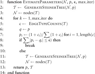
We apply an EM-like algorithm, presented as Algorithm 1, to identify the probability of each possible SD, CD and GD event. We initialize the method with uniform probability estimates, effectively leading to unweighted parsimony. Then, at each iteration of the algorithm, we infer a maximum likelihood directed Steiner tree (applying Algorithm 2) using the parameter values inferred at the previous iteration. We treat this as the E-step of the algorithm. This step is simplified relative to strict EM in that it uses a single optimal model fit, rather than an expectation over the solution space in the E-step as in our prior work (Pennington et al., 2007), but should yield comparable results to true EM in the limit of large numbers of tree edges. In the M-step, we then update the parameter values for each event based on the fraction of times that event is inferred across the tree edges, with the addition of a pseudocount of 1 (line 7) to account for events with inferred counts of zero.

2.2 Constructing a phylogenetic tree

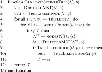
In Algorithm 1, the E-step involves generating phylogenetic trees via calls to a heuristic median-joining-based algorithm for inference of Steiner nodes in the tumor phylogenies. The key steps of this tree-building algorithm are summarized in Algorithm 2. The code first builds a directed minimum spanning tree (MST) $\mathcal{T}$ based on the observed cell types. As in standard median-joining (Bandelt et al., 1999), it uses a heuristic strategy to solve the hard problem of inferring unobserved Steiner nodes by seeking to identify triplets of taxa that can be more parsimoniously connected by positing an unobserved ‘median’ taxon sitting between them. Algorithm 2 iterates over each node triplet in $\mathcal{T}$ for which one node is the parent of the other two nodes in order to identify these median Steiner nodes that reduce tree cost. We define the lattice points of a triplet to be the set of configurations that agree in each dimension with at least one of the triplet. Each lattice point is considered in arbitrary order as a possible Steiner node. If a lattice point is not already in $\mathcal{T}$, a new tree, called the median tree, is created by adding that lattice point as a node and by connecting it via three edges with one incoming edge and two outgoing edges. If the resulting weight, calculated as explained in the following subsection, is less than the weight of the previous best tree, the lattice point is added to the tree. The best tree found by this procedure is returned.

Algorithm 1. Infer the rates of SD, CD and GD events using statistics from tumor phylogenies. The GenerateSteinerTree() routine uses Algorithm 2 to infer Steiner trees based on the set of cell states and parameter values. The vector p contains the current estimate of the probabilities of each mutation type, initialized with uniform rates in the present work. $\mathcal{N}$ represents the set of nodes in the most recently computed Steiner tree; initially, it is the set of configurations in the observed data. The positive value ϵ is a convergence tolerance, and $\text{max}\_\text{iter}$ is the maximum number of iterations. The algorithm returns an updated vector p of estimated mutation probabilities and final inferred phylogeny $\mathcal{T}$ on the input taxa $\mathcal{N}$ and any inferred Steiner taxa using the weights from the inferred p.

Algorithm 2. Main steps in the algorithm to generate tumor progression trees with particular rates for each of the SD, CD and GD events. $\mathcal{N}$ is a set of configurations that must be nodes of the generated tree. The vector p contains the probability of each type of mutation. The algorithm returns an inferred phylogeny $\mathcal{T}$ for the given inputs $\mathcal{N}$ and p.

2.3 Likelihood estimation

Although the basic median-joining strategy can be adapted to this application as a way of heuristically solving the hard problem of Steiner node inference, that strategy still depends on having a way to accurately estimate likelihoods and reconstruct likely paths of mutations between pairs of taxa. This latter task is very different for our model of copy number mutation than for more conventional character-based phylogenetics and requires novel theory and algorithms. The bulk of our theoretical conributions are directed to this sub-problem of finding minimum-weight paths between arbitrary pairs of taxa. We present here novel algorithms specifically for estimating the likelihood of the minimum weight SD + CD + GD path between two configurations. Due to space limitations, proofs of correctness of all of the claims in this section are deferred to Supplementary Materials.

In developing likelihood estimation algorithms, it is both conceptually and computationally easier to work with edge weights rather than edge probabilities. The weight w of an edge is related to the probability p of the event inferred across that edge by the formula w = −log p. Edge weights are additive, and the task of finding a maximum likelihood path or tree is equivalent to the task of finding a minimum weight path or tree.

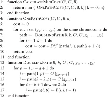
The process of finding minimum-weight SD + CD + GD paths is presented at a high level as Algorithm 3. The algorithm works in three steps. First, in the function DoublingPath, we calculate the shortest-length SD + GD path between configurations $C^s$ and $C^t$ for paths having $k=0,\dots ,m$ genome duplication events. Each of these paths defines a set of zero or more genome duplication points, configurations at which a genome duplication occurred. Second, in the function OnePathCost, we connect the endpoint of each genome duplication point with the start point of the next, or with $C^t$ for the last genome duplication, using minimum-weight SD + CD paths, computed using Algorithm 5. In the third and final step, at line 2, we choose the lowest-weight of these m + 1 SD + CD + GD paths; ties are irrelevant because we only need the path’s weight.

Algorithm 3. CalculateMinCost returns the minimum cost of converting a copy number profile $C^s(g_1,\dots ,g_d)$ to another copy number profile $C^t(g_1,\dots ,g_d)$ using combinations of SD, CD and GD events. $D_w^{s,ch}$ provides the minimum cost of an SD + CD path, as computed by Algorithm 5. $B$ is a table providing duplication points of minimum-weight SD + GD paths, derived by calling Algorithm 4.

2.4 Finding shortest-length SD + GD paths

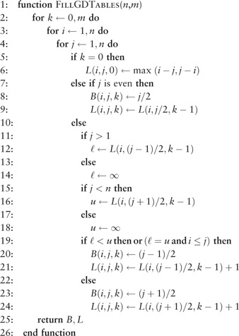
The function DoublingPath within Algorithm 3 is handled largely via a preprocessing step by which we construct a table of paths of mutation of single genes indexed by starting and ending copy numbers and numbers of whole-genome duplication events. This table is passed via the input B to Algorithm 3. For two configurations, and for a fixed number of genome duplication events, an SD + GD path with the minimum number of edges (i.e. the shortest-length path) may be quickly generated using this table. Pseudocode for this preprocessing step of finding optimal SD + GD paths is provided as Algorithm 4. For any fixed number of genome duplication events, the shortest-length SD + GD path between two configurations with the specified number of GD events may be computed one component at a time. For each component, a shortest length path may be found by adding SD losses or gains preceding and following genome duplication events to choose the most favorable duplication events given the starting and ending copy number. For a single component, shortest-length SD + GD paths have a well-defined structure. Briefly, for a fixed number of GD events, the condition that the SD + GD path be of minimal length requires that GD events be taken as late as possible. This observation is proved formally in Supplementary Theorem S17, provided in the Supplementary Material.

Given that the GD events in a SD + GD path must be taken as late as possible, there are only two possible ways a path containing a GD event may end: the path may end with a GD event (implying the end copy number is even) or the path may end in an GD event followed by an SD event (implying that the end copy number is odd). The observation suggests an algorithm for finding the duplication points in the shortest SD + GD path between copy numbers i and j for a single gene and a fixed number k genome duplications. One need only start at j, consider the one or two possible duplication points for the last GD event in a shortest-length SD + GD path terminating at j, and then choose the better of the duplication points by finding the shortest-length SD + GD path having exactly k − 1 duplications between $C^s$ and the duplication point. Algorithm 4 exploits this approach to construct a table of shortest paths for all pairs of taxa i and j, minimizing over the small set of possible numbers k of genome duplication events.

Consider the shortest SD + GD path between $(g_1,g_2)=(2,2)$ and (9, 6), with the condition that the path have exactly one genome duplication. One would first connect (2, 2) to (4, 3) with two gains of g₁ and one gain of g₂. Then one would insert an edge representing a genome duplication between (4, 3) and (8, 6). Finally, one would connect (8, 6) to (9, 6) using a single gain of g₁. Supplementary Theorem S17 implies that, for this example, inserting the one required genome duplication at any other copy number configuration would result in a path with more edges.

For a fixed number of genome duplication events, only a limited number of duplication points need to be considered. Moreover, because duplication increases copy number exponentially, it suffices to consider paths with $0,1,2,\dots ,m$ duplication events, where m = ⌈log₂(UB)⌉ (Supplementary Corollary S18 in Supplementary Materials). In our code, UB = 9, so m = 4.

In Algorithm 4, cases in which the copy number of some gene is zero in $C^s$ and $C^t$ are special. When a copy number starts at zero, there is no simple biological mechanism for daughter cells to regain that gene. Thus, we do not attempt to calculate paths for which a copy number changes from zero to non-zero, but rather just assign all such paths an infinite weight. Cases in which the copy number end at zero are also special. In such cases, the optimal SD + GD path is to lose all copies of the gene and then cycle from 0 to 0 on all genome duplication events. For brevity, we exclude such cases from the pseudocode, though code to handle these cases is implemented in the FISHtrees software.

2.5 Finding minimum-weight SD + CD paths

It remains to define an algorithm to identify a minimum-cost SD + CD path between two configurations, which we denote s and t. SD and CD steps may reordered so that the SD and CD steps that affect each chromosome are grouped together. For instance, if g₁ and g₂ are on chromosome 1, and g₃ and g₄ are on chromosome 2, one may generate an optimal path from $(2,2,2,2)$ to $(3,4,1,0)$ by taking an optimal SD + CD path from $(2,2,2,2)$ to $(3,4,2,2)$ in which each edge only affects genes on chromosome 1, and then following an SD + CD path from $(3,4,2,2)$ to $(3,4,1,0)$ in which each edge only affects genes on chromosome 2. Therefore, it suffices to consider the case in which all genes are on one chromosome.

Algorithm 4. Fill tables representing shortest length SD + GD paths for a single gene for all possible starting and ending copy numbers. $n$ represents the maximum copy number allowed for any gene and $m$ represents the maximum number of GD events to be considered. On exit, $B(i,j,k)$ contains the $k\text{th}$ duplication point and L(i, j, k) the number of SD gains and losses for the shortest length SD + GD path from $i$ to $j$, with the constraint that $k$ duplications occur.

The algorithm for computing the SD + CD distance is centered around the concept of a zigzag subpath, which is so named because its construction focuses on alternations between consecutive gain and loss events.

For example, consider the case of finding an optimal SD + CD path between $(g_1,g_2,g_3,g_4)=(2,2,2,2)$ and $(5,5,4,3)$, where all genes are on the same chromosome. Assuming equal edge weights, one may show that any optimal SD + CD path consists of three CD gains, one SD loss of g₃, and one SD gain each of g₁ and g₂. Whether such a path is of minimum weight is non-obvious and dependent on the weight of each type of edge. From theory developed in Supplementary Materials, it suffices to consider intermediate nodes on the zigzag path

$$\begin{array}{l}(2,2,2,2){\displaystyle \stackrel{CD}{\to }}(3,3,3,3){\displaystyle \stackrel{SD}{\to }}(3,3,3,2){\displaystyle \stackrel{CD}{\to }}(4,4,4,3)\\ {\displaystyle \stackrel{SD}{\to }}(4,4,3,3){\displaystyle \stackrel{SD}{\to }}(4,4,3,2){\displaystyle \stackrel{CD}{\to }}(5,5,4,3).\end{array}$$

This path demonstrates the characteristic pattern of gains and losses of a zigzag path: before each CD step, SD steps in the opposite direction are inserted to prevent the path from having an intermediate point with a more extreme copy number than the endpoint of the path. For the formal definition of a zigzag path, see Supplementary Materials.

A zigzag path as a whole may not be optimal, and in our example, is not optimal if all edges have equal weight. However, a key observation is that for endpoints s and t, there is an optimal SD + CD path that starts with a (possibly empty) subpath of a zigzag path ending at intermediate point r followed by a series of SD steps from r to t, but no further CD steps (Supplementary Theorem S13 of Supplementary Materials). Furthermore, the initial zigzag subpath, if non-empty, ends with a CD step. In our example of computing a path between (2, 2, 2, 2) and (5, 5, 4, 3), assuming that all edges have equal weights, the initial zigzag subpath ends at intermediate point (4,4,4,3). The remainder of the optimal path consists only of SD steps and may be trivially computed.

Between two configurations, there are two types of zigzag path, one containing only CD gains and the other containing only CD losses. It is shown in Supplementary Materials (Supplementary Lemma S3) that there is no advantage to considering SD + CD paths with gain and loss of the same chromosome. More surprisingly, it is shown that for a given chromosome, only one of the two zigzag paths may result in a beneficial series of zigzag steps and a non-zero cost (Supplementary Theorem S15). This mathematical result underlies the logic in Algorithm 5 that first tests if taking the CD gain zigzag path leads to a benefit. If so, this sense is used to find a provably optimal SD + CD path, otherwise the CD loss zigzag path is used. The pseudocode is presented as Algorithm 5, which defines a variable σ (for sense) that takes the value − 1 to indicate a zigzag loss (a zigzag subpath having only CD losses) or 1 to indicate a zigzag gain.

Algorithm 5. Compute the weight of an optimal SD + CD path between configurations s and t, assuming all genes are on the same chromosome. The vectors w⁺ and w⁻ contain the weights of SD gains and losses, respectively, and ${\gamma }^{+}$ and ${\gamma }^{-}$ are the weights of CD gains and losses. The algorithm returns the cost of a minimum-weight path between s and t for the input weight function, assuming only SD and CD events are used.

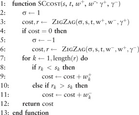Thus, we need to define a subroutine to determine the cost of an initial, possibly zero-length, beneficial zigzag path and its endpoint. The algorithm is based on Supplementary Theorem S13 of Supplementary Materials and pseudocode is presented as Algorithm 6. After each CD step of sense σ is added to the zigzag path, the algorithm tests whether adding the CD step, and the SD steps of the opposite sense that precede it, has lower cost than terminating the initial zigzag subpath after the previous CD step, or at the start if there is no previous CD step. The endpoint of the best initial subpath and the cost of this subpath are returned. At lines 8–9, the costs of the SD steps that undo some of the effects of the CD step are tallied. At lines 10–11, the benefits of using a CD step to change the counts of multiple genes in one step are tallied. If benefits exceed costs, then at lines 14–15, the count is changed by 1 for those genes that are modified by the CD step but do not have a compensatory SD step of the opposite sense.

2.6 Complexity analysis

We conclude the description of methods by analyzing the complexity of our algorithms. For this analysis, we denote the maximum number of GD events as m, the upper bound of gene copy number (UB) as n, the total number of probes as d, and the total number of unique copy number profiles (taxa) in a dataset as l. We separately parameterize by the number of Steiner nodes introduced, s, because while this could in principle be as large as ${(n+1)}^d$ it is in practice a small constant.

Algorithm 6. Compute an optimal initial zigzag path of sense σ from s on the way to t, assuming all genes are on the same chromosome. The vector a represents the weight of SD steps of sense σ, b representing the cost of SD steps of the opposite sense, and γ is the cost of a CD step of sense σ. The algorithm returns the cost of the inferred path, full cost, and the ending taxon r of the initial zigzag path, which will itself be an intermediate node on the path from s to t.

We are primarily interested in the running time of Algorithm 1, for which the time per iteration is dominated by the cost of calling Algorithm 2, which in turn is dominated by the cost of the algorithm used to find directed MSTs. The MST algorithm finds an optimal tree with $\ell$ nodes, out of a dense graph of $\mathcal{O}({\ell }^2)$ possible edges. The implementation in FISHtrees uses the method of Karp (1971), which has a complexity of $\mathcal{O}({\ell }^3)$. The complexity can be reduced to $\mathcal{O}({\ell }^2)$ using the method of Tarjan (1977).

The number of calls to the MST routine in Algorithm 2 is bounded by the number of triplets considered, $\mathcal{O}(l^3)$, and the number of possible lattice points examined per triplet, $\mathcal{O}(3^d)$. Because only the lattice points from triplets involving the observed taxa are considered, the number of Steiner nodes added does not affect the number of calls to the MST routine. It does, however, affect the complexity of finding an optimal MST, yielding a worse-case bound of $\mathcal{O}\left({(\ell +s)}^3\right)$ operations. Thus, in total, the calls to the MST routine in Algorithm 2 have complexity $\mathcal{O}\left({\ell }^3{(\ell +s)}^3{3}^d\right)$.

In addition, each application of the MST algorithm requires us to generate pairwise distances through $\mathcal{O}({(l+s)}^2)$ calls to Algorithm 3. The cost of these calls does not approach the cost of applying the MST algorithm, in theory or practice. It can be shown that an application of Algorithm 3, including the calls to Algorithms 5 and 6 requires $\mathcal{O}(m^{2}n{d}^2)$ operations, which may also be understood as $\mathcal{O}(d^2)$ as m and n are parameters that are rarely changed. Algorithm 4 is irrelevant to the complexity analysis as it produces a table that does not depend on the observed data and that for typical values of m and n comfortably fits in memory on a typical desktop computer in 2015. Accumulating all of these contributions gives us a total running time of $\mathcal{O}(l^3{(l+s)}^3{3}^d+{(l+s)}^2(m^{2}n{d}^2))$ for Algorithm 2 and for each iteration of Algorithm 1.

Typical values of the parameters in practice for current FISH datasets are $n\approx 9,m\approx \lfloor {\log }_{2}n\rfloor \approx 3,d\approx 8$, and $l\approx 250$. Theoretical running times are polynomial in all factors except d. Because actual times on datasets of this approximate size are measured in seconds (see ‘Simulation Results’ in Supplementary Materials S2) the method can be expected to remain practical for appreciably larger numbers of cells (l) as might be anticipated for newer FISH data. Significantly larger numbers of probes (larger d) would be problematic for the present algorithms, however, and alternatives might thus be needed if single-cell sequencing becomes practical for estimating copy numbers of large numbers of cells. It is difficult to judge how numbers of iterations of Algorithm 1 required for convergence might be affected by much larger l or d, leaving some uncertainty about performance on data characteristics one might reasonably anticipate in the future, although the number of iterations needed is effectively a small constant for the datasets currently available to us.

3 Results

We applied our parameter inference algorithms to FISH datasets on two kinds of human cancers: cervical cancer and oral (tongue) cancer. The primary datasets used are as follows: (i) Dataset CC1 (Wangsa et al., 2009) consists of paired primary and metastatic cervical cancer samples collected from 16 patients and primary samples collected from 15 patients whose tumors did not metastasize probed on four oncogenes residing on distinct chromosomes (LAMP3, PROX1, PRKAA1 and CCND1); (ii) Dataset TC [D.Wangsa et al., submitted] consists of 65 single samples collected from tongue cancer patients probed for four genes located on distinct chromosomes (TERC, EGFR, CCND1, TP53), with tumor stages [ranging from 1 (least advanced) up to four (most advanced)] available on all patients and tobacco usage (a known risk factor), survival, and disease-free survival out to 73 months available on most patients. Because neither of these datasets have more than one probe per chromosome, we do not consider CD events in these tests. Two additional datasets, both of which have multiple genes on at least one chromosome, are analyzed in the Supplementary Materials.

We have additionally conducted a series of simulation tests to verify that the method accurately infers phylogenies and model parameters from data of known ground truth. These tests verify on a set of five parameter scenarios that the methods are effective at inferring accurate model parameters in the presence of a range of mutation rates between genes, chromosomes, and whole-genome events. The tests further confirm that the resulting phylogeny inferences are substantially more accurate than those derived from standard phylogeny algorithms applied to the same data across the range of scenarios and that this accuracy is achieved with realistic sizes of dataset. Due to space limitations, these simulation results are deferred to the Supplementary Material. The protocol for generating simulated data is described under Simulation Methods in the section Supplementary Methods. The results appear under Simulation Results in the section Supplementary Results and in Supplementary Figures S4–S9.

3.1 Identifying progression markers in cervical cancer (CC1) data

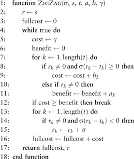
We applied our algorithm on each of the samples in each of the datasets separately and inferred probabilities of each SD and GD event. We show the boxplots for the inferred parameter values in the CC1 dataset in Figure 1, across 31 primary (Fig. 1A) and 16 metastatic (Fig. 1B) samples. ‘Gain of LAMP3’ is the most frequent event in both primary and metastatic samples, similar to the findings reported in our past work (Chowdhury et al., 2013).

Fig. 1.

Inferred probabilities of events for primary (A) and metastatic (B) cervical samples. WGD refers to the rate of whole-genome duplications

Next, for each pair of 16 primary and 16 metastatic samples, we performed statistical tests based on the ‘tree edge count’ statistic, which quantifies, for each tumor phylogenetic tree, the total number of edges across which gain or loss of each gene is inferred. Because the four genes analyzed in the CC1 dataset are all oncogenes, we focused on gains, although losses do occur sometimes. To investigate further whether each of the four genes may be more important in the primary or metastatic phase of cervical cancer, we computed the proportion of edges that represent gains of that gene in each sample for the 16 pairs. We present results for PROX1 with some motivation from previous studies of this gene. A prior study of colorectal cancer showed by various experimental techniques that overexpression of PROX1 is a driver of a pre-cancerous dysplasia leading to the primary tumor (Petrova et al., 2008). This study led others to investigate the hypothesis that overexpression or copy number gains of PROX1 would be similarly important in primary cervical cancers. However, static analysis of these CC1 FISH data (Wangsa et al., 2009) and an unrelated dataset in which PROX1 protein expression was measured by immunohistochemisty (Sotiropoulou et al., 2010) gave no significant results about PROX1.

Using our models, a paired t-test of the proportion of tree edges that are PROX1 gains showed a significantly higher proportion in the primary tumors (P-value < 0.007, one-sided, nominal; P-value < 0.028, corrected for multiple testing of four genes). The unpaired t-test also gave nominal significance (P-value < 0.042, one-sided). A less powerful unpaired Wilcoxon test of the proportions (P-value < 0.04, one-sided) and an even less powerful binomial test comparing which of the two proportions is greater in each pair (P-value < 0.04, one-sided) both supported the conclusion that the proportion of edges that are PROX1 gains is greater in the primary CC1 samples. These results are consistent with the colorectal cancer study (Petrova et al., 2008) and show how dynamic modeling of tumor progression can give insights that static analysis misses.

3.2 Classification of cervical samples

We performed classification experiments using tree-based features to separate samples from different stages of cervical cancer in CC1. We used these experiments to validate our models and demonstrate their value, based on our past observation that tree progression models allow one to distinguish between trees drawn from distinct current or future progression states (Chowdhury et al., 2013, 2014). We used the following set of tree-based features: (i) edge count: eight features corresponding to the fractions of progression tree edges showing gains and losses of each gene; (ii) Tree level: features corresponding to the fraction of cells at each depth in the progression trees; (iii) Parameter values: nine features corresponding to inferred gain and loss probability of each gene (SD), and the probability of a whole genome duplication event (GD).

We applied these methods for three classification tasks: (a) distinguishing primary samples that progressed to metastasis from their paired metastatic samples, (b) distinguishing all primary samples from all metastatic samples and (c) distinguishing primary samples that metastasized from primary samples that did not metastasize. We compared the classification performance of the features from our current model with the SD-only (pure rectilinear) model (Chowdhury et al., 2013) and unweighted SD + GD (Chowdhury et al., 2014) model of tumor progression. Because each gene resides on a distinct chromosome in CC1, CD events are irrelevant. We performed 500 rounds of bootstrapping and computed mean accuracy and standard deviations of accuracy.

The results are presented in Figure 2. The parameter value-based features (i.e. the inferred phylogenetic rate models themselves) are the most accurate predictors for the first and second tasks of separating primary samples from the metastatic ones. For the clinically important problem of determining whether a given primary tumor will metastasize, tree level features show improved prediction accuracy by at least 3.5% over all other feature sets considered, including comparable feature sets from the earlier unweighted models.

Fig. 2.

Classification results on the CC1 dataset

3.3 Survival analysis in the TC dataset

For the TC dataset, we focused our analyses of the tree-progression models on trying to identify predictors of survival. Based on earlier work suggesting that the distribution of node depth was a useful predictor of progression in CC1 (Chowdhury et al., 2013), we investigated whether the tree level cell distribution is also a predictor of overall and disease-free survival time in TC. Similarly to the cervical cancer samples, we considered distribution of cells across all the levels of the tumor phylogenetic trees inferred on the tongue cancer samples. Using the cell distribution vector as features, we performed K-means clustering to partition the samples into two subgroups. We used ‘Euclidean’ as the distance measure for the clustering and performed clustering with 10 restarts using the new initial cluster centroid position.

We performed Kaplan–Meier (KM) analysis (survdiff function in R) to compare either the survival time or the disease-free survival time between the two groups obtained from the two subgroups of samples (Fig. 3). The subgrouping of patients yielded a significant difference in overall (P-value = 0.0443, two-sided) and disease-free (P-value = 0.0371, two-sided) survival between the two patient groups. The good prognosis cluster was assigned 33 patients and the bad prognosis cluster was assigned 32 patients. Some insight into the differences in the two groups can be gained by examining the cluster centers. The cluster center of the good prognosis group has 33% of its weight in the first 5 tree levels and 90% of its weight in the first 10 tree levels, while the cluster center of the bad prognosis group has only 16% of its weight in the first 5 tree levels and only 51% of its weight in the first 10 tree levels. We repeated the same clustering procedure and KM analyses using trees derived from our previous unweighted SD + GD algorithm (Chowdhury et al., 2014) but did not observe statistically significant differences in overall (P-value = 0.0784) or disease-free (P-value = 0.14) survival between the two patient groups with the older methods.

Fig. 3.

KM curves for the test of association between overall (A) and disease-free (B) survival time and tree level cell count statistics-based subgrouping of patients

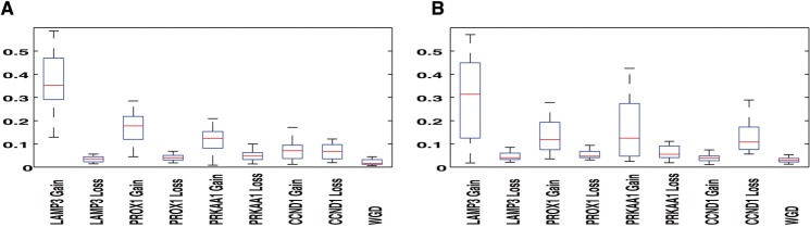
We then performed multivariate survival analysis using the Cox proportional hazards (COXPH) model (survfit function in R) to test whether the new test statistics can predict survival or disease-free survival independent of tumor stage. The results are presented in Figure 4. The combined P-value is statistically significant, showing that the two covariates are independently associated with overall (disease-free) survival time. The hazard ratio is higher to a significant degree for tree statistic-based subgrouping compared to tumor stage, meaning there is a higher risk of death (disease) if a patient is assigned to the higher risk category by the tree statistic subgrouping, independent of tumor stage.

Fig. 4.

COXPH analysis to test the correlation between tree level cell count statistic-based subgrouping of patients and tumor stage with disease-free and overall survival time

4 Discussion

We have developed algorithms for the problem of inferring tumor-specific mutation parameters and applying these to improve single-tumor phylogenetic tree inference at the cellular level, with specific application to inferring multiscale copy number evolution from single-cell FISH data. This work involved developing efficient algorithms for a weighted parsimony model of copy number evolution, which required substantially different methods than the unweighted model in (Chowdhury et al., 2014). We then used an EM-like inference method to learn weight parameters jointly with tree building, providing for the first time scalable algorithms capable of learning tree models for hundreds to thousands of single cells isolated from individual tumors. This work addresses a key need for learning tumor-specific evolutionary models capable of dealing with realistic levels of cellular heterogeneity in single tumors. We showed that the resulting models provide insight into tumor-specific variation and lead to improved prediction of future tumor progression in multiple tumor types.

This work makes an important step towards scalable algorithms for inferring cancer-specific evolution in single tumors, although much remains to be done to realize the full potential of the approach. There are many possible avenues for improvement in the methods, either to more closely approach true optima for the given objective function or to develop novel objectives describing more realistic and detailed models of tumor evolution mechanisms without sacrificing efficiency. Alternative approaches for inferring evolutionary models from the phylogenies, such as the phylogenetic profiling approaches of Csűrös (2010), may also provide more accurate and detailed parameter inferences for any given objective function and phylogeny inference algorithm. Another important limitation is the focus on FISH data. FISH is currently the only technology for which it is practical to profile genomic variation in hundreds of single cells per patient for moderate-sized patient populations, an essential feature for tumor progression prediction. The present work thus focused on models of copy number evolution specifically, as it is both the most common form of hypermutability in tumor evolution (Heng et al., 2013) and the mechanism most easily profiled by FISH. FISH, however, offers a far more limited portrait of variation of each cell than does single-cell sequencing (Navin et al., 2011). Although single-cell sequencing is not yet practical for the numbers of cells needed to study variation in evolutionary mechanisms across patient populations, one can reasonably anticipate that it will eventually overcome that limit, motivating new algorithmic problems to deal simultaneously with hundreds to thousands of cells, potentially millions of markers of variation, and with the diverse classes of genomic variation that sequencing data can reveal.

Funding

This research was supported in part by the Intramural Research Program of the U.S. National Institutes of Health, National Cancer Institute, and National Library of Medicine, and by U.S. National Institutes of Health grants 1R01CA140214 (R.S. and S.A.C.) and 1R01AI076318 (R.S.).

Conflict of Interest: none declared

References

- Bandelt H., et al. (1999) Median-joining networks for inferring intraspecific phylogenies. Mol. Biol. Evol., 16, 37–48. [DOI] [PubMed] [Google Scholar]
- Beaumont M.A. (2010) Approximate Bayesian computation in evolution and ecology. Annu. Rev. Ecol. Evol. Syst., 41, 379–406. [Google Scholar]
- Beerenwinkel N., et al. (2015) Cancer evolution: mathematical models and computational inference. Syst. Biol., 64, e1–e25. [DOI] [PMC free article] [PubMed] [Google Scholar]
- Chowdhury S.A., et al. (2013) Phylogenetic analysis of multiprobe fluorescence in situ hybridization data from tumor cell populations. Bioinformatics, 29, i189–i198. [DOI] [PMC free article] [PubMed] [Google Scholar]
- Chowdhury S.A., et al. (2014) Algorithms to model single gene, single chromosome, and whole genome copy number changes jointly in tumor phylogenetics. PLoS Comp. Biol., 10, e1003740. [DOI] [PMC free article] [PubMed] [Google Scholar]
- Csűrös M. (2010) Count: evolutionary analysis of phylogenetic profiles with parsimony and likelihood. Bioinformatics, 26, 1910–1912. [DOI] [PubMed] [Google Scholar]
- Dempster A.P., et al. (1977) Maximum likelihood from incomplete data via the EM algorithm. J. R. Stat. Soc. B, 39, 1–38. [Google Scholar]
- Desper R., et al. (1999) Inferring tree models of oncogenesis from comparative genomic hybridization data. J. Comput. Biol., 6, 37–51. [DOI] [PubMed] [Google Scholar]
- Desper R., et al. (2000) Distance-based reconstruction of tree models for oncogenesis. J. Comput. Biol., 7, 789–803. [DOI] [PubMed] [Google Scholar]
- Di Noia J., Neuberger M. (2007) Molecular mechanisms of antibody somatic hypermutation. Annu. Rev. Biochem., 76, 1–22. [DOI] [PubMed] [Google Scholar]
- Felsenstein J. (2004) Inferring Phylogenies . Sinauer Associates, Inc., Sunderland, MA. [Google Scholar]
- Fisher R., et al. (2013) Cancer heterogeneity: implications for targeted therapeutics. Br. J. Cancer , 108, 479–485. [DOI] [PMC free article] [PubMed] [Google Scholar]
- Greenman C.D., et al. (2010) Estimation of rearrangement phylogeny for cancer genomes. Genome Res., 22, 346–361. [DOI] [PMC free article] [PubMed] [Google Scholar]
- Greenblatt M.S., et al. (1994) Mutations in the p53 tumor suppressor gene: clues to cancer etiology and molecular pathogenesis. Cancer Res., 54, 4855–4878. [PubMed] [Google Scholar]
- Harris R., et al. (2002) RNA editing enzyme APOBEC1 and some of its homologs can act as DNA mutators. Mol. Cell , 10, 1247–1253. [DOI] [PubMed] [Google Scholar]
- Heng H.H., et al. (2013) Chromosome instability (CIN): what it is and why it is crucial to cancer evolution. Cancer Metastasis Rev., 32, 325–340. [DOI] [PubMed] [Google Scholar]
- Heselmeyer-Haddad K., et al. (2012) Single-cell genetic analysis of ductal carcinoma in situ and invasive breast cancer reveals enormous tumor heterogeneity, yet conserved genomic imbalances and gain of MYC during progression. Am. J. Pathol., 181, 1807–1822. [DOI] [PMC free article] [PubMed] [Google Scholar]
- Hjelm M., et al. (2006) New probabilistic network models and algorithms for oncogenesis. J. Comput. Biol., 13, 853–865. [DOI] [PubMed] [Google Scholar]
- Karp R.M. (1971) A simple derivation of edmonds’ algorithm for optimum branchings. Networks, 1, 265–272. [Google Scholar]
- Liu J., et al. (2009) Inferring progression models for CGH data. Bioinformatics, 25, 2208–2215. [DOI] [PubMed] [Google Scholar]
- Loeb L.A. (1991) Mutator phenotype may be required for multistage carcinogenesis. Cancer Res., 51, 3075–3079. [PubMed] [Google Scholar]
- Martins F.C., et al. (2012) Evolutionary pathways in BRCA1-associated breast tumors. Cancer Discov., 2, 503–511. [DOI] [PMC free article] [PubMed] [Google Scholar]
- Marusyk A., Polyak K. (2010) Tumor heterogeneity: causes and consequences. Biochim. Biophys. Acta (BBA) Rev. Cancer, 1805, 105–117. [DOI] [PMC free article] [PubMed] [Google Scholar]
- Navin N., et al. (2011) Tumour evolution inferred by single-cell sequencing. Nature, 472, 90–94. [DOI] [PMC free article] [PubMed] [Google Scholar]
- Newton M.A. (2002) Discovering combinations of genomic aberrations associated with cancer. J. Am. Stat. Assoc., 97, 931–942. [Google Scholar]
- Nowell P.C. (1976) The clonal evolution of tumor cell populations. Science, 194, 23–28. [DOI] [PubMed] [Google Scholar]
- Pennington G., et al. (2007) Reconstructing tumor phylogenies from heterogeneous single-cell data. J. Bioinform. Comput. Biol., 5, 407–427. [DOI] [PubMed] [Google Scholar]
- Petrova T.V., et al. (2008) Transcription factor PROX1 induces colon cancer progression by promoting the transition from benign to highly dysplastic phenotype. Cancer Cell, 13, 407–419. [DOI] [PubMed] [Google Scholar]
- Purdom E., et al. (2013) Methods and challenges in timing chromosomal abnormalities within cancer samples. Bioinformatics, 29, 3113–3120. [DOI] [PMC free article] [PubMed] [Google Scholar]
- Snuderl M., et al. (2011) Mosaic amplification of multiple receptor tyrosine kinase genes in glioblastoma. Cancer Cell, 20, 810–817. [DOI] [PubMed] [Google Scholar]
- Sotiropoulou N., et al. (2010) Tumour expression of lymphangiogenic growth factors but not lymphatic density is implicated in human cervical progression. Pathology, 42, 629–636. [DOI] [PubMed] [Google Scholar]
- Sprouffske K., et al. (2011) Accurate reconstruction of the temporal order of mutations in neoplastic progression. Cancer Prev. Res., 4, 1135–1144. [DOI] [PMC free article] [PubMed] [Google Scholar]
- Szerlip N.J., et al. (2012) Intratumoral heterogeneity of receptor tyrosine kinases EGFR and PDGFRA amplification in glioblastoma defines subpopulations with distinct growth factor response. Proc. Natl Acad. Sci. U.S.A., 109, 3041–3046. [DOI] [PMC free article] [PubMed] [Google Scholar]
- Tarjan R.E. (1977) Finding optimum branchings. Networks, 7, 25–35. [Google Scholar]
- Timmermann B., et al. (2010) Somatic mutation profiles of MSI and MSS colorectal cancer identified by whole exome next generation sequencing and bioinformatics analysis. PLoS One, 5, e15661. [DOI] [PMC free article] [PubMed] [Google Scholar]
- Urbschat S., et al. (2011) Clonal cytogenetic progression within intratumorally heterogeneous meningiomas predicts tumor recurrence. Int. J. Oncol., 39, 1601–1608. [DOI] [PubMed] [Google Scholar]
- Wang Y., et al. (2014) Clonal evolution in breast cancer revealed by single nucleus genome sequencing. Nature, 512, 155–160. [DOI] [PMC free article] [PubMed] [Google Scholar]
- Wangsa D., et al. (2009) Fluorescence in situ hybridization markers for prediction of cervical lymph node metastases. Am. J. Pathol., 175, 2637–2645. [DOI] [PMC free article] [PubMed] [Google Scholar]
Associated Data
This section collects any data citations, data availability statements, or supplementary materials included in this article.