Detection of urinary bladder mass in CT urography with SPAN

Abstract

Purpose:

The authors are developing a computer-aided detection system for bladder cancer on CT urography (CTU). In this study, the authors focused on developing a system for detecting masses fully or partially within the contrast-enhanced (C) region of the bladder.

Methods:

With IRB approval, a data set of 70 patients with biopsy-proven bladder lesions fully or partially immersed within the contrast-enhanced region (C region) of the bladder was collected for this study: 35 patients for the training set (39 malignant, 7 benign lesions) and 35 patients for the test set (49 malignant, 4 benign lesions). The bladder in the CTU images was automatically segmented using the authors’ conjoint level set analysis and segmentation system, which they developed specifically to segment the bladder. A closed contour of the C region of the bladder was generated by maximum intensity projection using the property that the dependently layering contrast material in the bladder will be filled consistently to the same level along all CTU slices due to gravity. Potential lesion candidates within the C region contour were found using the authors’ Straightened Periphery ANalysis (SPAN) method. SPAN transforms a bladder wall to a straightened thickness profile, marks suspicious pixels on the profile, and clusters them into regions of interest to identify potential lesion candidates. The candidate regions were automatically segmented using the authors’ autoinitialized cascaded level set segmentation method. Twenty-three morphological features were automatically extracted from the segmented lesions. The training set was used to determine the best subset of these features using simplex optimization with the leave-one-out case method. A linear discriminant classifier was designed for the classification of bladder lesions and false positives. The detection performance was evaluated on the independent test set by free-response receiver operating characteristic analysis.

Results:

At the prescreening step, the authors’ system achieved 84.4% sensitivity with an average of 4.3 false positives per case (FPs/case) for the training set, and 84.9% sensitivity with 5.4 FPs/case for the test set. After linear discriminant analysis (LDA) classification with the selected features, the FP rate improved to 2.5 FPs/case for the training set, and 4.3 FPs/case for the test set without missing additional true lesions. By varying the threshold for the LDA scores, at 2.5 FPs/case, the sensitivities were 84.4% and 81.1% for the training and test sets, respectively. At 1.7 FPs/case, the sensitivities decreased to 77.8% and 75.5%, respectively.

Conclusions:

The results demonstrate the feasibility of the authors’ method for detection of bladder lesions fully or partially immersed in the contrast-enhanced region of CTU.

1. INTRODUCTION

Bladder cancer is the fourth most common cancer diagnosed in men, with 1 in 26 men developing bladder cancer during their life. The American Cancer Society estimates that during 2014, around 15 580 deaths (11 170 men and 4410 women) will occur due to bladder cancer, and about 74 690 new cases (56 390 in men and 18 300 in women) will be diagnosed in the United States.¹ Early detection and treatment of bladder cancer increase patient survivability. If the bladder cancers are detected and treated while the cancer is confined within the bladder’s inner lining and has not invaded the muscular bladder wall, the 5-yr survival rate is 88%, but drops to 63% if the cancer is detected after it has invaded the bladder wall but is still confined to the bladder; however, only about half of the patients are diagnosed before the cancer has invaded the muscular bladder wall.¹

Multidetector row CT urography (CTU) has become the imaging modality of choice for most urinary track abnormalities. CTU, as a single exam, can be used to evaluate the kidneys, intrarenal collecting systems, and ureters and therefore may spare the patients from having to undergo other imaging studies, resulting in reduced health care costs.^2–6

Interpretation of a CTU study requires thorough image analysis, often requiring extensive time. On average, 300 slices are generated for each CTU scan at a slice interval of either 1.25 mm or 0.625 mm (range: 200–600 slices). The radiologist interpreting the study must visually determine the presence of lesions within the urinary tracts on a display workstation, frequently adjusting the brightness, contrast, and zoom levels. The radiologist must pay close attention throughout the entire urinary tract as multiple lesions may be present. In addition, many different urinary anomalies may be found in a single CTU study. Not only do the radiologists have to identify these anomalies but also they must determine their likelihood of being an urothelial neoplasm. The challenges of analyzing a CTU study lead to a substantial variability among radiologists in detection of bladder cancer, with reported sensitivities ranging from 59% to 92%.^7,8 The chance that the radiologist misses a subtle lesion may not be negligible due to the workload of analyzing CTU studies; thus, any technique that may help radiologists identify urothelial neoplasms will be useful. Computer-aided detection (CAD), used as an adjunct, may reduce the chance of oversight by the radiologists. We are developing a CAD system that detects bladder cancer in CTU to be used for such purposes.

Few investigators have worked on CAD for bladder cancer to-date. Duan et al.⁹ used an adaptive window setting to segment bladder tumor surfaces for magnetic resonance (MR) cystography. They generated multiple windows that covered the inner wall of the bladder and from which features were extracted. Using quadratic discriminant analysis, they determined if a window contained a true positive or false positive in a data set of ten patients. Jaume et al.¹⁰ detected bladder tumors in abdominal CT images by estimating the bladder wall thickness using inner and outer bladder surface meshes generated using the marching cubes algorithm. They separated each of the 26 bladders in their data set into six regions and created an atlas to distinguish between normal and diseased regions. Hadjiiski et al.¹¹ performed a pilot study in detecting lesions within the contrast-enhanced region of the bladder in 15 patients in CTU. They used a rule-based system based on shape measures and uniformity measures to identify lesion candidates.

Automatic detection of bladder lesions in CTU is challenging. The imaged bladders, along with their lesions, can assume a variety of shapes and sizes. Bladders may also be partially or fully filled with intravenous (IV) contrast material that opacifies a portion of the bladder. The lesions in the bladder region that is filled with contrast material have much different contrasts relative to the surroundings than those in the bladder region that is not filled with contrast material. This requires different strategies for the detection of lesions in the contrast-enhanced (C) and noncontrast (NC) regions of the bladder.

In this study, we focused on developing a system for detection of bladder lesions fully or partially immersed in the C region of the bladder. We designed the system and evaluated its performance using free-response receiver operating characteristic (FROC) analysis using a data set of 70 cases. Although the data set was still small, to our knowledge it was the largest data set compared to that used in other reported studies.

2. MATERIALS AND METHODS

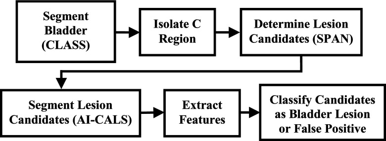
The bladder within the CTU images was automatically segmented within a manually marked bounding box; then, as part of the prescreening step, the C region was delineated from the segmented bladders. The bladder wall of the C region was transformed into a wall thickness profile that was analyzed to determine lesion candidates. These candidates were automatically segmented, and morphological features were extracted. The best subset of these features was determined and a linear discriminant classifier was designed with a training set for classification of the bladder lesions and false positives. The block diagram of the detection system is presented in Fig. 1. The detection performance was evaluated in an independent test set by FROC analysis.

FIG. 1.

Block diagram of the detection system.

2.A. Data set

With approval of the Institutional Review Board, a data set of 70 patients undergoing CTU who subsequently underwent cystoscopy and biopsy was collected retrospectively from the Department of Radiology at the University of Michigan. The CTU scans were acquired with GE Healthcare LightSpeed MDCT scanners at a slice interval of 1.25 mm or 0.625 mm using 120 kVp and 160–560 mAs and reconstructed with filtered back projection using the standard reconstruction kernel. The excretory phase images used were obtained 12 min after the initiation of the first bolus of a split-bolus intravenous contrast injection and 2 min after the initiation of the second bolus of 175 ml of nonionic contrast material at a concentration of 300 mg iodine/ml. Since patients were not turned prior to image acquisition, dependently layering IV contrast material that had been excreted into the renal collecting systems partially or fully filled the bladder on the CTU images.

All lesions were marked by experienced radiologists in the CTU volumes as reference standard. Two radiologists (26 years of experience and 16 years of experience) marked the lesion by placing a ROI over the lesion, indicating the starting and ending slices of the lesion, measuring the longest diameter of the lesion, and giving a subtlety rating. Consensus was obtained if the lesion locations were different, and the final call was correlated with radiology and pathology reports and biopsy results. The size and subtlety of the lesions given by the single, more experienced radiologist were reported to illustrate the detection performance of the system for lesions of different degrees of difficulty as seen by an experienced radiologist.

A total of 99 biopsy-proven bladder lesions were identified in the fully or partially contrast-enhanced region of the bladder. The cases were split evenly into independent training and test sets. The training set contained 35 subjects having 38 malignant and 7 benign lesions with an average size of 20.1 mm (range: 4.2–61.7 mm), measured as the longest diameter on an axial slice [Fig. 2(a)]. The test set contained 35 subjects having 49 malignant and 4 benign lesions with an average size of 18.8 mm (range: 1.4–61.1 mm) [Fig. 2(a)]. The average lesion subtlety ratings in both sets were 2.2 (scale 1–5, 5 very subtle) [Fig. 2(b)].

FIG. 2.

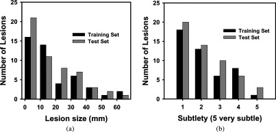
Histograms of lesion size (a) and lesion subtlety (b) for lesions in the training and test set. The average lesion size was 20.1 mm (range: 4.2–61.7 mm) for the training set, and 18.8 mm (range: 1.4–61.1 mm) for the test set. The average lesion subtlety ratings in both sets were 2.2 (scale 1–5, 5 very subtle).

For image processing purposes, all CT voxel values in terms of Hounsfield units (HU) are linearly shifted into gray level, where gray level  =  HU + 1024 so that all image voxel values are positive.

2.B. Bladder segmentation using conjoint level set analysis and segmentation system (CLASS)

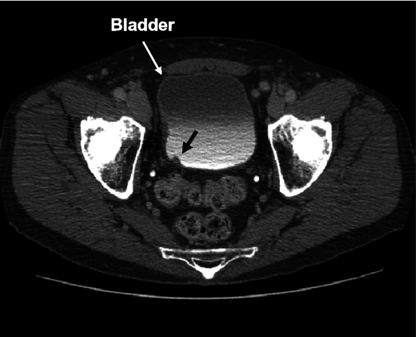
A critical component of CAD system that detects bladder cancer is accurate bladder segmentation that isolates the bladder from the surrounding anatomical structures. An axial CTU scan of the bladder is shown in Fig. 3. The bladder shown is partially filled with IV contrast material and a malignant lesion can be identified in the lower, contrast-enhanced portion of the bladder. The presence of the two distinct regions that have very different attenuation values, a region filled with IV contrast material and a region without contrast material, poses a challenge for segmentation algorithm that needs to go across the strong boundary.

FIG. 3.

An axial slice of a CTU scan in which the bladder is partially filled with IV contrast material. A malignant lesion is present in the contrast-enhanced region of the bladder, indicated by the bold arrow.

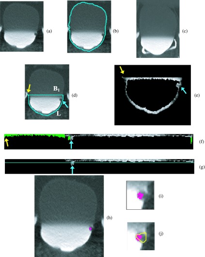
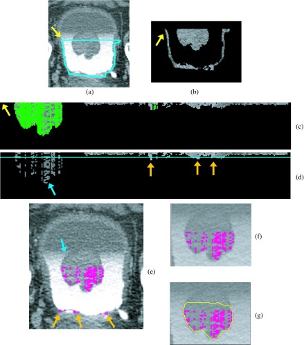
We are developing a software package, referred to as the CLASS, for segmenting the bladder in CTU. We introduced CLASS previously.^12,13 CLASS consists of four stages: (1) preprocessing and initial segmentation, (2) 3D level set segmentation, (3) 2D level set segmentation, and (4) local contour refinement. CLASS segments the noncontrast and the contrast-enhanced regions of the bladder by applying the level sets to each region separately, refining the contours, and then automatically conjoins them. The CLASS segmentation is initialized by two manually placed approximate bounding boxes (ROIs) for the contrast and noncontrast regions of the bladder. The boxes were generated by a single researcher who was trained by the radiologists and has been involved in the development of the system for 2 yr. More details of the bladder segmentation methods can be found in the literature.^12,13 An example of a bladder and its segmentation are shown in Figs. 4(a) and 4(b), respectively.

FIG. 4.

Bladder lesion candidate prescreening and segmentation—example of true positive. (a) ROI of the CTU slice that includes the lesion. (b) Bladder segmentation of the slice encompassing the bladder wall. (c) MIP of the bladder used to determine the boundary between the contrast-enhanced and noncontrast regions. (d) Segmentation of the contrast-enhanced region of the bladder (L contour). The horizontal line on top of the contour is the boundary between the NC and C regions of the bladder, B₁. The arrow on the left side of the bladder indicates the starting point for the wall thickness profile. The arrow on the right points to a true lesion. (e) Magnified C region image after adaptive thresholding. (f) Bladder wall profile. Highlighted pixels were removed during the false positive reduction of voxel candidate. The left section of the profile was removed using location-based rules as described in Sec. 2.C.3. (g) Bladder wall profile used for candidate detection. The line is the threshold used to determine lesion candidates. The arrow points to a lesion candidate, which is mapped onto the bladder in (h). (i) Magnified image of the region around the lesion candidate. The windowing of the image was adjusted to better visualize the bladder wall. (j) Lesion candidate segmentation. The segmentation refines the highlighted initial region, resulting in a better representation of the lesion.

2.C. Bladder wall profile generation and lesion candidate identification with Straightened Periphery ANalysis (SPAN)

Bladder lesion candidates are identified by first isolating the contrast-enhanced region of the bladder, and then by using our newly developed method, referred to as SPAN. SPAN consists of three stages: (1) wall thickness profile generation, (2) false positive reduction of voxel candidate, and (3) lesion candidate identification.

2.C.1. Isolating the contrast-enhanced region of the bladder

The contrast-enhanced region of the bladder is separated from the noncontrast region using the property that the dependently layering IV contrast material in the bladder will be filled to the same level consistently along all CTU slices due to gravity. We use maximum intensity projection (MIP) along the slices of the bladder to estimate the upper boundary of the contrast-enhanced region. The ROIs initializing the segmentation of the C and NC regions of the bladder are used to determine the range of the CTU slices for the MIP. As the bladder is located on top of the pelvic bones when the patient lies in a supine position, it is common that the bones intrude into the bladder’s ROI toward the bottom of the bladder. If the bright bones show up on the MIP image, its interference makes it difficult to accurately determine the upper level of the contrast material. Therefore, only a portion of the slices included in the ROI is used. We experimentally determined that 30% of the slices toward the bottom of the bladder from the best slice (to avoid the pelvic bones) and 90% of the slices toward the top of the bladder from the best slice (to avoid other organs above the bladder) worked the best. The best slice is the slice that best represents the bladder region, e.g., where the bladder is seen the largest. It was selected manually when the ROIs were defined. A MIP image is shown in Fig. 4(c).

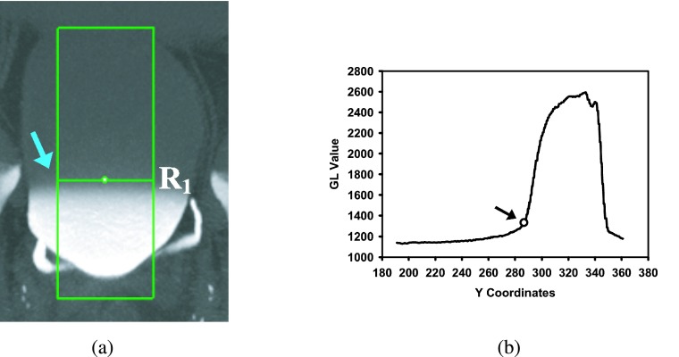
From the MIP image, a gray level profile is generated as described below. The two ROI boxes marked for the NC and C region segmentations are combined to create a rectangular box such that the width of the box is the width of intersection of the NC and C boxes and the height is the union of the heights of the NC and C boxes. Then, the box’s width is reduced by 50% while keeping the same center [Fig. 5(a)] to minimize the negative effects of the peripheries of the irregularly shaped bladders on the estimation of the transition point between the contrast and noncontrast regions. For every row of the box, the gray levels of the pixels belonging to the row are averaged and recorded into a profile [Fig. 5(b)]. The profile is analyzed to find the first row R₁ whose average gray level is greater than a gray level threshold Th_p. By using the training data set, the Th_p was determined experimentally as 1330 which provided adequate separation of the NC and C regions for the training cases. A horizontal line B₁ at row R₁ that intersects with the bladder boundary is determined as the boundary between the NC and C regions of the bladder [Fig. 4(d)]. The portion of the C region of the bladder contour and the B₁ boundary then form a new closed contour, referred to as the L contour, that encloses the C region [Fig. 4(d)]. The image pixels that are within the L contour, i.e., the C region of the bladder, are analyzed in the subsequent steps.

FIG. 5.

Estimation of boundary (row R₁) between the NC and C regions. (a) The box used to calculate the average bladder GL profile shown in (b). The arrow points to the row of which the y-coordinate was determined to be that of R₁. (b) Profile of the average GL values for each row of the box in (a). The arrow indicates the average GL of the first row that has value above the 1330 threshold and therefore identified as R₁.

2.C.2. Wall thickness profile generation with SPAN

Generating the bladder wall thickness profile using the previously obtained C region image and L contour involves two steps: (1) adaptive thresholding of the contrast material and (2) transformation of the L contour to a straightened wall profile.

2.C.2.a. Adaptive thresholding.

The contrast material within the C region is removed by adaptive thresholding. Using a constant threshold for the contrast material may result in missing lesions that have relatively high gray levels in some cases and may also lead to portions of the contrast material not being eliminated that may become false positives in other cases. Using adaptive thresholding method resolves these potential issues.

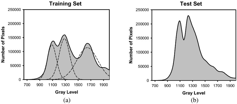
For each slice within the C region, the mean and the standard deviation of the pixel gray levels are calculated. For pixels whose gray level was greater than 1800, their gray level was set to 1800 for calculating the average. The average gray level, GL_Avg, is stratified into four different groups which are used to determine the initial threshold, Th_init, using the following decision rules:

$${\displaystyle {\text{Th}}_{\text{init}}=\left\{\begin{array}{cc}\hfill {\text{Th}}_I^H\hfill & \hfill {\text{GL}}_{\text{Avg}}\ge {\text{Th}}_I^H\hfill \\ \hfill {\text{Th}}_I^{\text{MH}}\hfill & \hfill {\text{Th}}_I^{\text{MH}}\le {\text{GL}}_{\text{Avg}}<{\text{Th}}_I^H\hfill \\ \hfill {\text{Th}}_I^{\text{ML}}\hfill & \hfill {\text{Th}}_I^{\text{ML}}\le {\text{GL}}_{\text{Avg}}<{\text{Th}}_I^{\text{MH}}\hfill \\ \hfill {\text{Th}}_I^L\hfill & \hfill {\text{GL}}_{\text{Avg}}<T{h}_I^{\text{ML}}\hfill \end{array}\right.,}$$ (1)

where ${\text{Th}}_I^H$, ${\text{Th}}_I^{\text{MH}}$, ${\text{Th}}_I^{\text{ML}}$, and ${\text{Th}}_I^L$ are the high, medium high, medium low, and low gray level thresholds, respectively. The thresholds were determined after analyzing the histogram of pixel gray levels within the C region using the training set. The histograms of pixel gray levels within the C region for both the training and test sets are shown in Fig. 6. Assuming a Gaussian mixture distribution, multiple Gaussians were fit to the histogram for the training set [Fig. 6(a)], and the peaks of the Gaussians (${\text{Th}}_I^{\text{MH}}$, ${\text{Th}}_I^L$) along with intersections of the Gaussians that corresponded to a sharp drop in the histogram (${\text{Th}}_I^H$, ${\text{Th}}_I^{\mathrm{ML}}$) were used as the thresholds after adjusting for outlier cases (Table I). The peak of the Gaussian whose gray level was above 1330 was not used as a threshold, as our analysis during the isolation of the C region showed that these pixels are generally part of the contrast material and not the bladder wall. For slices with high GL_Avg, Th_init is set to be ${\text{Th}}_I^H$ to ensure most of the contrast material is removed after thresholding. For slices with average contrast enhancement between ${\text{Th}}_I^H$ and ${\text{Th}}_I^{\text{MH}}$, setting Th_init to be ${\text{Th}}_I^{\text{MH}}$ will remove the majority of the contrast material in the slice (Table I and Fig. 6). Th_init is set to be ${\text{Th}}_I^{\text{ML}}$ for slices with GL_Avg within the range of ${\text{Th}}_I^{\text{MH}}$ to ${\text{Th}}_I^{\text{ML}}$ which are usually near the end of the bladder. The amount of contrast material in these slices is generally less than the amount in slices near the center of the bladder, resulting in lower intensity of the contrast region. The slices whose GL_Avg is less than ${\text{Th}}_I^{\text{ML}}$ typically are those with C regions that were not well-enhanced by the contrast material. These slices require a smaller gray level threshold or the contrast material would not be removed; thus, their Th_init is set to be ${\text{Th}}_I^L$.

FIG. 6.

Histogram of gray level values of pixels within the C region of the (a) training set and (b) test set. The multiple Gaussians that were fitted to the training set to determine threshold values are shown with dotted lines in (a).

TABLE I.

Parameter values for adaptive thresholding in wall thickness profile generation.

${\text{Th}}_I^H$	${\text{Th}}_I^{\text{MH}}$	${\text{Th}}_I^{\text{ML}}$	${\text{Th}}_I^L$	ε	λ	τ	${\text{Th}}_{\text{GL}}^H$	${\text{Th}}_{\text{GL}}^L$
1400	1300	1200	1150	15	−60	20	100	80

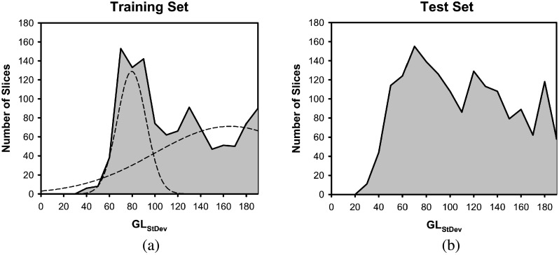
The gray level threshold for the contrast material, Th_C, is then refined adaptively by both Th_init and the standard deviation of the pixel gray levels, GL_StDev, within the C region as follows:

$${\displaystyle {\mathrm{Th}}_C=\left\{\begin{array}{cc}\hfill {\mathrm{Th}}_{\mathrm{init}}-\frac{{\mathrm{GL}}_{\mathrm{StDev}}}{\epsilon }\hfill & \hfill {\mathrm{GL}}_{\mathrm{StDev}}\ge {\mathrm{Th}}_{\mathrm{GL}}^H\hfill \\ \hfill {\mathrm{Th}}_{\mathrm{init}}-\lambda \hfill & \hfill {\mathrm{Th}}_{\mathrm{GL}}^L\le {\mathrm{GL}}_{\mathrm{StDev}}<{\mathrm{Th}}_{\mathrm{GL}}^H\hfill \\ \hfill {\mathrm{Th}}_{\mathrm{init}}+\tau \hfill & \hfill {\mathrm{GL}}_{\mathrm{StDev}}<{\mathrm{Th}}_{\mathrm{GL}}^L\hfill \end{array}\right.,}$$ (2)

where ε, λ, and τ are constants, and ${\mathrm{Th}}_{\mathrm{GL}}^H$ and ${\mathrm{Th}}_{\mathrm{GL}}^L$ are the high and low thresholds for GL_StDev, respectively. Using the training set, the constants were determined experimentally, while the thresholds were determined by analyzing the histogram of the GL_StDev. The histogram of GL_StDev for both the training and test set is shown in Fig. 7. After fitting two Gaussians to the histogram of the training set GL_StDev [Fig. 7(a)], the peak of one of the Gaussians, ${\mathrm{Th}}_{\mathrm{GL}}^L$, and the intersection of the Gaussians corresponding to a sharp drop, ${\mathrm{Th}}_{\mathrm{GL}}^H$, on the histogram were used as the thresholds, leading to three different categories. For slices with GL_StDev greater than ${\mathrm{Th}}_{\mathrm{GL}}^H$, the C region is usually very inhomogeneous and requires a lower threshold to ensure most of the contrast material is removed. For slices with GL_StDev values in the range of ${\mathrm{Th}}_{\mathrm{GL}}^L$ to $h_{\mathrm{GL}}^H$, they generally also contain pixels with high gray levels so that the Th_init is also lowered to ensure that sufficient contrast material is removed for the subsequent stages. Slices with GL_StDev values lower than ${\mathrm{Th}}_{\mathrm{GL}}^L$ usually contain fairly homogeneous C region. The dependent layering of the contrast material on these slices is not as prevalent as other slices with higher GL_StDev; thus, their gray level is lower. These cases need a higher threshold to ensure that lesions are not removed along with the contrast material. The values of the chosen constants and thresholds are shown in Table I.

FIG. 7.

Histogram of standard deviation values of pixel gray level within the C region of a CTU slice, GL_StDev for the (a) training set and (b) test set. The multiple Gaussians that were fitted to the training set to determine threshold values are shown with dotted lines in (a).

Once Th_C is determined, the contrast material is eliminated from within the C region by setting the gray level to 0 for all pixels whose gray level is greater than Th_C. Examples of C region images after adaptive thresholding are shown in Figs. 4(e), 8(b), and 9(b). Comparison of the C region with and without the adaptive thresholding for cases in the three different GL_StDev categories is shown in Fig. 10. Notice that without the adaptive thresholding [Figs. 10(d)–10(f)], much of the contrast material remains within the C region image, which would lead to incorrect wall thickness profiles and thus missing lesion candidates and false positive detections. With adaptive thresholding, well-defined bladder wall can be obtained [Figs. 10(g)–10(i)].

FIG. 8.

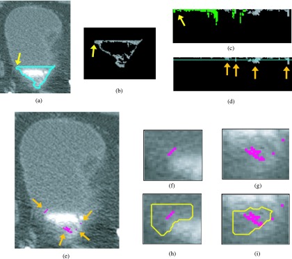
Bladder lesion candidate prescreening and segmentation at a slice near the end of the bladder—example of false positives. (a) Segmentation of the C region of the bladder (L contour). (b) C region image after adaptive thresholding. (c) Bladder wall profile. Highlighted pixels were removed during the false positive reduction of voxel candidate. (d) Bladder wall profile used for candidate detection. The line is the threshold used to determine lesion candidates. The arrows point to lesion candidates. (e) Lesion candidates projected onto the bladder. Arrows point to lesion candidates. [(f) and (g)] Magnified image of the region around the lesion candidate. [(h) and (i)] Lesion candidate segmentation. Two single pixel lesion candidates shown in (e) and (g) were discarded during the lesion candidate determining stage using the size criteria. The two remaining candidates were both false positive lesions and were removed by the LDA classifier.

FIG. 9.

Bladder lesion candidate prescreening and segmentation for a lesion along B₁—example of true positive. (a) Segmentation of the C region of the bladder (L contour). (b) C region image after adaptive thresholding. (c) Bladder wall profile. Highlighted pixels were removed during the false positive reduction of voxel candidate. (d) Bladder wall profile used for candidate detection. The line is the threshold used to determine lesion candidates. The arrows point to lesion candidates. (e) Lesion candidates projected onto the bladder. Arrows point to lesion candidates. (f) Magnified image of the region around the lesion candidate. The windowing of the image was adjusted to better visualize the lesion. (g) Lesion candidate segmentation. The three candidate pixel regions at the bottom of the bladder were discarded during the lesion candidate determining stage using the size criteria.

FIG. 10.

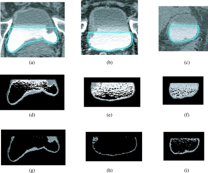
C region images with and without adaptive thresholding for cases that fall within the different categories of GL_StDev. [(a)–(c)] Bladder slices with L contour with different standard deviations, GL_StDev: (a) GL_StDev = 133, (b) GL_StDev = 89, and (c) GL_StDev = 77. [(d)–(f)] C region after hard thresholding slices in (a)–(c) using Th_C of 1330 without adaptive thresholding. [(g)–(i)] C region after adaptive thresholding with rules in Eq. (3) for slices in [(a)–(c)]. (g) Th_C = 1191, (${\mathrm{GL}}_{\mathrm{StDev}}\ge {\mathrm{Th}}_{\mathrm{GL}}^H$), (h) Th_C = 1140, (${\mathrm{Th}}_{\mathrm{GL}}^L\le {\mathrm{GL}}_{\mathrm{StDev}}<{\mathrm{Th}}_{\mathrm{GL}}^H$), (i) Th_C = 1220, (${\mathrm{GL}}_{\mathrm{StDev}}<{\mathrm{Th}}_{\mathrm{GL}}^L$).

2.C.2.b. Wall profile generation.

Once the contrast material is removed from the slice, a straightened profile of wall thickness is generated by mapping all of the points along the L contour, L_i, i = 1,  …,  n, sequentially to the X-axis of a new coordinate system such that L_i(x_i, y_i) has the coordinate (X_i,0). The origin of this new coordinate system is defined at the top left of the profile, with Y-values increasing in the downward direction. For a given pixel L_i(x_i, y_i), the path normal to the point toward the interior of the L contour is calculated using the normal angle θ defined as

$${\displaystyle \theta =90°+\frac{1}{2}\left({tan}^{-1}\left(\frac{y_i-y_{i-1}}{x_i-x_{i-1}}\right)+{tan}^{-1}\left(\frac{y_{i+1}-y_i}{x_{i+1}-x_i}\right)\right),}$$ (3)

where (x_i+1, y_i+1) and (x_i−1, y_i−1), respectively, are the coordinates of the next L_i+1 and previous L_i−1 neighboring points of L_i. The pixels along the normal path are sequentially mapped onto the profile at increasing Y-values such that the new coordinates of the pixels are given by (X_i, Y_j) j = 1,  …,  i_m, while X_i is fixed. The path along the normal ends when four black pixels are encountered consecutively, indicating that the path reaches the lumen of the C-region where the pixel gray level has been set to 0. The number of pixels along the normal path at L_i is denoted by i_m. Figures 4(f), 8(c), and 9(c) show examples of the transformation. Pixels that will be removed by the following false reduction step are also marked in the figures.

2.C.3. False positive reduction of voxel candidate with SPAN

False positive reduction is applied to the straightened bladder wall profile. One step for reducing false positives is to remove pixels with gray level values above 1100 on the profile in the section corresponding to B₁ of the L contour. Columns on the profile in the section whose starting points, (X_i,0), have a gray level value above 1100 are also removed. Because the B₁ section is the border separating the C region and the NC region of the bladder, the gray level of the region along B₁ is often lower than other regions within the C region of the bladder. This may cause many false positive findings, as the darker regions transformed onto the profile may be marked as lesion candidates. After studying lesions in the training set that are located near B₁, we found that the pixels of lesions within the B₁ region typically have gray level values less than 1100. By applying this criterion, we can reduce false positive findings that may be caused by the lower pixel gray levels of the profile along the B₁ boundary neighboring the noncontrast region.

Sharp peaks along the bladder wall profile that are likely caused by noise are also removed. Since noise is random and forms small peaks, we set a criterion to exclude peaks less than three pixels in width and greater than five pixels in height relative to its surroundings. Examples of SPAN for a true lesion, false positive lesions, and a lesion located along B₁ are shown in Figs. 4(f), 8(c), and 9(c), respectively.

2.C.4. Lesion candidate identification with SPAN

Lesion candidates are found by analyzing the bladder wall profile. For a given bladder profile, the average height of the profile (μ) is calculated, excluding the pixels from the B₁ section (the border between the NC and C regions) and locations whose height is greater than 10 pixels. The standard deviation (σ) of the pixels used is also calculated, and a height threshold (H), in pixels, is set using the following equation, which was determined experimentally to maximize the number of true positives found while keeping the false positive findings low:

$${\displaystyle H=\mathrm{floor}\left(\mu -\frac{\sigma }{2}+0.8\right)+2,}$$ (4)

where the floor function represents the rounding down operation. On the profile, pixels with heights larger than H are considered to be lesion candidate pixels [Figs. 4(g), 8(d), and 9(d)]. After the lesion candidate pixels are identified, they are mapped back to the original bladder slices as lesion candidate voxels [Figs. 4(h), 4(i), 8(e)–8(g), 9(e) and 9(f)].

The lesion candidate voxels are then grouped into regions. Candidate voxels that are one slice apart, and within five voxels apart in 3D space, are clustered into the same region. A candidate voxel is ignored if there are no other candidate voxels that are within five voxels on the same slice. Regions that contain less than five candidate voxels or greater than 50 000 candidate voxels are ignored. This size range was determined by analyzing the training cases. Each of the regions retained is enclosed with a 3D bounding box to indicate a ROI for a lesion candidate.

2.D. Lesion candidate segmentation, feature extraction, and classification

2.D.1. Lesion segmentation with autoinitialized cascaded level set (AI-CALS)

Using the ROI obtained for a lesion candidate, the lesion is segmented from the surrounding tissue using the AI-CALS segmentation system.¹⁴ The AI-CALS system consists of three stages: preprocessing, initial segmentation, and level set segmentation. While this process seems similar to the CLASS system used for bladder segmentation, AI-CALS uses a different method for initial segmentation, and different sets of parameters, which were specifically developed for segmentation of bladder lesions. In the first stage, preprocessing techniques are applied in 3D to the ROI obtained from the candidate prescreening process above. Smoothing, anisotropic diffusion, gradient filters, and the rank transform of the gradient magnitude are applied to the slices within the ROI to obtain a set of smoothed images, a set of gradient magnitude images, and a set of gradient vector images. The set of smoothed images is used in the second stage, while the other two sets are used during level set propagation in the third stage.

We modified the AI-CALS method in the second stage to improve the lesion segmentation performance for this study. In the second stage, the system automatically labels a subset of voxels in the ROI for analysis based on the attenuation, gradient, and location of the voxels. First, voxels with gray level value below 600 are removed. The voxels with gradient values in the top 50% of all voxels in the ROI are identified using the gradient magnitude image and removed from the ROI. In order to distinguish between the contrast material and the lesion candidate that may be present within the ROI, a step that uses Otsu’s method is added, which is not part of the original AI-CALS. The region with voxel gray level values between 1024 and the threshold gray level determined by the Otsu’s method is marked by a binary mask. An elliptical cylinder whose radius is 0.8 of the width and height of the ROI, centered at the centroid of the binary mask, is placed within the binary mask. The intersection of the binary mask and the elliptical cylinder is labeled as the object region. In the original AI-CALS, an ellipsoid centered at the ROI is to determine the object region; however, we found that using an ellipsoid causes the lesions to be undersegmented toward the first and last slices of the ROI, while using an elliptical cylinder, as described above, alleviates this problem. A morphological dilation filter with a spherical structuring element of 2 voxels in radius, 3D flood fill algorithm, and a morphological erosion filter with a spherical structuring element of 2 voxels in radius is applied to the object region to connect neighboring components and extract an initial segmentation surface.

In the third stage, the initial segmentation surface is propagated toward the lesion boundary using cascading level sets. Our chosen level set implementation evolves according to the following equation:

$${\displaystyle \frac{\partial }{\partial t}\mathrm{\Psi }\left(x\right)=-\alpha A\left(x\right)\cdot \nabla \mathrm{\Psi }\left(x\right)-\beta P\left(x\right)\left|\nabla \mathrm{\Psi }\left(x\right)\right|+\gamma \kappa \left(x\right)\left|\nabla \mathrm{\Psi }\left(x\right)\right|,}$$ (5)

where α, β, and γ are the coefficients for the advection, propagation, and curvature terms, respectively; A(x) is a vector field image (assigning a vector to each voxel in the image) which drives the contour to move toward regions of high gradient; P(x) is a scalar speed term between 0 and 1 causing the contour to expand at the local rate; and $\kappa \left(x\right)=\mathrm{div}\left(\nabla \mathrm{\Psi }\left(x\right)/\left|\nabla \mathrm{\Psi }\left(x\right)\right|\right)$ is the mean curvature of the level set at point x. The symbol ∇ denotes the gradient operator and div is the divergence operator.¹⁵

Three 3D level sets with predefined sets of parameters are applied in series to the initial segmentation surface. The corresponding parameters of the three level sets are presented in Table II.

TABLE II.

Parameters for the AI-CALS level sets.

Level set	α	β	γ	n
First	1	2	1	10
Second	1	0.4	q	100
Third	0	1.0	0	20
2D slices	4.0	0.3	0.5	100

The first 3D level set slightly expands and smoothes the initial contour. The second 3D level set not only brings the contour toward the sharp edges but also expands it slightly in regions of low gradient. The parameter “q” in Table II is defined to be a linear function σM + ϕ of the 2D diagonal distance M of the ROI box in millimeters (mm), where σ  =  0.06, ϕ = − 0.11 as shown previously.¹⁵ The third 3D level set further draws the contour toward sharp edges. As a final step, a 2D level set is applied to every slice of the segmented object to refine the 3D contours using the 3D level set contours as the initial contour. Further details on the AI-CALS method can be found in the literature.¹⁴ Examples of true and false segmented bladder lesion candidates are shown in Figs. 4(j), 8(h), 8(i), and 9(g).

2.D.2. Feature extraction and classification

For each segmented lesion candidate, 23 morphological features are automatically extracted from the central slice of the segmented lesion. Five of the morphological features are based on the normalized radial length, which is defined as the Euclidean distance from the object’s centroid to each of its edge pixels, i.e., the radial length, normalized relative to the maximum radial length of the object.¹⁶ Table III lists the features that were used. The definitions of these features can be found in the literature.¹⁷ These features are studied because we found that these features are useful for lesion classification from our previous experience with breast masses.

TABLE III.

Table of morphological features used.

NRL	Shape-based	Gray level-based
NRL mean	Perimeter	Ten contrast features
NRL standard deviation	Area	Gray level average
NRL entropy	Circularity	Gray level standard deviation
NRL area ratio	Rectangularity
NRL zero crossing count	Perimeter-to-area ratio
	Fourier descriptor

Using the training set, stepwise feature selection is used to select the best feature subset. Using simplex optimization with leave-one-out case method, the best combination of values for the feature selection parameters, F_in, F_out, and tolerance, is determined from the training set. Features for classification are then selected from the entire training set with the best thresholds. The six features selected were normalized radial length area, rectangularity, area, average gray level, and two contrast features. More details about these features and the feature selection can be found in the literature.¹⁸ A linear discriminant analysis (LDA) classifier was then designed with the training set for classification of the bladder lesions and false positives using the selected features as input predictor variables. The trained LDA classifier was applied to the test set for independent testing.

2.E. Evaluation methods

The performance of the lesion candidate prescreening steps was evaluated by determining the sensitivity and specificity. The overall performance of the bladder lesion detection CAD system with feature extraction and FP reduction by the LDA classifier was evaluated using FROC analysis using our in-house developed package that calculated the sensitivity and specificity at specific operating points. The FROC curve was generated by varying the decision threshold for the LDA discriminant scores.

3. RESULTS

At the prescreening step, our system achieved 84.4% (38/45) sensitivity with an average of 4.3 false positives per case (FPs/case) for the training set, and 84.9% (45/53) sensitivity with 5.4 FPs/case for the test set. The prescreening step generated 215 lesion candidates for the training set, (66 true lesion candidates and 149 false positive lesion candidates), which were used to train the LDA classifier.

Tables IV and V summarize the detected lesions during prescreening by size and subtlety, respectively. For both the training and test sets, most of the lesions that were missed had subtlety ratings of greater than 3 and were smaller than 10 mm; however, the detection system was able to find the majority of the lesions that fit into these categories. For lesions smaller than 10 mm, 66.7% (10/15) and 71.4% (15/21) were found by the system in the training and test sets, respectively (Table IV). For lesions with subtlety ratings greater than 3, 60.0% (9/15) of them were detected in the training set, while 78.9% (15/19) of them were detected in the test set (Table V). The system detected 86.8% (33/38) and 85.7% (42/49) of the malignant lesions in the training and test sets.

TABLE IV.

Detected lesions at the prescreening stage for lesions of different sizes.

	Lesion size (mm)
	0–10	10–20	20–30	30–40	40–50	50–60	60–70
Training set	66.7% (10/15)	100% (14/14)	50.0% (2/4)	100% (6/6)	100% (3/3)	100% (1/1)	100% (2/2)
Test set	71.4% (15/21)	100% (11/11)	85.7% (7/8)	85.7% (6/7)	100% (3/3)	100% (2/2)	100% (1/1)

TABLE V.

Detected lesions at the prescreening stage for lesions of different subtleties.

	Lesion subtlety (1–5, 5 very subtle)
	1	2	3	4	5
Training set	100% (18/18)	84.6% (11/13)	100% (5/5)	50.0% (4/8)	0% (0/1)
Test set	90.0% (18/20)	85.7% (12/14)	90.0% (9/10)	83.3% (5/6)	33.3% (1/3)

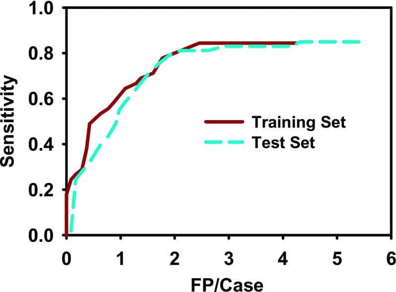
Using feature extraction and LDA classifier, the false positive (FP) rate improved to 2.5 FPs/case for the training set and 4.3 FPs/case for the test set without missing additional true lesions. By varying the threshold for the LDA scores, the FROC curve was generated as shown in Fig. 11. At 2.5 FPs/case, the training set achieved a sensitivity of 84.4%, while the test set achieved 81.1%. At 1.7 FPs/case, the sensitivities were 77.8% and 75.5% for the training and test sets, respectively. Table VI shows the sensitivities of the system at different false positive rates for the training and test sets.

FIG. 11.

FROC curves for automatic computer detection after feature classification with LDA. After prescreening, the system achieved 84.4% sensitivity with 4.3 FPs/case for the training set, and 84.9% sensitivity with 5.4 FPs/case for the test set. After LDA classification, at 1.7 FPs/case, the sensitivities were 77.8% and 75.5% for the training and test sets, respectively.

TABLE VI.

Sensitivity at a given FP rate after using LDA classifier.

	False positive rate (FPs/case)
	0.5	1.0	1.5	2.0	2.5	3.0
Training set (%)	48.9	64.4	70.0	77.8	84.4	84.4
Test set (%)	36.6	54.7	70.6	80.0	81.1	83.0

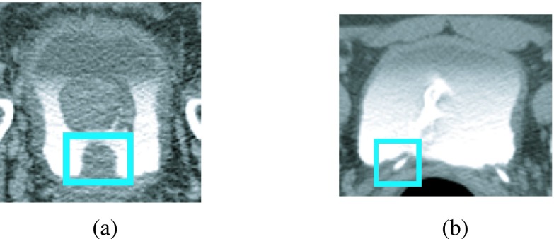
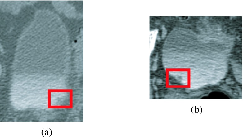
Examples of true positive lesions detected are shown in Fig. 12. Figure 13 shows examples of false positive detections, while Fig. 14 shows lesions that were missed.

FIG. 12.

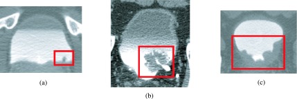
Examples of detected bladder lesion. Lesions of varying sizes and shapes were correctly identified by the CAD system. (a) Small lesion located at the bottom of the bladder. (b) Large lesion partially obstructing the ureterovesical junction. (c) Lesion covering large amount of the bladder wall. All three lesions were malignant.

FIG. 13.

Examples of false positives. (a) Prostate protruding onto the bladder was detected as a lesion candidate. (b) Ureterovesical junction detected as a lesion candidate. Neither was removed by the LDA classifier.

FIG. 14.

Examples of lesions missed by prescreening. The inhomogeneous contrast material in both (a) and (b) prevented the prescreening steps from identifying these lesion candidates. Both were malignant lesions.

4. DISCUSSION

In this study, we developed a system that can automatically detect bladder lesions of a wide range of sizes and subtleties within the contrast-enhanced region of the bladders in CTU that only requires two ROI boxes as inputs. At the preprocessing stage, the system detected over 80% of the lesions in both the training and test sets, while having about 5 FPs/case.

Our system was able to detect lesions of various shapes and sizes at different locations within the contrast-enhanced region of the bladder. Small lesions protruding out from the bladder wall, large lesions that occupy a large portion of the contrast-enhanced region, and bladder masses that look like an extension of the bladder wall were all detected by the system (Fig. 12).

During the prescreening stage, a relative large number of false positive lesions appeared close to the ends of the bladder. This may be caused by the fact that the CT slices at these locations are close to or even intersect the bladder wall in some regions; the partial volume effects may contribute to the inhomogeneous and low contrast appearance of the bladder region [Fig. 7(e)]. However, the LDA classifier was able to correctly remove the two false positives shown in that example. A common false positive finding that the LDA classifier has difficulty to differentiate from true lesions is the prostate in male patients. For some cases, the prostate protruding into the bladder has a similar appearance as a lesion [Fig. 13(a)]. The bladder segmentation may also leak into the prostate due to the interface between the bladder and the prostate being difficult to distinguish. The detection system, therefore, identifies the portions of the prostate that are segmented as lesion candidates. Another common cause of false positive findings not removed by the LDA classifier is the ureterovesical junction (UVJ). When the location near the UVJ is imaged, the ureter wall at the junction between the ureter and the bladder may appear as a protrusion from the bladder wall, similar to a lesion [Fig. 13(b)], which the system detects as a lesion candidate. A common cause for false negatives is the nonuniformity of the contrast material that camouflages the lesions as a part of the bladder wall (Fig. 14).

Our system detected the majority of both the malignant and the benign lesions. For both the training and the test sets, more malignant lesions were detected than benign lesions. However, the number of benign lesions was much smaller than the number of malignant lesions in our data set. Therefore, we cannot draw a conclusion on whether the system detection performance is related to lesion malignancy.

With feature extraction and FP reduction by LDA, our system achieved 84.4% sensitivity with an average of 2.5 FPs/case for the training set, and 84.9% sensitivity with 4.3 FPs/case for the test set. Our radiologist and urologist coinvestigators expect that a CAD system with 85%–90% sensitivity with 2 FPs/case for the entire bladder would be useful in their practice. We were close to reaching this goal for our training set, but the system needs to be improved to meet our performance goals for unknown cases.

Our system takes approximately 2–5 min to run for a case on a system with an Intel Xeon 5160 processor at 3 GHz, depending on the bladder size. It takes approximately 2 min/case for manual input, which includes loading the case and marking the two ROIs.

We have performed a sensitivity analysis of our CAD system by changing the ROI box size, ROI centroid, and best slice locations. The size of the ROI box was changed in the range from −5% up to 20% in the X–Y direction. The centroid of the ROI box was randomly shifted by 5% in the X or Y direction. The best slice of the ROI box was randomly moved by −5% or 5%. The sensitivity of each ROI box change was estimated at the operating points used for the original box for the training (2.5 FPs/case) and test (4.3 FPs/case) sets and shown in Tables VII and VIII. Overall, we observed stable performance for lesion detection within the ranges of ROI box sizes and locations studied.

TABLE VII.

Detection sensitivity at 2.5 FPs/case for training set.

ROI change	Original	XY − 5%	XY + 5%	XY + 10%	XY + 15%	XY + 20%	Best slice ± 5%	XY centroid ± 5%
Sensitivity (%)	84.4	77.8	82.2	82.2	86.7	86.7	82.2	84.4

TABLE VIII.

Detection sensitivity at 4.3 FPs/case for test set.

ROI change	Original	XY − 5%	XY + 5%	XY + 10%	XY + 15%	XY + 20%	Best slice ± 5%	XY centroid ± 5%
Sensitivity (%)	84.9	84.9	83.0	81.1	84.9	73.6	86.8	84.9

It is difficult to make a direct comparison with the previous methods by other investigators described in the Introduction due to the differences in the data sets, lesion sizes and subtlety, and the performance evaluation methods. In the study by Jaume et al.,¹⁰ they delineated each bladder in their data set into six different zones and measured the performance by determining whether or not a zone was diseased or not. Duan et al.⁹ measured their performance by determining the percentage in which the lesions in their data set were covered by windows marking a region representing a part of a lesion. In comparison to our pilot study,¹¹ in which 83% of bladder lesions were detected with 1.4 FPs/case using a data set of 15 cases, the current system had sensitivities of 84.4% and 84.9% at a FP rate of 2.5 and 4.3 FPs/case for the training and test sets, respectively. When the system from our pilot study was applied to the larger data set used in this study, it had sensitivities of 77.8% and 50.9% at a FP rate of 2.6 and 2.7 FPs/case for the training and test sets, respectively. Our current system achieved a higher sensitivity when using a data set of 70 patients compared to the system in our pilot study.

This study has several limitations. First, the detection method was designed for detection in the contrast-enhanced region of the bladder. As the contrast between the lesion and its surroundings is much smaller in the noncontrast region, a different method will have to be developed for detection in the noncontrast region. Second, this study was directed toward detection of bladder masses, but not bladder wall thickenings. Wall thickening that was found by the system was not considered to be a true lesion and excluded as a false positive in this study. A different method may need to be developed to detect wall thickenings accurately, as wall thickenings possess different characteristics than masses. We will develop methods to detect bladder lesions in the noncontrast region and bladder wall thickenings in future studies as components of a complete CAD system for detection of bladder cancer.

5. CONCLUSION

This study demonstrates the feasibility of our method for detection of bladder lesions located fully or partially in the contrast-enhanced region of the CTU scans for lesions of a variety of shapes and sizes. The prescreening stage detected most of the true lesions, but also many false positive lesions. Using feature extraction and a trained classifier, the false positives were reduced while keeping the sensitivity high. The results indicate the usefulness of the methods for bladder lesion detection for lesions partially or fully within the contrast-enhanced region of CTU. Further work is underway to increase the sensitivity, detect lesions within the noncontrast-enhanced region, and detect lesions manifested as bladder wall thickening. This study is a step toward the development of a CAD system for detection of urothelial lesions imaged with CT urography.

REFERENCES

- 1.American Cancer Society, “What are the key statistics about bladder cancer?,” www.cancer.org (2014).
- 2.Akbar S. A., Mortele K. J., Baeyens K., Kekelidze M., and Silverman S. G., “Multidetector CT urography: Techniques, clinical applications, and pitfalls,” Semin. Ultrasound, CT MRI 25, 41–54 (2004). 10.1053/j.sult.2003.11.002 [DOI] [PubMed] [Google Scholar]
- 3.Caoili E. M., Cohan R. H., Korobkin M., Platt J. F., Francis I. R., Faerber G. J., Montie J. E., and Ellis J. H., “Urinary tract abnormalities: Initial experience with multi-detector row CT urography,” Radiology 222, 353–360 (2002). 10.1148/radiol.2222010667 [DOI] [PubMed] [Google Scholar]
- 4.Liu W. C., Mortele K. J., and Silverman S. G., “Incidental extraurinary findings at MDCT urography in patients with hematuria: Prevalence and impact on imaging costs,” Am. J. Roentgenol. 185, 1051–1056 (2005). 10.2214/AJR.04.0218 [DOI] [PubMed] [Google Scholar]
- 5.McCarthy C. L. and Cowan N. C., “Multidetector CT urography (MD-CTU) for urothelial imaging,” Radiology (P) 225, 237 (2002). [Google Scholar]
- 6.Noroozian M., Cohan R. H., Caoili E. M., Cowan N. C., and Ellis J. H., “Multislice CT urography: State of the art,” Br. J. Radiol. 77, S74–S86 (2004). 10.1259/bjr/13478281 [DOI] [PubMed] [Google Scholar]
- 7.Park S. B., Kim J. K., Lee H. J., Choi H. J., and Cho K.-S., “Hematuria: Portal venous phase multi detector row CT of the bladder–A prospective study,” Radiology 245, 798–805 (2007). 10.1148/radiol.2452061060 [DOI] [PubMed] [Google Scholar]
- 8.Sudakoff G. S., Dunn D. P., Guralnick M. L., Hellman R. S., Eastwood D., and See W. A., “Multidetector computerized tomography urography as the primary imaging modality for detecting urinary tract neoplasms in patients with asymptomatic hematuria,” J. Urol. 179, 862–867 (2008). 10.1016/j.juro.2007.10.061 [DOI] [PubMed] [Google Scholar]
- 9.Duan C. J., Yuan K. H., Liu F. H., Xiao P., Lv G. Q., and Liang Z. R., “An adaptive window-setting scheme for segmentation of bladder tumor surface via MR cystography,” IEEE Trans. Inf. Technol. Biomed. 16, 720–729 (2012). 10.1109/titb.2012.2200496 [DOI] [PMC free article] [PubMed] [Google Scholar]
- 10.Jaume S., Ferrant M., Macq B., Hoyte L., Fielding J. R., Schreyer A., Kikinis R., and Warfield S. K., “Tumor detection in the bladder wall with a measurement of abnormal thickness in CT scans,” IEEE Trans. Biomed. Eng. 50, 383–390 (2003). 10.1109/TBME.2003.808828 [DOI] [PubMed] [Google Scholar]
- 11.Hadjiiski L. M., Sahiner B., Chan H. P., Caoili E. M., Cohan R. H., and Zhou C., “Automated segmentation of urinary bladder and detection of bladder lesions in multi-detector row CT urography,” Proc. SPIE 7260, 72603R (2009). 10.1117/12.813864 [DOI] [Google Scholar]
- 12.Hadjiiski L., Chan H. P., Cohan R. H., Caoili E. M., Law Y., Cha K., Zhou C., and Wei J., “Urinary bladder segmentation in CT urography (CTU) using CLASS,” Med. Phys. 40, 111906 (10pp.) (2013). 10.1118/1.4823792 [DOI] [PMC free article] [PubMed] [Google Scholar]
- 13.Cha K., Hadjiiski L. M., Chan H.-P., Caoili E. M., Cohan R. H., and Zhou C., “CT urography: Segmentation of urinary bladder using CLASS with local contour refinement,” Phys. Med. Biol. 59, 2767–2785 (2014). 10.1088/0031-9155/59/11/2767 [DOI] [PMC free article] [PubMed] [Google Scholar]
- 14.Hadjiiski L. M., Chan H. P., Caoili E. M., Cohan R. H., Wei J., and Zhou C., “Auto-initialized cascaded level set (AI-CALS) segmentation of bladder lesions on multi-detector row CT urography,” Acad. Radiol. 20, 148–155 (2013). 10.1016/j.acra.2012.08.012 [DOI] [PMC free article] [PubMed] [Google Scholar]
- 15.Street E., Hadjiiski L., Sahiner B., Gujar S., Ibrahim M., Mukherji S. K., and Chan H. P., “Automated volume analysis of head and neck lesions on CT scans using 3D level set segmentation,” Med. Phys. 34, 4399–4408 (2007). 10.1118/1.2794174 [DOI] [PMC free article] [PubMed] [Google Scholar]
- 16.Kilday J., Palmieri F., and Fox M. D., “Classifying mammographic lesions using computer-aided image analysis,” IEEE Trans. Med. Imaging 12, 664–669 (1993). 10.1109/42.251116 [DOI] [PubMed] [Google Scholar]
- 17.Sahiner B., Chan H. P., Petrick N., Helvie M. A., and Hadjiiski L. M., “Improvement of mammographic mass characterization using spiculation measures and morphological features,” Med. Phys. 28, 1455–1465 (2001). 10.1118/1.1381548 [DOI] [PubMed] [Google Scholar]
- 18.Hadjiiski L. M., Sahiner B., Chan H. P., Petrick N., Helvie M. A., and Gurcan M. N., “Analysis of temporal change of mammographic features: Computer-aided classification of malignant and benign breast masses,” Med. Phys. 28, 2309–2317 (2001). 10.1118/1.1412242 [DOI] [PubMed] [Google Scholar]