Robust GRAPPA Reconstruction and Its Evaluation With the Perceptual Difference Model

Abstract

Purpose

To develop and optimize a new modification of GRAPPA (generalized autocalibrating partially parallel acquisitions) MR reconstruction algorithm named “Robust GRAPPA”.

Materials and Methods

In Robust GRAPPA, k-space data points were weighted before the reconstruction. Small or zero weights were assigned to “outliers” in k-space. We implemented a Slow Robust GRAPPA method, which iteratively reweighted the k-space data. It was compared to an ad hoc Fast Robust GRAPPA method, which eliminated (assigned zero weights to) a fixed percentage of k-space “outliers” following an initial estimation procedure. In comprehensive experiments the new algorithms were evaluated using the perceptual difference model (PDM), whereby image quality was quantitatively compared to the reference image. Independent variables included algorithm type, total reduction factor, outlier ratio, center filling options, and noise across multiple image datasets, providing 10,800 test images for evaluation.

Results

The Fast Robust GRAPPA method gave results very similar to Slow Robust GRAPPA, and showed significant improvements as compared to regular GRAPPA. Fast Robust GRAPPA added little computation time compared with regular GRAPPA.

Conclusion

Robust GRAPPA was proposed and proved useful for improving the reconstructed image quality. PDM was helpful in designing and optimizing the MR reconstruction algorithms.

IN PARALLEL IMAGING, k-space data are acquired simultaneously from multiple coils to improve spatial resolution or temporal sampling (1,2). One can speed data acquisition by acquiring only a fraction of the k-space lines. With advanced parallel imaging reconstruction techniques (1–5), alias-free images can be reconstructed from incomplete k-space data.

The generalized autocalibrating partially parallel acquisitions (GRAPPA) (3) is one such reconstruction algorithm. It is a technique that reconstructs the data in the frequency domain. The coil coefficients, or coil weights in Ref. (3) (hereafter called “coil coefficients” to avoid possible confusion with the “weights” in robust fitting) contain the coil sensitivity information. The basic idea in GRAPPA is to first calculate the coil coefficients by solving the linear equations constructed from the acquired ACS (auto calibration signal) lines, and then use these coil coefficients to reconstruct the missing k-space lines. Using a least-squares method to solve the overdetermined linear equations, GRAPPA considers every data point in the calibration region equally in the matrix inversion.

The innovation in this study consists of applying robust estimation techniques that discount outliers in the estimation of coil coefficients. With improved estimation of coil coefficients the quality of the reconstructed image can be much improved. We implemented and tested a slow, iterative robust estimation technique as well as a fast ad hoc technique.

In this and other MR reconstruction studies one can quickly generate thousands of images with only a few independent variables and test image datasets. Our laboratory has developed a perceptual difference model (PDM) suitable for objective, quantitative evaluation of image quality (6–9).

In the next section we review regular GRAPPA and describe the Robust GRAPPA techniques. We then describe results of computer experiments where we have evaluated the new reconstruction algorithms with PDM as a function of total reduction factor, outlier ratio, center filling options, noise, and datasets. The Fast and Slow methods are compared to regular GRAPPA. The PDM methodology, including a comparison to human observers, is presented in the Appendix.

MATERIALS AND METHODS

Regular GRAPPA Reconstruction

A flow chart for regular GRAPPA is shown in Fig. 1. We assume Cartesian sampling. The acquired k-space data are composed of two parts: the so-called “ACS (auto calibrating signal) lines,” which are in the center region of k-space and sampled at the Nyquist rate, and the “subsampled outer k-space data,” whose sampling rate is reduced by an integer called the “outer reduction factor” (ORF).

Figure 1.

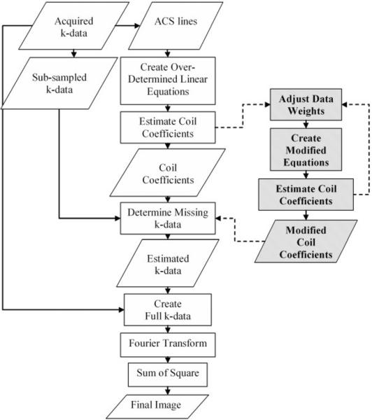
Flowchart of regular GRAPPA and Robust GRAPPA. The input is the acquired k-data which includes the sub-sampled k-data in outer k-space and the ACS lines in center k-space, and the output is the final reconstructed image. As compared to regular GRAPPA, data weights were added for robust estimation, as shown on the right. The robust process is iterative for the case of Slow Robust GRAPPA.

In regular GRAPPA the first step is to create the over-determined linear equations from the ACS lines and estimate the coil coefficients by solving the equations with a least-squares algorithm (Fig. 1). To create the linear equations, blocks of ACS signals from all coils are used to fit a single ACS line in one coil. Each block is composed of one line of measured signal and (ORF)-1 lines of target signal. This process can be represented by the linear equations:

$$S_j^{\mathit{ACS}}(k_y+m\Delta k_y)=\sum _{l=1}^L\sum _{b=1}^4{n}_{j,b,l}^m{S}_l(k_y+b(\mathit{ORF}\left)\Delta k_y\right)$$ [1]

where j is the index of the target coil (j = 1,2,…,L), l is the index of the L coils, b is the index of the block (b = 1–4, we include four blocks), n refers to the coil coefficients, and S refers to the measured signals. With known S and target signal S^ACS, the coil coefficients n are obtained using a pseudo-inverse matrix operation. Equation [1] is applied to each of the L target coils.

The second step is to determine the missing k-space data in outer k-space. To do this, one simply applies the same equation at a different k-space location, using known coil coefficients and the subsampled k-space data to determine the unknown target signals. That is, one can reconstruct the missing k-space lines by direct matrix multiplication.

The final full k-space data are created by combining the estimated missing k-space data and the acquired k-data. After Fourier transform, the sum-of-square method is usually used to create the final image, as shown in Fig. 1.

In GRAPPA, every data point in the ACS region gives an equation. Using a least-squares method to solve the overdetermined equations, regular GRAPPA considers every data point equally.

Slow Robust GRAPPA

In Robust GRAPPA we assign and adjust the data weights in the estimation equations. With the data weights added, Eq. [1] becomes:

$$S_j^{\mathit{ACS}}(k_y+m\Delta k_y)=\sum _{l=1}^L\sum _{b=1}^4{W}_j{n}_{j,b,l}^m{S}_l(k_y+b(\mathit{ORF}\left)\Delta k_y\right)$$ [2]

For each data point in the ACS region, a data weight W is assigned based on the “similarity” of this point with all the other data points. As shown on the right side of Fig. 1, the new method adjusts the data weights of linear equations and improves the accuracy of the estimated coil coefficients. We call this method Robust GRAPPA.

One approach to adjust the weights is to use the “iteratively reweighted least-squares algorithm” (10). It is implemented in robustfit.m, a standard MatLab (MathWorks, Natick, MA) routine in the statistics tool-box. In the algorithm a first regular least- squares fitting is first carried. The residuals of the fitting R are calculated after the fitting, and the weights W in Eq. (2) for the next iteration are determined by a bi-square function:

$$W=\{\begin{array}{cc}{(1-r^2)}^2\hfill & \text{when abs(r)}<1\hfill \\ -{(1-r^2)}^2\hfill & \text{when abs(r)}\ge =1\hfill \end{array}\phantom{\}}$$ [3]

where

$$r=\frac{R}{4.685\ast \left(\frac{\mathit{MAD}}{0.6745}\right)\ast \sqrt{1-h}}$$ [4]

R is the residuals, MAD is the median absolute deviation of the residuals from their median, and h is the leverage value from the least-square fit. The weights W are assigned to the data points and a new least-square fitting is calculated. This process iterates until W do not change or a maximum iteration (500) is achieved.

Effectively, “outliers” are given less weight in the final estimation and the fitting accuracy is improved. Since it is an iterative algorithm, this process is very time-consuming. We call it Slow Robust GRAPPA.

Fast Robust GRAPPA

This simplified approach computes quickly. An initial least-squares fit is performed and the residuals R are calculated and sorted. The weights W is then determined by:

$$\mathit{W}=\{\begin{array}{cc}0\hfill & \text{if}\mathit{R}\text{is in the top}\mathit{m}\%\text{of all the residuals}\hfill \\ 1\hfill & \text{if}\mathit{R}\text{is not in the top}\mathit{m}\%\text{of all the residuals}\hfill \end{array}\phantom{\}}$$ [5]

The data with the largest residuals are labeled as “outliers” data. An “outlier ratio” m is specified by the user (varies from 0% to 20%). With the new data weights W, another least-squares fit is performed, giving the final estimation of coil coefficients. In this method, instead of hundreds of least-square fits, the least-squares operation is done only twice. It is much faster than Slow Robust GRAPPA, and we call it Fast Robust GRAPPA.

Perceptual Difference Model

We use PDM to quantitatively evaluate the reconstructed image quality. PDM is a computerized human vision model that calculates the visual difference between a “test image” and a “gold standard image,” the latter being generated from a full k-space acquisition in our case. PDM has been shown to correlate well with human observers in a variety of MR experiments, including spiral imaging (8), parallel imaging (6,9), and keyhole imaging (7). PDM calculates the “perceptual” difference between a reference image, which is reconstructed with full-sampled k-space data using a sum-of-square method, and a test image, which is reconstructed with subsampled k-space data using regular or Robust GRAPPA method. PDM score represents the image quality of the test image, and lower PDM score indicates better image quality. The detailed structure of the PDM was described in Ref. (7) and the validation experiments for this study are described in the Appendix.

Experiments

With the help of PDM, we systematically evaluated and optimized the Robust GRAPPA techniques. In all, 10,800 test images were generated with a variety of independent variables: MR image datasets, ORF, total reduction factor (TRF), noise level, outlier ratio, and k-space center filling options (Tables 1, 2). The six MR datasets were purposely different. They were acquired with different coils and scanners, and the number of coils, the image size, and image content varied (Table 1).

Table 1.

Image Datasets Used in the Experiments

Datasets	Size	Coils	Contents	Vendor	Field
D1	256×256	4	Head	GE	1.5T
D2	256×256	8	Spine	GE	3T
D3	256×256	4	Head	Siemens	1.5T
D4	256×256	4	Head	Siemens	1.5T
D5	209×256	8	Heart	Siemens	1.5T
D6	256×256	4	Liver	Siemens	1.5T

Table 2.

Independent Variables for Image Reconstruction

Variables	Values
Dataset		D1, D2, D3, D4, D5, D6
TRF (ORF)	1.5, 1.6, 1.7, 1.8	1.9, 2.0, 2.2, 2.4, 2.6	2.8, 2.9, 3.0, 3.1, 3.2, 3.3
	2	3	4
Outlier Ratio		0, 0.01, 0.02, 0.03, 0.04, 0.06, 0.08, 0.1, 0.15, 0.2
Center Filling		Fill, non-fill
Noise		5 dB, 10 dB, 15 dB, 20 dB, 50 dB, no adding noise

Images were reconstructed from downsampled k-space data with different reduction factors. For the peripheral k-space, k-space data were decimated by ORF, that is, we used only one k-space line every other (ORF-1) lines for the reconstruction. For the center k-space (in phase-encoding direction), full-sampled data were used to calculate the sensitivity information. The total acquisition time saved was reflected by TRF, the total number of k-space lines used for reconstruction divided by the number of all PE lines.

In order to test the performance of the reconstruction algorithms under the low-signal-to-noise ratio (SNR) conditions, Gaussian distributed white noise was added to both the real and imaginary channels of the original k-space data. Six different noise levels were tested (Table 2).

The outlier ratio only applied to Fast Robust GRAPPA. A ratio of 0.01 represented that 99% of the original data were used to calculate the coil coefficients. When the outlier ratio was set to be 0, 100% of the original data was used, which made the Robust GRAPPA return to the regular GRAPPA reconstruction. In our experiment, 10 different outlier ratios were tested.

As shown in Fig. 1, in GRAPPA reconstruction the center k-space data (ACS lines) could be used for two purposes: to calculate the coil coefficients and to fill/replace the center final reconstruction matrix to improve the image quality. For the second purpose, people may choose to fill the center k-space or not, based on different considerations (11).

In order to compare reconstruction algorithms over a wide variety of test images, we computed the PDM ratio, obtained by dividing the PDM score of Robust GRAPPA, to that of regular GRAPPA. A PDM ratio smaller than 1 indicated an improvement of image quality with Robust GRAPPA. PDM ratios were computed over all noise and TRF combinations.

Before the exhaustive tests were performed on the Fast Robust GRAPPA, the Fast and Slow Robust GRAPPA reconstruction methods were compared with 48 selected test images. Variables are listed in Table 3. For Slow Robust GRAPPA we used the standard MatLab routine robustfit.m with all the default settings. For Fast Robust GRAPPA an outlier ratio of 0.08 was set just for this comparison. A paired t-test was used to testify if there was significant difference between the Slow and Fast Robust GRAPPA reconstruction.

Table 3.

Independent Variables for Algorithm Comparison

Variables	Values
Algorithm	Slow and Fast Robust GRAPPA
Dataset	D1, D2, D3, D4, D5, D6
TRF (ORF)	1.7		3.0
	2		4
Center Filling	Fill, non-fill
Noise	20 dB, no adding noise

RESULTS

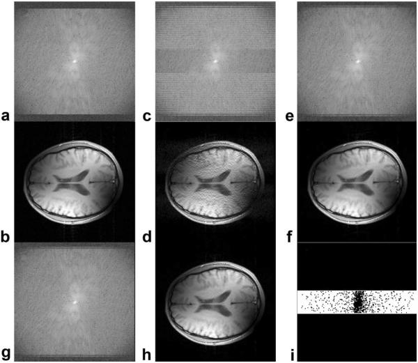
Examples are shown in Fig. 2 (dataset D1, TRF = 2.5, no added noise). Reconstructed images and k-space data from a randomly selected coil (Coil #3) were compared with the original data. As compared with regular GRAPPA, the Robust GRAPPA techniques reduced both noise and artifacts. One could see little difference between the Slow and Fast techniques with regard to both reconstructed image and k-space data. Figure 2i clearly shows the location of the points (outliers) that were eliminated by the Fast Robust GRAPPA reconstruction.

Figure 2.

Example results using different reconstruction methods. The log of the original k-space magnitude data from one of the coils in dataset D1 is shown in (a); the corresponding image is shown in (b). Using a reduction factor of 2.5, regular GRAPPA reconstructed k-space and image data are shown in (c) and (d), respectively. Slow Robust GRAPPA gives improved k-space results in (e) and (f). Fast Robust GRAPPA gives very similar results in (g) and (h), using an outlier ratio of 0.1. Points eliminated in Fast Robust GRAPPA are shown in (i) as black points.

We compared Slow and Fast Robust GRAPPA over all of the 48 test image pairs described in Experiments. A paired t-test indicated that no significant image quality difference exist between Slow and Fast Robust GRAPPA (P = 0.246). Anecdotal visual evaluation of paired images did not find noticeable differences either. The Fast method computed much faster than the Slow method. Therefore, in the following parts of the article we only consider Fast Robust GRAPPA and call it Robust GRAPPA.

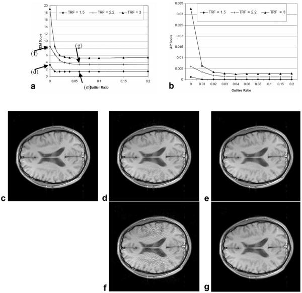
PDM scores and sample images were shown as the function of outlier ratio and TRF (Fig. 3a). Obvious improvements were observed with Robust GRAPPA, with regard to both PDM and visual inspection, at both high and low TRFs. This improvement was also reflected with another popular image quality metric called artifact power (Fig. 3b). Optimal outlier ratio was achieved at 0.08. However, one can see from the figure that outlier ratios over a large range (0.01–0.15) give very similar image quality. The results in Fig. 3 were from dataset D1 and other datasets gave similar results.

Figure 3.

Performance of Robust GRAPPA as a function of outlier ratio and total reduction factor (TRF). Plots of PDM (a) and artifact power (b) show that image quality depends relatively little on outlier ratio when it is larger than 0.01. Images are: (c) reference, giving a PDM of 0; (d) and (f), standard GRAPPA reconstruction for TRF = 1.5 and 2.2, respectively; (e) and (g), corresponding Robust GRAPPA. Conditions are: dataset D1, no added noise, and center k-space filling.

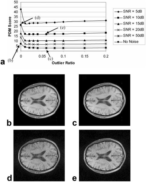
In Fig. 4 Robust GRAPPA reconstructions under different SNRs for dataset D1 were shown, with ORF = 3 and TRF = 2. There were clear improvements as compared to regular GRAPPA, in both high (50 dB) and low SNR (20 dB) conditions. Interestingly, the optimum outlier ratio changed from 0.08–0.01 as SNR decreased from 50 dB to 5 dB.

Figure 4.

Performance of Robust GRAPPA as a function of noise and outlier ratio. Images are: (b) and (d), regular GRAPPA reconstruction for SNR = 50 dB and 20 dB, respectively; (c) and (e), corresponding Robust GRAPPA. Conditions are: data-set D1, TRF = 2 (ORF = 3), and center k-space filling. Robust GRAPPA outperforms regular GRAPPA in both high and low SNR conditions. Note the 50 dB line are overlapped with the no-noise line in the figure.

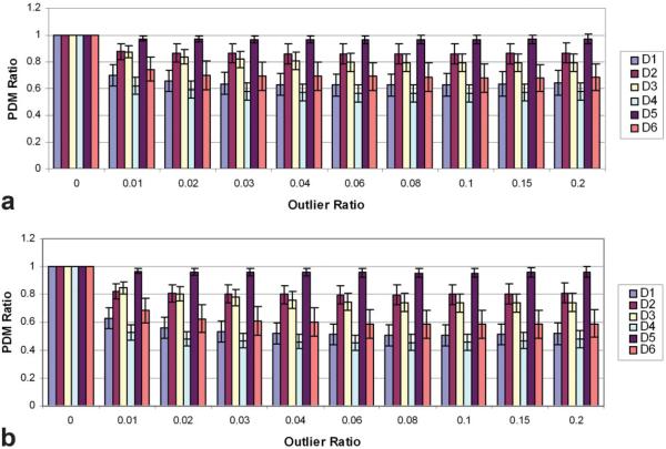
In Fig. 5 the overall performance of Robust GRAPPA was plotted with different image datasets and outlier ratios. PDM ratios were statistically significant lower than 1 for all six datasets (P < 0.005), proving the advantages of the Robust GRAPPA technique. This result held with (Fig. 6a) or without (Fig. 6b) ACS filling. The improvement in the image quality was more obvious for datasets D1, D2, D3, D4, and D6. Improvement for D5 was not significant. The overall best outlier ratio was achieved when we set the outlier ratio as 0.08, although the change around 0.08 was comparably flat.

Figure 5.

PDM ratios with (a) and without (b) center filling. The PDM ratio is the PDM score with Robust GRAPPA divided by the PDM with regular GRAPPA. Each datum point in the figure represents the average PDM ratio over 90 images (15 different TRFs and 6 levels of noise). Error bars correspond to one standard deviation. Robust GRAPPA generally outperformed regular GRAPPA for both center-filling options.

Figure 6.

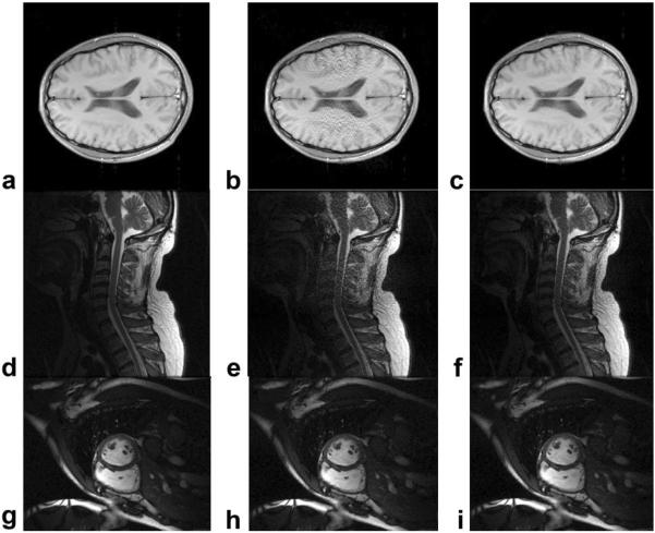
The image quality comparisons between the Regular GRAPPA (second column) and Robust GRAPPA (third column) for dataset D1 (first row), D2 (second row), and D5 (third row). Images reconstructed with full k-space were provided as references (first column). No noise was added, and all images were with center filling. Total reduction factor was 2.2 with the reduction factor of 3. For Robust GRAPPA reconstruction, outlier ratio was set as 0.08.

The final reconstructed images are shown in Fig. 6 for dataset D1, D2, and D5. For each dataset three images are shown: the image reconstructed with full data (6a,d,g), with regular GRAPPA (6b,e,h), and with Robust GRAPPA (6c,d,i). No additional noise was added and total reduction factor was set to 2.2 (reduction factor = 3). ACS lines were filled into final k-space data to improve the image quality. One can see that very obvious improvement was observed for D1 and D2 with the Robust GRAPPA techniques. The improvement was not obvious for dataset D5, as shown in Fig. 5.

DISCUSSION

The Robust GRAPPA algorithm improved the accuracy of the coil coefficients estimation and reconstructed image quality. With the help of PDM we were able to do extensive testing of Robust GRAPPA, creating 10,800 test images. Robust GRAPPA outperformed regular GRAPPA for both low and high TRFs (Fig. 3), and both low and high noise conditions (Fig. 4). Improvement was observed from all five datasets tested (Fig. 5). Both Fast and Slow Robust GRAPPA gave similar improvements and the Fast method computed in less than 1/10 of the time of the Slow method. The Fast method usually added only a little extra computational time to regular GRAPPA, depending on the number of ACS lines and number of coils. With the Fast method we found that image quality was relatively insensitive to outlier ratio, and a value of 8% was about optimal (Fig. 5). Low SNR favored lower outlier ratios (Fig. 4), but the value of 8% was still quite reasonable.

We can consider our modification of GRAPPA with regard to other modifications in the literature, following the original 2002 publication (3). Park et al (12) proposed a limited calibration region in both the frequency- and phase-encoding directions to remove the artifact and noise effects in GRAPPA reconstruction. Our method eliminated outliers based on the image content, and could be robust on different coils and calibration region locations. As we can see in Fig. 2(i), more outliers were removed from the center of k-space. This observation agreed with the results of the Park et al article. Similarly, Qu et al (13) proposed tailoring the acquired k-space points for the GRAPPA reconstruction. This scheme automatically selected the k-space subset points and improved the accuracy of coil coefficients estimation. In view of the overdetermined linear equations, this algorithm actually reduced the number of rows of the inverse matrix, while Robust GRAPPA reduced the number of columns. Robust GRAPPA should be a good complement for Tailored GRAPPA, because when the signal redundancies decreased with Tailored GRAPPA the effects of outliers will be increased. A combination of these two algorithms could further improve the accuracy of coil coefficients estimation and image quality. Tailored GRAPPA could be first applied to select the optimal subset points and Robust GRAPPA could then be applied to remove the effects from outliers. The use of overdetermined condition in parallel imaging could be also found in Ref. (14), where it was applied to SENSE algorithm to remove the image artifact.

In GRAPPA the least-square fitting usually ensures a fit to the high SNR points near the center of k-space, but not to the overall ACS region. That is, the center k-space data have a larger influence on results. When the robust fitting method was applied, outliers were more likely to concentrate in the center k-space, as seen in Fig. 2i. Removing them greatly improves the fitting accuracy and image quality. Outlier, “bad” data, can be generated for various reasons. Noise and low sensitivity could be important factors. Flow and nonrigid motion introduce inconsistency in the k-space data; signal decays including T2 and T2* effects and off-resonance artifacts can be contributors. In addition, we believe that the fact that the small GRAPPA kernel cannot fully represent the coil sensitivity information is another important reason.

The concentration of outliers in center k-space can partly explain why the optimal outlier ratio is reduced when data SNR is reduced (Fig. 4). In a high SNR condition, peripheral k-space data could provide a good estimation; thus, removing more outliers in the center is beneficial. When the noise level increases the peripheral data become unreliable; thus, using more high-quality center k-space data is desirable.

The basic idea of Robust GRAPPA lies in the weighted estimation of the GRAPPA interpolation kernel, thus improving the fitting accuracy and final image quality. It removes outliers and makes the fitting process more robust. From another point of view, regular GRAPPA is a “Least-Squares Regression” (L2 norm). Robust GRAPPA can become a “Least Absolute Deviations Regression” (L1 norm) when certain weights are applied in Eq. [2]. An L1 norm is more robust to outliers, but it is known to lose some stability, something we observed in image reconstruction experiments. A limited number of iterations in Slow Robust GRAPPA with the bi-square function as the weights effectively reduce the effects of outliers, while keeping the stability of regression. Our preferred ad hoc solution, Fast Robust GRAPPA, removes a percentage of outliers, gives very stable results, and does so with much less computational demand.

As compared to other potential methods, the “Fast Robust” method was greatly simplified. We marked outliers in a single step based on their residuals and essentially eliminated them from further consideration. Although we found insignificant difference between the Fast and Slow methods, it might be worthwhile to further investigate algorithmic alternatives. In addition to the robust methods described in Experiments, we could use more complex methods to locate outliers (15–17). Once outliers were located, as an alternative to assigning zero or positive data weights, negative or even complex data weights could be used.

In this study the perceptual difference model again proved its ability and adequacy to evaluate the image quality of fast MR imaging. PDM scores faithfully represented the perceived image quality of the thousands of images generated by the combination of different reconstruction methods, parameters, or noise levels. By quantifying image quality accurately by a scalar value, one could better see the change of image quality with some particular parameters. One could also apply statistical methods to analyze these scores and make the conclusions more convincing. It could also be used as a metric for parameter optimization.

Instead of PDM, some researchers used “artifact power” to represent the difference between a reference image and a test image (12). Artifact power is actually a transformation of the popular metric, mean squared error (MSE). MSE is very simple and direct, and it is widely used by researchers. However, it is a physical measurement of the difference, and the human visual perceptual characteristics are completely ignored. As proved in Refs. (9,18) and in the Appendix of this article, PDM could better represent the human subjects' responses to the image quality. For the Robust GRAPPA algorithm presented here the improvement was very obvious, and one could tell the difference just from the visual inspections. In this case, similar results would be achieved even if artifact power or MSE were used as the evaluation method (Fig. 3b). However, for applications where a subtle difference is important, PDM is strongly recommended.

Finally, it is important to point out that Robust GRAPPA applies to non-Cartesian sampling, where GRAPPA has already been demonstrated to work: eg, spiral (19), radial (20), PROPELLER (21), etc. It would be applicable to dynamic imaging (22) and 3D imaging (23) too. Once again, we believe that PDM is very suitable for evaluation in these applications.

In conclusion, a new modification of GRAPPA reconstruction has been proposed and optimized. Our results showed that Robust GRAPPA effectively improved the reconstructed image quality compared with regular GRAPPA. PDM was helpful in designing and optimizing the MR reconstruction algorithms.

APPENDIX

Structure and Experiment of PDM

The quality of the reconstructed images was evaluated with the PDM. The model was inspired by the visible differences predictor (VDP) model reported by Daly (24), but we have made multiple modifications over the years. It has been validated for the evaluation of other fast MRI applications and described in detail in previous articles (7–9).

We performed a human observer experiment on representative test images and compared the results with PDM. Human observers were asked to evaluate the quality of selected images using a modified double-stimulus continuous quality-scale (DSCQS) test (25), which is very similar to that previously reported by Salem et al (7) and by Martens and Meesters (26) on a similar model used for other purposes. The same validation experiment was applied in Ref. (9), with a different test image dataset.

To test the full range of image quality in our images, 40 test images were selected with PDM scores uniformly spread from best to worst, all from the reconstructed images of dataset D5 (Table 1). The 40 images were presented to three subjects, one of the authors and two image processing experts. The experiment was done using a MatLab program, which included a GUI input for recording scores using a slider or keyboard. Each presentation consisted of a two-panel display, with the high-quality reference image and a randomly selected test image on the left and right, respectively. Observers were instructed to score the general quality of the test image on a scale of 100 to 0, with 0 being the best quality and 100 being the worst quality. Observers were aware that the reference image has the “best” image quality and that they should have a score of 0. Observers performed a training session on at least 30 images spanning a wide range of image quality to help calibrate them for the experiment. During this time subjects were free to ask questions of the first author. Another set of test images was then used for the experiment. To account for intraobserver differences, each of the 40 test images was displayed and evaluated twice. The experiment was carried out in a darkened room and normally took 1 hour. A perceptually linearized, high-quality gray scale monitor was used. There was no time limitation and subjects were allowed to revise their results, including back-tracking, at any time. Informed consent was obtained before the experiment.

Data were processed before comparisons to PDM. First, two scores given to the same test image from the same subject were averaged to reduce the intraobserver difference. To compensate for scale boundary effects, a nonlinear scale transformation (25) was used, which normalizes data based on the middle and extreme values in the data.

We compared PDM scores to processed human subject ratings and the results are shown in Fig. 7. Average human observer scoring of image quality was highly correlated with PDM scores (R = 0.91, P < 0.001). Reduced correlation was obtained using the mean-squared-error (MSE) as the image quality metric (R = 0.89, P < 0.001).

Figure 7.

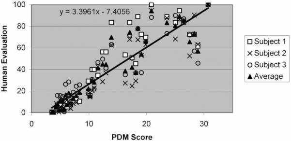
Human subject experiment data were analyzed and compared to PDM. Each datum represents a score for one subject on one of the test images, with its PDM score on the x-axis. Human scoring is normalized as described in the text. A high correlation (R = 0.914) exists between the average human evaluation and PDM scores. The x-axis intercept (2.17) corresponds to a value where people perceived the images to have the same image quality.

REFERENCES

- 1.Pruessmann KP, Weiger M, Scheidegger MB, Boesiger P. SENSE: sensitivity encoding for fast MRI. Magn Reson Med. 1999;42:952–962. [PubMed] [Google Scholar]
- 2.Sodickson DK, Manning WJ. Simultaneous acquisition of spatial harmonics (SMASH): fast imaging with radiofrequency coil arrays. Magn Reson Med. 1997;38:591–603. doi: 10.1002/mrm.1910380414. [DOI] [PubMed] [Google Scholar]
- 3.Griswold MA, Jakob PM, Heidemann RM, et al. Generalized auto-calibrating partially parallel acquisitions (GRAPPA) Magn Reson Med. 2002;47:1202–1210. doi: 10.1002/mrm.10171. [DOI] [PubMed] [Google Scholar]
- 4.Griswold MA, Jakob PM, Nittka M, Goldfarb JW, Haase A. Partially parallel imaging with localized sensitivities (PILS) Magn Reson Med. 2000;44:602–609. doi: 10.1002/1522-2594(200010)44:4<602::aid-mrm14>3.0.co;2-5. [DOI] [PubMed] [Google Scholar]
- 5.Pruessmann KP, Weiger M, Bornert P, Boesiger P. Advances in sensitivity encoding with arbitrary k-space trajectories. Magn Reson Med. 2001;46:638–651. doi: 10.1002/mrm.1241. [DOI] [PubMed] [Google Scholar]
- 6.Jiang YH, Huo DL, Wilson DL. Methods for quantitative image quality evaluation of MRI parallel reconstructions: detection and perceptual difference model. Magn Reson Imaging. 2007;25:712–721. doi: 10.1016/j.mri.2006.10.019. [DOI] [PubMed] [Google Scholar]
- 7.Salem KA, Lewin JS, Aschoff AJ, Duerk JL, Wilson DL. Validation of a human vision model for image quality evaluation of fast interventional magnetic resonance imaging. J Electron Imaging. 2002;11:224–235. [Google Scholar]
- 8.Huo D, Salem KA, Jiang Y, Wilson DL. Optimization of spiral MRI using a perceptual difference model. Int J Biomed Imaging. 2006;2006 doi: 10.1155/IJBI/2006/35290. Article ID 35290. [DOI] [PMC free article] [PubMed] [Google Scholar]
- 9.Huo DL, Xu D, Liang ZP, Wilson D. Application of perceptual difference model on regularization techniques of parallel MR imaging. Magn Reson Imaging. 2006;24:123–132. doi: 10.1016/j.mri.2005.10.018. [DOI] [PubMed] [Google Scholar]
- 10.Huber PJ. Robust statistics. John Wiley & Sons; New York: 1981. [Google Scholar]
- 11.Huo DL, Griswold MA, Blaimer M, Wilson DL. Potential pitfalls of including reference data in parallel imaging reconstructions at high acceleration. Proc ISMRM, Seattle. 2006:287. [Google Scholar]
- 12.Park J, Zhang Q, Jellus V, Simonetti O, Li DB. Artifact and noise suppression in GRAPPA imaging using improved k-space coil calibration and variable density sampling. Magn Reson Med. 2005;53:186–193. doi: 10.1002/mrm.20328. [DOI] [PubMed] [Google Scholar]
- 13.Qu P, Shen GX, Wang CS, Wu B, Yuan J. Tailored utilization of acquired k-space points for GRAPPA reconstruction. J Magn Reson. 2005;174:60–67. doi: 10.1016/j.jmr.2005.01.015. [DOI] [PubMed] [Google Scholar]
- 14.Winkelmann R, Bornert P, Dossel O. Ghost artifact removal using a parallel imaging approach. Magn Reson Med. 2005;54:1002–1009. doi: 10.1002/mrm.20640. [DOI] [PubMed] [Google Scholar]
- 15.Atkinson AC. Fast very robust methods for the detection of multiple outliers. J Am Stat Assoc. 1994;89:1329–1339. [Google Scholar]
- 16.Fung WK. Unmasking outliers and leverage points — a confirmation. J Am Stat Assoc. 1993;88:515–519. [Google Scholar]
- 17.Hadi AS, Simonoff JS. Procedures for the identification of multiple outliers in linear-models. J Am Stat Assoc. 1993;88:1264–1272. [Google Scholar]
- 18.Girod B. What's wrong with mean-squared error? In: Watson AB, editor. Digital images and human vision. MIT Press; Cambridge, MA: 1993. pp. 207–220. [Google Scholar]
- 19.Heberlein K, Hu XP. Auto-calibrated parallel spiral imaging. Magn Reson Med. 2006;55:619–625. doi: 10.1002/mrm.20811. [DOI] [PubMed] [Google Scholar]
- 20.Arunachalam A, Samsonov A, Block WF. Self-calibrated GRAPPA method for 2D and 3D radial data. Magn Reson Med. 2007;57:931–938. doi: 10.1002/mrm.21223. [DOI] [PubMed] [Google Scholar]
- 21.Blaimer M, Barkauskas K, Kannengiesser S, et al. Artifact reduction in undersampled BLADE/PROPELLER MRI by k-space extrapolation using parallel imaging. Proc ISMRM, Seattle. 2006:5. [Google Scholar]
- 22.Breuer FA, Kellman P, Griswold MA, Jakob PM. Dynamic autocalibrated parallel imaging using temporal GRAPPA (TGRAPPA) Magn Reson Med. 2005;53:981–985. doi: 10.1002/mrm.20430. [DOI] [PubMed] [Google Scholar]
- 23.Breuer FA, Blaimer M, Mueller MF, et al. Controlled aliasing in volumetric parallel imaging (2D CAIPIRINHA) Magn Reson Med. 2006;55:549–556. doi: 10.1002/mrm.20787. [DOI] [PubMed] [Google Scholar]
- 24.Daly S. The visual differences predictor: an algorithm for the assessment of image fidelity. In: Watson AB, editor. Digital images and human vision. MIT Press; Cambridge, MA: 1993. pp. 179–206. [Google Scholar]
- 25.Union IT. Recommendation ITU-R BT 500-7: methodology for the subjective assessment of the quality of television pictures. International Telecommunication Union; Geneva: pp. 1974–1997. [Google Scholar]
- 26.Martens JB, Meesters L. Image dissimilarity. Signal Process. 1998;70:155–176. [Google Scholar]