Significance
Most statistical analyses involve some kind of ‟selection”—searching through the data for the strongest associations. Measuring the strength of the resulting associations is a challenging task, because one must account for the effects of the selection. There are some new tools in selective inference for this task, and we illustrate their use in forward stepwise regression, the lasso, and principal components analysis.
Keywords: inference, P values, lasso
Abstract
We describe the problem of “selective inference.” This addresses the following challenge: Having mined a set of data to find potential associations, how do we properly assess the strength of these associations? The fact that we have “cherry-picked”—searched for the strongest associations—means that we must set a higher bar for declaring significant the associations that we see. This challenge becomes more important in the era of big data and complex statistical modeling. The cherry tree (dataset) can be very large and the tools for cherry picking (statistical learning methods) are now very sophisticated. We describe some recent new developments in selective inference and illustrate their use in forward stepwise regression, the lasso, and principal components analysis.
Statistical science has changed a great deal in the past 10–20 years, and is continuing to change, in response to technological advances in science and industry. The world is awash with big and complicated data, and researchers are trying to make sense out of it. Leading examples include data from “omic” assays in the biomedical sciences, financial forecasting from economic and business indicators, and the analysis of user click patterns to optimize ad placement on websites. This has led to an explosion of interest in the fields of statistics and machine learning and spawned a new field some call “data science.”
In the words of Yoav Benjamini, statistical methods have become “industrialized” in response to these changes. Whereas traditionally scientists fit a few statistical models by hand, now they use sophisticated computational tools to search through a large number of models, looking for meaningful patterns. Having done this search, the challenge is then to judge the strength of the apparent associations that have been found. For example, a correlation of 0.9 between two measurements A and B is probably noteworthy. However, suppose that I had arrived at A and B as follows: I actually started with 1,000 measurements and I searched among all pairs of measurements for the most correlated pair; these turn out to be A and B, with correlation 0.9. With this backstory, the finding is not nearly as impressive and could well have happened by chance, even if all 1,000 measurements were uncorrelated. Now, if I just reported to you that these two measures A and B have correlation 0.9, and did not tell which of these two routes I used to obtain them, you would not have enough information to judge the strength of the apparent relationship. This statistical problem has become known as “selective inference,” the assessment of significance and effect sizes from a dataset after mining the same data to find these associations.
As another example, suppose that we have a quantitative value y, a measurement of the survival time of a patient after receiving either a standard treatment or a new experimental treatment. I give the old drug (1) or new drug (2) at random to a set of patients and compute the mean difference in the outcome , where s is an estimate of SD of the raw difference. Then I could approximate the distribution of z by a standard normal distribution, and hence if I reported to you a value of, say, you would be impressed because a value that large is unlikely to occur by chance if the new treatment had the same effectiveness as the old one (the P value is about 1%). However, what if instead I tried out many new treatments and reported to you only ones for which ? Then a value of 2.5 is not nearly as surprising. Indeed, if the two treatments were equivalent, the conditional probability that exceeds 2.5, given that it is larger than 2, is about 27%. Armed with knowledge of the process that led to the value , the correct selective inference would assign a P value of 0.27 to the finding, rather than 0.01.
If not taken into account, the effects of selection can greatly exaggerate the apparent strengths of relationships. We feel that this is one of the causes of the current crisis in reproducibility in science (e.g., ref. 1). With increased competiveness and pressure to publish, it is natural for researchers to exaggerate their claims, intentionally or otherwise. Journals are much more likely to publish studies with low P values, and we (the readers) never hear about the great number of studies that showed no effect and were filed away (the “file-drawer effect”). This makes it difficult to assess the strength of a reported P value of, say, 0.04.
The challenge of correcting for the effects of selection is a complex one, because the selective decisions can occur at many different stages in the analysis process. However, some exciting progress has recently been made in more limited problems, such as that of adaptive regression techniques for supervised learning. Here the selections are made in a well-defined way, so that we can exactly measure their effects on subsequent inferences. We describe these new techniques here, as applied to two widely used statistical methods: classic supervised learning, via forward stepwise regression, and modern sparse learning, via the “lasso.” Later, we indicate the broader scope of their potential applications, including principal components analysis.
Forward Stepwise Regression
Supposed that we have a dataset with N observations , being the outcome measurement and each a vector of p predictors (or features). We wish to build a model for predicting from . This is known as the supervised learning problem, because the outcome y supervises (or guides) the prediction process.† The standard linear regression model has the form
| [1] |
with the errors being independent and distributed as , where β is a vector of p unknown coefficients (weights) to be estimated.
With a moderate or large number of predictors, it is common to use forward stepwise regression to select a good subset of predictors. This procedure enters predictors one at a time, choosing the predictor that most decreases the residual sum of squares at each stage ( being the predicted value for observation i). Classic statistical theory for assessing the strength each predictor would go as follows. Defining to be the residual sum of squares for the model containing k predictors, we use the change in residual sum of squares to form a test statistic
| [2] |
(with σ assumed known here), and compare it to a χ2 distribution with one degree of freedom. There is a big problem with this approach, however. This classic theory assumes that the models being compared were prespecified before seeing the data. However, this is clearly not the case here: We have “cherry-picked” the best predictor at each stage to maximize . Hence, we would expect that even if the new predictor had no effect in the population, the distribution of values of will be larger than a distribution.
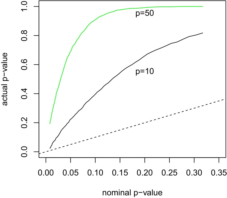
Fig. 1 quantifies this. With a sample size of , we simulated Gaussian datasets from two scenarios: one with predictors and the other with . There is no signal in the underlying population. We are examining just the first step of forward stepwise regression. The horizontal axis shows the nominal (desired) P value (set by the statistician) and the vertical axis is the actual P value from this process, which properly accounts for the selection of the best predictor among the p. For , we see that, for example, a test at nominal type I error of 5% would actually have a type I error of 20%. For , things become worse: The actual type I error is about 70%.
Fig. 1.
A simulation example with observations and or 50 predictors and null effects (). Shown are the nominal and actual P values for entering the strongest predictor at the first step; the 45° dashed line is included for reference.
The correct P values in Fig. 1 were estimated by simulating from the Gaussian distribution and recording the maximal value for achieved each time. However, we would like to obtain a correct P value not just for the first step of forward stepwise regression, but for all steps.
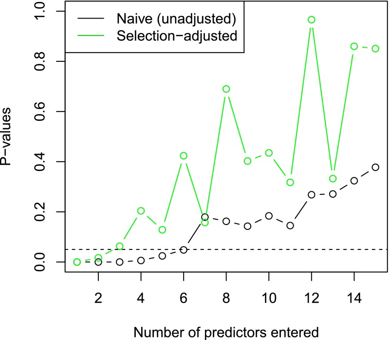
As an example, Rhee et al. (2) studied six nucleoside reverse transcriptase inhibitors that are used to treat HIV-1. The target of these drugs can become resistant through mutation, and Rhee et al. (2) compared a collection of models for predicting the log susceptibility, a measure of drug resistance based on the location of mutations. We chose one of the inhibitors, with a total of samples and mutation sites. To make the problem more manageable computationally, we randomly selected 100 of the samples and chose the 30 sites with highest variation in mutation status across all samples. Forward stepwise regression entered the predictors in the order . Fig. 2 gives a summary of the P values.
Fig. 2.
P values for HIV data, as predictors are entered successively into the model by forward stepwise regression .The black points are the naive P values that do not correct of the selection effects, and the green points are selection-adjusted.
The naive P values suggest that there are six strong predictors (P value less than 0.05), but the more realistic selection-adjusted P values yield only two or three significant predictors.
How were these adjusted P values obtained? Trying to obtain them by naive Monte Carlo sampling would be tedious, and perhaps infeasible for a large number of predictors, because we would have to generate many samples and keep only those for which the sequence of selected variables is the same as that obtained in our original data. Fortunately, there is a simple mathematical construction that gives us these selection-adjusted P values in closed form.
Recall that our data vector y is normally distributed with mean and variance . Consider again the HIV data and suppose that we have taken two steps of forward stepwise regression, entering the variables and . Assume that we are interested, for example, in the true partial regression coefficient of in this model. Then, our estimate would be the least squares coefficient of in the fitted model. Standard statistical theory would tell us that has a normal distribution with mean β and some variance :
| [3] |
However, this theory assumes that we had only these two predictors available to us at the onset. This is not the case here, because we have actually selected the strongest two predictors from among the 30 predictors available. This selection should change how we view the strength of the apparent association between and y. In particular, the number of predictors from which we chose these two should affect how we assess the apparent association. If we had started with 300 rather than 30 predictors, we should have set a higher bar for calling significant in our model.
How do we adjust for the effects of selection? It turns out that for forward stepwise regression and many other procedures the selection events can be written in the “polyhedral” form for some matrix A and vector b (3, 4). We can understand this statement as follows. Suppose that we consider any new vector of outcomes, say , in place of our actual data y. We run our forward stepwise procedure and keep track of the predictors entered at each stage. These will not likely be the same as our original list because the data have changed. However, the polyhedral form says that the set of new data vectors that would yield the same list of predictors (up to some step, such as step 2) can be described by the set . The quantities A and b depend on the data and the selected variables. Roughly speaking, each stage of forward stepwise regression represents a competition among all p variables, and A and b simply reconstruct this competition and check whether yields the same result. What does this polyhedral selection give us? It turns out that under the selection the naive expression (Eq. 3) is replaced by a truncated normal distribution:
| [4] |
This is just a normal distribution truncated to lie in the interval , The limits depend on the data and the selection events that led to the model in question. The formulae for these limits are somewhat complicated but are easily computable. Details can be found in refs. 3 and 4. All of this has given us the key result (Eq. 4), which exactly accounts for the selection process through the truncation limits . We used this result to get the selection-adjusted P values in Fig. 1.
Let’s dig more deeply to understand how this works. The limits express the fact that the selection events in forward stepwise regression restrict the possible range of values of that we might obtain after the selection has been made. For example, consider again the second step of forward stepwise regression and let be the regression coefficient for . To simplify matters, suppose that all of the predictors were uncorrelated and standardized to have mean 0 and variance 1. Then, having selected at the first step, we know that the regression coefficient for must be larger than the coefficients of all of the other 28 predictors not yet chosen (because it won the competition and was entered at step 2) and can be no larger than the coefficient of (because the latter won the competition at the first stage). These two facts define the limits c and d, respectively. With correlated predictors—as in our data—the definitions of c and d are more complicated, but the idea is the same.
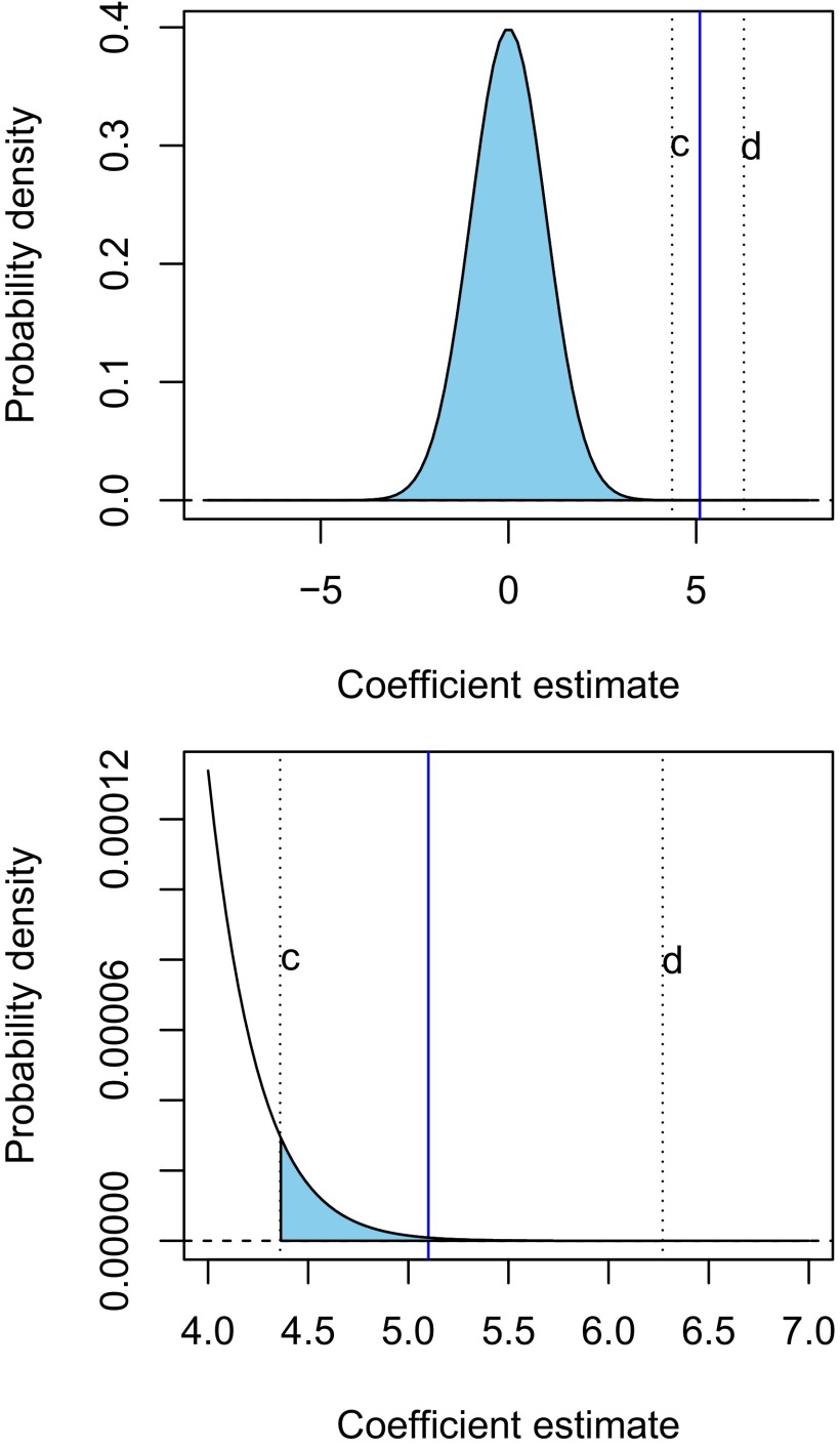
Fig. 3 depicts this situation, showing a truncated normal distribution, with truncation limits .
Fig. 3.
HIV data: truncated normal distribution for the coefficient of , the ninth feature measuring mutation status at a given site. The standardized coefficient for equals 5.1 and is indicated by the vertical blue line in each plot. The truncation limits implied by the selection are . The lower panel zooms in on the area of interest in the tail of the distribution.
Ignoring the selection effects, under the null hypothesis that the true coefficient for was actually 0, and the error variance was 1, then would have a standard normal distribution. Hence we would expect to fall between, say, −2 and +2 and would consider it to be evidence against the null hypothesis if it fell outside this range. Indeed, the observed value of 5.1 would be considered extremely unlikely under the null hypothesis. However, accounting properly for the fact that has been selected at the second stage of forward stepwise regression changes the way in which we judge the observed value of . The selection events imply that the estimate must lie between c and d (4.3 and 6.3 in the Fig. 3, respectively.) Hence, the value of 5.1 represents moderate but not overwhelming evidence that the coefficient is nonzero.
False Discovery Rates and a Sequential Stopping Rule
Looking at the sequence of adjusted P values (green points) in Fig. 1, a natural question arises: When should we stop adding variables? Should we stop at, say, two or three predictors, beyond which the P values are above 0.05? If we do stop there, what can we say about the resulting model? The notion of false discovery rate (FDR) is useful for this purpose. This concept has been an important one for large-scale testing, especially in the biomedical sciences (see ref. 5).
Let’s review this concept and other related, more traditional ones. Table 1 summarizes the theoretical outcomes of m hypothesis tests.
Table 1.
Possible outcomes from m hypothesis tests
| Called not significant | Called significant | Total | |
| true | U | V | |
| false | T | S | |
| Total | R | m |
The quantity V counts false-positive calls, and much of statistical testing focuses on , the probability of at least one false positive. This is called the familywise error rate (FWER), and many statistical methods try to ensure that FWER is less than some level (such as 0.05). This is a useful approach when the number of tests m is not too large (say, <50). However, with a larger number of tests, common in today’s big data problems, we expect that V will be much great than 1 and this approach is too stringent. Instead we shift our focus to the FDR:
| [5] |
This is the average proportion of false-positive calls that we make, among the R tests that we reject, that is, effects that we call significant. (V/R is defined to be zero when R = 0.)
Now, it turns out that there is a simple stopping rule for sequences of P values as in Fig. 1 that gives us automatic control of the FDR of the resulting model (Eq. 6). Choosing a target FDR level of α, and denoting the successive P values by , the ForwardStop rule (ref. 6) is defined by
| [6] |
Essentially, we stop at the last time that the average P value up to that point is below some target FDR level α. This average, however, is taken on the (complementary) log scale. Using the ForwardStop rule, the final model contains the predictors entered at the first steps and has FDR at most α.
In the HIV example, for we get , meaning that we should stop after three steps. If we do so, the expected number of false positives is . Alternatively, if we set , we obtain ; there will be false positives on average.
The Lasso
We now broaden our discussion to a more modern approach to supervised learning, one that can be applied to large datasets. We give a brief description of the method and then show how selective inference can be applied in this more general framework.
The lasso, or penalization, recasts the regression problem as a convex optimization.‡ The lasso solves the problem
| [7] |
The tuning parameter λ effectively balances the tradeoff between two objectives: the goodness of fit to the data (sum squares in the first term) with the complexity of model (second term). It turns out that this is equivalent to minimizing the sum of squares with a “budget” constraint . The value of s depends on λ: Larger values of λ imply a smaller budget s. The best value for λ or s depends on the data and is usually chosen by cross-validation (described below).
Because of the absolute value function appearing in the penalty, over a range of λ values the solution to this problem is sparse, that is, many of the weights are set to 0. Hence, like forward stepwise regression, the lasso selects the most informative predictors among the p available predictors. However, because the problem has been cast as a convex optimization, the search throughout the possible models can be carried out much more effectively. Lasso and penalization methods are now widely used in statistics, engineering, and other sciences, for example in signal processing and compressed sensing (7–9).
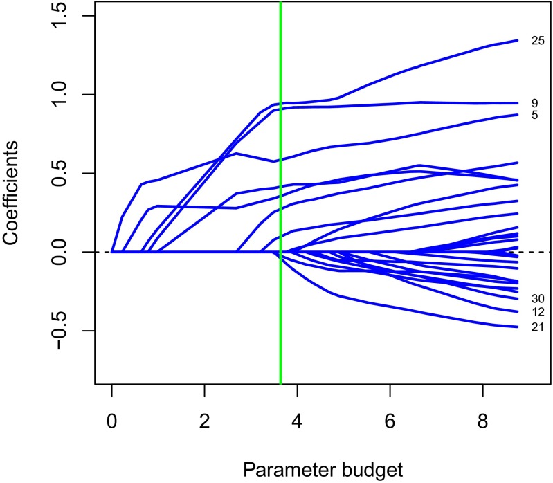
For a fixed choice of the tuning parameter λ, the solution to Eq. 7 has nonzero values on a subset of the predictors, what we call the active set. These are the most informative predictors, as judged by the lasso. Fig. 4 shows the profiles of the solutions to the lasso problem for the HIV data.
Fig. 4.
Paths of estimated coefficients from the lasso applied to the HIV data. Each coefficient path corresponds to the estimated β for a mutation number, with some of mutation site numbers with larger coefficients on the right. The estimated optimal budget is indicated by the vertical green line.
Each profile corresponds to one predictor (mutation site). The different points on each profile correspond to different values of the penalty parameter λ, with this value decreasing as we move from left to right. For interpretability, we have not plotted against λ on the horizontal axis, but the “parameter budget” implied by each value of λ. On the left, λ is very large and the effective budget is zero, so that all parameter estimates are zero. As we move to the right, λ decreases and the effective budget increases, so that more parameters become nonzero. The vertical dotted lines mark the places where a coefficient becomes nonzero, as we move from left to right. On the right, the value of λ is zero so that there is no budget constraint on the parameters. Hence, the values at the right end of the plot are the usual least squares estimates.
Also shown on the plot is the optimal value of λ (green line) estimated using cross-validation. Cross-validation works as follows. (i) We divide the samples into roughly 10 equal-sized parts at random. (ii) For each part K, leave out this part, fit the lasso to the other nine parts over a range of λ values, and then record the prediction error over the left-out part. (iii) Repeat step ii for , and for each value of λ, compute the average prediction error over the 10 parts. Finally our estimate is the value yielding the smallest average prediction error. The cross-validated choice of λ yielded a model with nine predictors (Fig. 4).
It turns out that this selection of predictors can again be described as a polyhedral region of the form . That is, for fixed predictors and value λ, the vector of response values that would yield the same active set after applying the lasso can be written in the form . Here A and b depend on the predictors, the active set and λ, but not y. This fact gives us what we need to construct selection-adjusted intervals for the parameters of the fitted model, using the same arguments as above for forward stepwise regression.
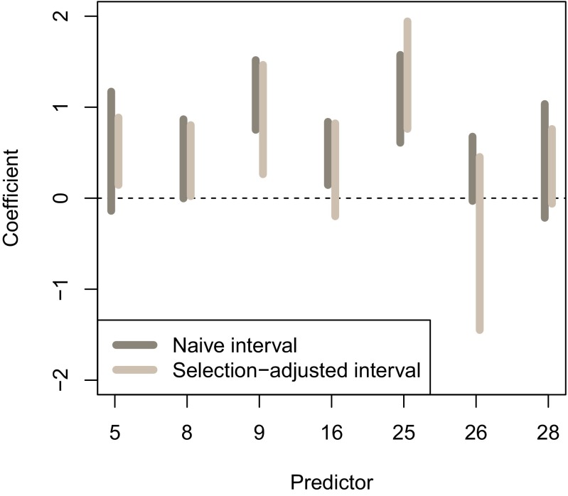
Fig. 5 shows naive least squares confidence intervals and the selection-adjusted intervals for the nine underlying parameters. We see that some of the selection-adjusted intervals are much wider than their naive counterparts.
Fig. 5.
Selection intervals for the HIV data, from the fitted lasso model.
Principal Components and Beyond
Principal components analysis (PCA) is a classic statistical method developed in the early 1900s but now used more widely used than ever. For example, PCA was a core method used by most leading competitors in the Netflix movie prediction competition (10). PCA is a method for unsupervised learning that seeks to discover the important correlation patterns among a set of features. It works by computing the sets of linear combinations of features that are maximally correlated. It can be thought as a method for determining the K leading eigenvectors and eigenvalues of the sample correlation matrix of the features.
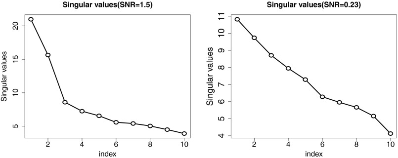
In PCA analysis one computes the leading eigenvectors and eigenvalues (one for each component) and then must decide on the number of components K that are “significant.” Traditionally, this is done through the so-called scree plot, which is simply a plot of the eigenvalues in order from smallest to largest. Fig. 6, Left shows an example from some simulated data with nine features. The underlying correlation matrix, from which the data were simulated, has two strong components.
Fig. 6.
Eigenvalue (scree) plots for two simulated data matrices, each with nine features. (Left) There are two strong leading components in the underlying population. (Right) The two leading components are only moderate in strength.
The scree plot shows a nice “elbow” and would lead us to choose the correct number of components (two). In Fig. 6, Right, we have reduced the signal-to-noise ratio, so that the population eigenvalues of the first two eigenvectors are only moderately larger than the others. Now the scree plot shows no elbow, and we would be hard pressed to guess the number of components.
However, selective inference can come to our rescue. Choosing the leading eigenvectors of a covariance matrix is similar in spirit to forward stepwise regression, and with somewhat more complicated mathematics one can derive selection-adjusted P values for each successive increase in the rank (11). For the example in Fig. 6, Right, the adjusted P values are (0.030, 0.064, 0.222, 0.286, 0.197, 0.831, 0.510, 0.185, and 0.1260), and hence this gives a moderately strong indication of the correct rank. Although this may seem too good to true based on the scree plot, one must remember that the P value estimation procedure uses more information in the correlation matrix than just the eigenvalues shown here.
Discussion
Many, or most, modern statistical methods, in this era of big data, use some form of selection to choose a best-fitting model among a plethora of choices. We have seen two examples above: forward stepwise regression and the lasso. There are many more examples, including methods for time and spatial analysis, interpretation of images, and network analysis. For all of these methods, work is underway to develop tools for selective inference, so that the analyst can properly calibrate the strength of the observed patterns.
The methods described here are “closed form,” that is, the P values are derived from (complicated) formulae. There are also sampling based methods under development, using Markov-chain Monte Carlo and bootstrapping, that can provide improvements in power (12). We would be remiss if we did not mention a simpler, attractive approach to selective inference, namely sample splitting (see, e.g., ref. 13). Here we randomly divide the observations into, say, two parts: We do the model fitting and selection on one part, and then estimate P values and confidence intervals on the second part. This is a valid method but can suffer from a loss of power and difficulty in interpretation, because the model and results will change with a different random split. However, sample splitting may be more robust to assumptions about the form of the noise distribution of the data.
The work here adjusts for the actual selection procedure that was applied to the dataset. An alternative approach (14) adjusts for any possible selection procedure.
This is an exciting time for statisticians, and judging by the burgeoning interest in statistical and machine learning courses this excitement is being shared by other scientists and analysts who use statistics and data science. We expect that many software packages will soon offer implementation of these new tools.
The work discussed here represents a joint collaboration with our colleagues, students, and former students. References include 3, 11, 12, and 15–20. Interested readers who want to learn more about sparse methods in general and may consult the forthcoming book (9) in which chapter 6 covers most of the material here in some detail and also discusses the covariance test of ref. 13, a simple asymptotic version of a test presented here, based on the exponential distribution. This latter paper contains interesting general discussion of the selective inference problem by a number of researchers.
Acknowledgments
We would like to thank our many collaborators in this work, including Yun Jin Choi, Alexandra Chouldechova, Will Fithian, Max G'Sell, Jason Lee, Richard Lockhart, Dennis Sun, Yukai Sun, Ryan Tibshirani, and Stefan Wager. R.J.T. was supported by National Science Foundation Grant DMS-9971405 and National Institutes of Health Grant N01-HV-28183.
Footnotes
The authors declare no conflict of interest.
†By way of contrast, in the unsupervised learning problem we observe just the features x and no outcome variables y, and we try to uncover the correlations and other dependencies between these features. Principal components analysis is a leading example and is discussed later in this article.
‡A convex optimization is a standard and attractive form for a numerical problem, involving minimization or maximization of a convex function over a convex domain.
See QnAs on page 7621.
References
- 1.Ioannidis JPA. Why most published research findings are false. PLoS Med. 2005;2(8):e124. doi: 10.1371/journal.pmed.0020124. [DOI] [PMC free article] [PubMed] [Google Scholar]
- 2.Rhee S-Y, et al. Human immunodeficiency virus reverse transcriptase and protease sequence database. Nucleic Acids Res. 2003;31(1):298–303. doi: 10.1093/nar/gkg100. [DOI] [PMC free article] [PubMed] [Google Scholar]
- 3.Taylor JE, Lockhart R, Tibshirani RJ, Tibshirani R. 2014. Exact post-selection inference for forward stepwise and least angle regression. arXiv:1401.3889. [DOI] [PMC free article] [PubMed]
- 4.Lee JD, Sun DL, Sun Y, Taylor JE. 2014. Exact post-selection inference with the lasso. arXiv:1311.6238v4.
- 5.Storey JD, Tibshirani R. Statistical significance for genomewide studies. Proc Natl Acad Sci USA. 2003;100(16):9440–9445. doi: 10.1073/pnas.1530509100. [DOI] [PMC free article] [PubMed] [Google Scholar]
- 6.G’Sell MG, Wager S, Chouldechova A, Tibshirani R. 2013. Sequential selection procedures and false discovery rate control. arXiv:1309.5352.
- 7.Candès E. 2006. Compressive sampling. Proceedings of the International Congress of Mathematicians, eds Sanz-Solé M, Soria J, Varona JL, Verdera J (European Mathematical Society, Helsinki), Vol 3.
- 8.Donoho D. For most large underdetermined systems of equations, the minimal -norm solution is the sparsest solution. Commun Pure Appl Math. 2006;59:797–829. [Google Scholar]
- 9.Hastie T, Tibshirani R, Wainwright M. Statistical Learning with Sparsity: Lasso and Its Generalizations. Chapman and Hall; London: 2015. [Google Scholar]
- 10.Bennett J, Lanning S. 2007 The Netflix Prize. Proceedings of the KDD Cup and Workshop 2007. Available at www.cs.uic.edu/∼liub/KDD-cup-2007/proceedings/The-Netflix-Prize-Bennett.pdf.
- 11.Choi Y, Taylor J, Tibshirani R. 2014. Selecting the number of principal components: Estimation of the true rank of a noisy matrix. arXiv:1410.8260.
- 12.Fithian W, Sun D, Taylor J. 2014. Optimal inference after model selection. arXiv:1410.2597.
- 13.Wasserman L, Roeder K. High-dimensional variable selection. Ann Statist. 2009;37(5A):2178–2201. doi: 10.1214/08-aos646. [DOI] [PMC free article] [PubMed] [Google Scholar]
- 14.Berk R, Brown L, Buja A, Zhang K, Zhao L. Valid post-selection inference. Ann Statist. 2013;41(2):802–837. [Google Scholar]
- 15.Lockhart R, Taylor J, Tibshirani R, Tibshirani R. A significance test for the lasso. Ann Statist. 2014;42(2):413–468. doi: 10.1214/13-AOS1175. [DOI] [PMC free article] [PubMed] [Google Scholar]
- 16.Taylor J, Loftus J, Tibshirani R. 2013. Tests in adaptive regression via the kac-rice formula. arXiv:1308.3020.
- 17.G’Sell MG, Taylor J, Tibshirani R. 2013. Adaptive testing for the graphical lasso. arXiv:1307.4765.
- 18.Loftus JR, Taylor JE. 2014. A significance test for forward stepwise model selection. arXiv:1405.3920.
- 19.Reid S, Taylor J, Tibshirani R. 2014. Post-selection point and interval estimation of signal sizes in Gaussian samples. arXiv:1405.3340.
- 20.Lee JD, Taylor JE. 2014. Exact post model selection inference for marginal screening. arXiv:1402.5596.


