An optimized color transformation for the analysis of digital images of hematoxylin & eosin stained slides

Abstract

Hematoxylin and eosin (H&E) staining is ubiquitous in pathology practice and research. As digital pathology has evolved, the reliance of quantitative methods that make use of H&E images has similarly expanded. For example, cell counting and nuclear morphometry rely on the accurate demarcation of nuclei from other structures and each other. One of the major obstacles to quantitative analysis of H&E images is the high degree of variability observed between different samples and different laboratories. In an effort to characterize this variability, as well as to provide a substrate that can potentially mitigate this factor in quantitative image analysis, we developed a technique to project H&E images into an optimized space more appropriate for many image analysis procedures. We used a decision tree-based support vector machine learning algorithm to classify 44 H&E stained whole slide images of resected breast tumors according to the histological structures that are present. This procedure takes an H&E image as an input and produces a classification map of the image that predicts the likelihood of a pixel belonging to any one of a set of user-defined structures (e.g., cytoplasm, stroma). By reducing these maps into their constituent pixels in color space, an optimal reference vector is obtained for each structure, which identifies the color attributes that maximally distinguish one structure from other elements in the image. We show that tissue structures can be identified using this semi-automated technique. By comparing structure centroids across different images, we obtained a quantitative depiction of H&E variability for each structure. This measurement can potentially be utilized in the laboratory to help calibrate daily staining or identify troublesome slides. Moreover, by aligning reference vectors derived from this technique, images can be transformed in a way that standardizes their color properties and makes them more amenable to image processing.

BACKGROUND

Hematoxylin and eosin (H and E) staining facilitates pathologist interpretation of microscopic slides by enhancing the contrast between cell nuclei and other histological structures. This allows pathologists to visually identify cellular components, extracellular structures, and lumen with relative ease. Although subjective interpretation by trained pathologists presently remains the gold standard for pathology diagnosis, its accuracy and reproducibility have been called into question.[1,2] A particularly ambitious aim of digital pathology is the automatic classification of tissue structures, which enables the application of a number of computational methods to provide quantitative support to the pathologist or to produce new metrics with direct prognostic significance (for review, see Gurcan, et al.).[3]

Several methods have been developed to classify tissue structures in digital images of H&E stained slides. For instance, color deconvolution methods have been applied to specifically identify cell nuclei,[4,5] although the interdependence of dyes introduces a nonlinearity that can affect the assumption of superposition. Methods largely based on thresholding have been developed to segment nuclei from the background,[6] classify nuclei and lumen,[7,8] characterize chromatin patterns,[9] and to distinguish nuclei from cytoplasm.[10] These advances have produced a number of useful quantitative methods, but staining variability within a single laboratory, and even more prominently, across laboratories[11] can make many threshold-based procedures difficult to implement in practice.

Variability in the color properties of the histologic structures of interest to pathologists arises from both the intrinsic biological heterogeneity and in the slide preparation.[12] Computational treatment of digital histology images should ideally be designed to account for this variability. We have developed a novel preprocessing stage that behaves as a transformation to a more workable color space that optimally separates user-defined tissue structures. This procedure can, therefore, be an important first step for image processing methods such as cell counting, nuclear segmentation, morphometry, tissue identification, and region of interest (ROI) guidance. A key feature of this algorithm is that the transformed space is defined by the staining attributes of the cases under study and is, therefore, less influenced by staining variability.

METHODS

Slide Preparation

Breast carcinoma resection cases, including breast conservative surgery and mastectomies as primary therapy, were retrieved from an IRB-approved database of 378 patients that were diagnosed with invasive breast carcinoma as part of the ongoing clinical activities of the department from 2009 to 2014. These cases were processed meeting CAP/ASCO guidelines for the performance and interpretation of ER and HER2. The H&E slides were cut at 4 μm thickness and stained using Harris Hematoxylin (Thermo-Fisher cat#23021558) for 3 min and Eosin-Y for 2 min (Thermo-Fisher cat#22050198).

We used an Aperio Scanscope XT (Aperio, Vista, CA) whole-slide scanner configured for image capture at ×20 magnification. Image resolution was 0.5 μm/pixel and typically spanned several millimeters of tissue. Analysis regions, however, were confined to a 0.5 mm × 0.5 mm ROI selected by a pathologist in training. ROIs were selected prior to computational processing of the images, and were subjectively determined based on two criteria: (1) that the region was comprised of all four structures used in this study (nuclei, cytoplasm, stroma, and lumen); (2) that the staining properties of the selection were representative of the image as a whole; and (3) when chosen from the same case, the ROI did not overlap previously selected ROIs.

Case Selection and Pathologist Evaluation

Forty-four whole slide images from 28 cases were selected at random (with replacement) from the database and were presented to a pathologist in training (A.P.) without access to patient data or diagnostic information. A.P. did not have prior knowledge of the details of the algorithm and was instructed to select an ROI based on the criteria described above. One to four ROIs were selected per image. After ROI selection was complete, a 10-color pseudocolor image of the ROI appeared and A.P. was asked to assign at least one color to each of the four structures. To assist with the color selection and localization, A.P. was allowed to select any of the 10 colors to be temporarily highlighted in the image. When the color assignment was complete, feedback was not given, as not to influence color assignment strategy and to improve the stationarity of the procedure.

Algorithm Design

Hematoxylin & eosin characterization and classification in this study were semi-automated techniques written in Matlab (Mathworks, Natick, MA) that relied on the establishment of a ground truth by a pathologist in training (as described in the previous section). After ROIs had been selected, pixels in the ROI were converted from their native red-green-blue (RGB) format to hue-saturation-value (HSV) coordinates using the Matlab rgb2hsv function. Agglomerative hierarchical clustering was applied to these data, in which each pixel was treated as an independent data point. The linkage order was determined using Ward's criterion,[13] which attempts to minimize intra-cluster variance. The cylindrical HSV coordinate system was represented in Cartesian coordinates to accommodate the Euclidean metric used in this step according to the following set of equations:

x = S cos H

y = S sin H

z = V

Clustering was halted when only 10 independent clusters remained, which served as the 10 basis groups for the remainder of the analysis. The 10-color images were presented to A.P. for evaluation as described above.

After evaluation, each pixel was designated nucleus, cytoplasm, stroma, or white space, or was left uncharacterized, depending on the cluster to which it belonged and whether that cluster was assigned to a structure by the pathologist. White space generally corresponded to glandular and vascular lumen, but also included fat, blank regions, and tissue artifacts. Uncharacterized pixels were discarded from the analysis. A random sample (N = 10⁴) of the remaining pixels was used to train support vector machine (SVM)[14] hyperplanes in a decision tree fashion. This was accomplished using the svmtrain function in Matlab with polynomial order equal to 1 and box constraint equal to 1.

Tissue Classification

The derivation of hyperplanes using the decision tree model effectively partitioned the data space into four regions, one each for the nucleus, cytoplasm, stroma, and white space. Using this data space, all pixels in the ROI were thus classified according to the partition in which they resided. A measure of the classification certainty was derived using a normalized distance-from-hyperplane metric. For each hyperplane, the cluster centroids between the two classes were identified, and the distance between them served as the normalization factor. The distance between a data point and the hyperplane was then divided by the normalization factor and used to indicate the degree of classification certainty. In this way, data points that are relatively close to the hyperplane were considered less certain classifications; thresholding of this scalar value can potentially be a useful tool for segmentation and tissue characterization. Normalization ensured that classification certainty could be compared at any level in the decision tree and that thresholds could remain class-invariant. Classification maps were formed by setting the hue equal to one of the four colors, each denoting a different class, and setting the intensity equal to the normalized classification certainty. Saturation was set equal to one. For the purposes of visualization, classification map intensities were saturated at the 95% level (i.e., the top 5% of pixels were set equal to one) to compress the dynamic range of the images.

Inter-Image Variability

Variability across images was assessed by measuring the distances between cluster centroids in the three-dimensional HSV space. Data were treated separately in the hue-saturation plane and value axis in order to emphasize the differences between chromatic and intensity properties, respectively. The Standard deviation was calculated in the two-dimensional hue-saturation plane using the Euclidean distance between points, and naturally produced higher values than standard deviation computed within the one-dimensional value axis.

Classification Performance Evaluation

We evaluated the performance of histological structure classification when trained with a separate training set. To accomplish this, we used leave-one-out cross-validation, in which the manual assignments from 43 cases were used to classify centroids from the remaining case. This procedure was performed iteratively until all 44 cases were evaluated; in this way, a strict separation between training and test data was observed.

After clustering was performed on the test image, the centroids in HSV space associated with each cluster were evaluated relative to the centroids from the training set that were manually annotated. A test centroid was considered to belong to a class if it was surrounded primarily by training centroids of that class. To estimate this, distances between the test centroid and training centroids were measured and sorted. The K-nearest neighbors to the test centroid were examined, where K was determined to be the lowest value in which 50% of a class's centroids were represented. The test centroid was then assigned to that class if fewer than 5% of its K nearest neighbors belonged to another class. If >5% of its nearest neighbors belonged to another class, then it was left unclassified unless there were no other clusters that could be assigned to that class. In that case, the cluster with the smallest percentage of nearest neighbors that belonged to another class was selected to represent that class.

RESULTS

We analyzed 44 digital images of H&E stained slides of primary invasive breast carcinoma from 28 patients, acquired as part of the clinical activities of the department between 2009 and 2014. A 0.5 mm × 0.5 mm ROI from each whole slide image was selected by a pathologist and converted to HSV color space. HSV is a cylindrical coordinate system in which the polar (hue) and radial (saturation) components represent the chromatic properties of a pixel while the orthogonal axis (value) represents its intensity. In this color space, dissimilar colors are separated in the hue-saturation plane, aiding in the linear classification of structures based on color properties. Conversion to HSV space facilitated the interpretation of our results, although it may not be necessary for successful performance of the algorithm.

The transformation to the HSV color space is shown for a normal breast lobular unit in Figure 2. As expected, the hue of most of the stained tissue resides in the red and purple range while areas of the slide lacking tissue do not have any meaningful hue. This channel appears to be especially useful for distinguishing cell boundaries from surrounding tissue. Saturation is inversely proportional to the “whiteness” of the image and tends to be lowest in areas that appear “washed out”. Notably, the stromal components of the tissue exhibit the highest saturation and are easy to identify visually in this channel. Value is proportional to pixel intensity, which is an especially prominent feature in this channel for the relatively dark nuclei. Tissue structure is apparent in all three channels, which implies that each channel contains information that can be utilized for H&E slide characterization and classification.

Figure 2.

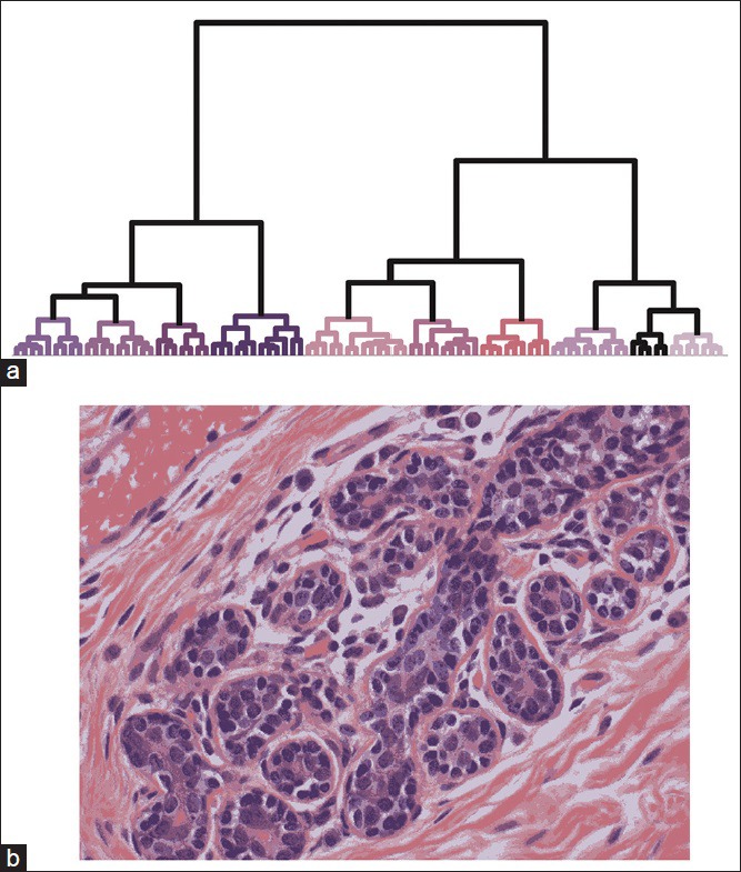
Color reduction for user characterization. (a) Hierarchical clustering of the pixels in Figure 2a produced 10 clusters, each represented by a different color in the dendrogram. Colors matched the cluster's centroid, except for lumen which is designated black for clarity. The heights of the connecting links in the dendrogram represent the dissimilarity between two clusters. For clarity, only the top of the dendrogram is shown and therefore nodes corresponding to single pixels are not visible. (b) A pseudocolor representation was formed by assigning each pixel to one of the clusters shown in (a)

We grouped pixels according to similarity in HSV space using an agglomerative hierarchical clustering algorithm that sought to minimize intracluster variance while maximizing the Euclidean distances between clusters. Clusters were serially merged according to this rubric until only 10 clusters remained, at which point the procedure was terminated. In Figure 2b, a dendrogram depicting the result of the clustering procedure is shown for the image from Figure 2. For visualization purposes, the color assigned to each of the 10 clusters in the lower dendrogram branches was determined by the color of the cluster centroid. The three major divisions in the dendrogram (four groups on the left, three groups in the middle, and three groups on the right) primarily correspond to nuclei, stroma, and white space, respectively. When the color of each pixel in the image was remapped to the centroid of the cluster to which it belonged, the resulting image retained most of the detail present in the original (compare Figures 1a–2b), even though it was composed of only 10 colors. This result demonstrates that the reduction to a tractable set of pixel values does not destroy the features of the image important for classification.

Figure 1.

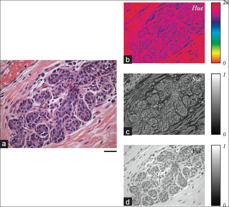
Hue, saturation, and value representation of a representative hematoxylin and eosin stained image. (a) A digital image of a normal breast lobular unit, showing distinct nuclear, cytoplasmic, and stromal regions. Scale bar: 50 μm. The hue (b), saturation (c), and value (d) components of the image shown in (a) are depicted

A pathologist in training was presented with the 10-color image and was asked to assign at least one color to the nucleus, cytoplasm, stroma, and lumen groups. Ambiguous colors were left unassigned. Typically, nuclei were comprised of one or two colors (mean: 1.34); cytoplasm one or two colors (mean: 1.57); stroma two, three, or four colors (mean: 2.86); and lumen one color (mean: 1.00). The pixels associated with the labeled colors served as the ground truth for the machine learning procedure, shown schematically in Figure 3. Pixels belonging to unassigned clusters were discarded from training. SVM learning was applied in a decision tree fashion to achieve multiclass classification. Lumen was first teased out from the image; nuclei were then extracted from the other tissue structures, and lastly, cytoplasm and stroma were distinguished from one another. This produced three SVM classifiers represented as planes in HSV space that optimally separated two sets of points from each other. In Figure 4, the classifiers for the case in Figures 1 and 2 are shown as dashed lines. To enable visualization of the planes in three-dimensional space, the data space was rotated so that the planes are directed out of the page. As expected, the planes appear to be optimally positioned to separate the different classes. The distributions of distances of pixels from the SVM hyperplanes are shown in the bottom panels of Figure 4. We used these distances, normalized by the distances separating the cluster centroids, as a measure of classification certainty.

Figure 3.

Support vector machine-based decision tree. A schematic of the machine learning procedure is illustrated, showing that unclassified data (open circles) can be classified in a serial fashion by sequentially applying binary support vector machine classifiers (denoted by the colored lines)

Figure 4.

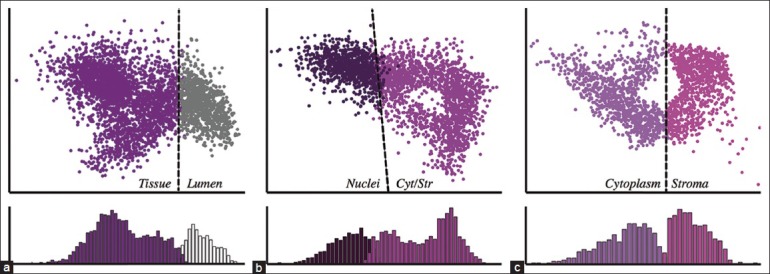
Support vector machine (SVM) classifiers derived from a single H&E stained image. SVM classifiers were computed from a ground truth supplied by the user in a serial fashion shown schematically in Figure 3. Hyperplanes are denoted by dashed lines. For clarity, data points are rotated in HSV space and projected into two dimensions so that the hyperplane extends out of the page. Histograms in the bottom panels represent the projection of points normal to the hyperplane and therefore represent the distribution of distances to the hyperplane. (a) Tissue versus lumen. (b) Nuclei versus cytoplasm and stroma. (c) Cytoplasm versus stroma

To demonstrate the classification capabilities of the algorithm, we applied the algorithm to 44 whole slide images of H&E stained slides, three of which are shown in Figure 5. For this figure, we selected images that appeared to be more difficult to classify or that contained structures that were not explicitly accounted for in the training. In the right panels, each pixel is depicted with a color according to the class to which it was assigned redundant and the intensity of the color was proportional to the distance of the pixel from the classification plane. Therefore, high intensities in the pseudocolor images were associated with more certain classifications, whereas low intensities indicated less certain predictions.

Figure 5.

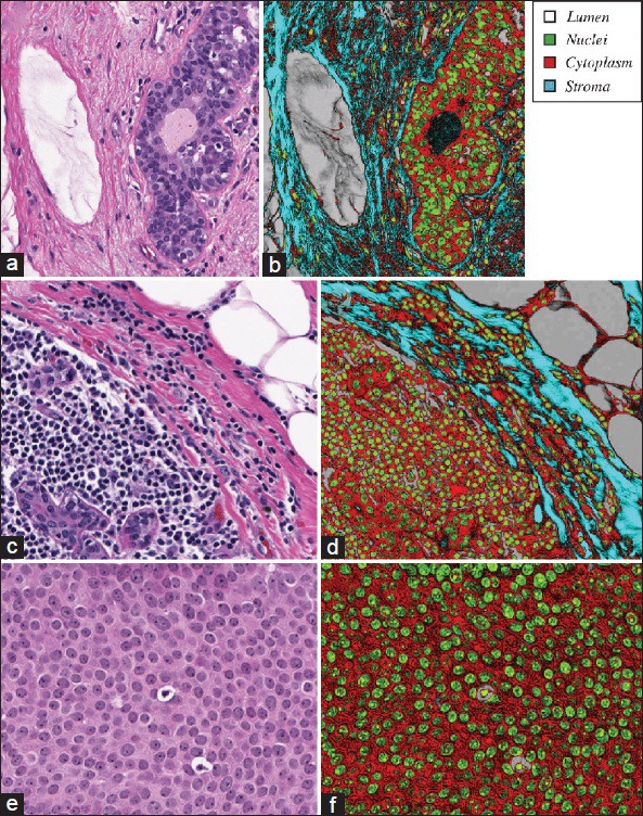
Classification maps. (a-b) Three representative images were selected at different scales and with different histological content (left panels). (c-d) Classification was performed to assign each pixel to one of four classes, and accompanied by a measure of confidence proportional to the normalized distance of a pixel from the classifying hyperplane. (e-f) In the right panels, the class is denoted by one of four pixel hues (legend) and confidence determined pixel intensity as described in methods

In Figure 5a–b, all four histologic structures are prominently represented. Dark bands pervade the image, indicating low classification confidence primarily associated with the stromal components surrounding the most cellular portion of the image. However, the majority of nuclei in the image are accurately defined and demarcated. An image such as this lends well to serving as the input to many established nuclear segmentation algorithms (data not shown). Notably, the fibrin in the lumen of a vessel (left) and the lumen in a gland (right) exhibit low classification accuracy. Retrospective analysis of this observation revealed that these colors were not included in the initial training step, and so the machine learning procedure was unable to classify them accordingly. Importantly, however, they were not incorrectly assigned to the most similar class (stroma); rather, the scalar nature of the output effectively flagged these regions as weakly classified.

Figure 5c–d exhibits similar classification performance and demonstrates that multiple cell types can be captured using a single nuclear classifier. Also apparent from this image is that the white space that we have nominally associated with lumen is also shared by fat. Distinguishing the two is beyond the scope of this paper and likely requires shape and contextual cues. However, those analyses, the plural of analysis could potentially benefit from this initial color mapping.

Figure 5e–f is shown at a different scale to demonstrate a case where less prominent nuclei in this image of DCIS solid type, low grade, can still be identified given a sensitive classifier. All or parts of most nuclei are identified in this figure, which can prove useful for operations such as cell counting. Furthermore, the scalar nature of the algorithm's output enables the identification of the prominent nucleoli, as they tend to exhibit very high classification certainty values. Likewise, two necrotic cells are evident in the image and are represented with high classification values. They are also surrounded by a halo of white space, which is correctly classified.

It is evident from the images in Figure 5 that some areas exhibit lower classification certainties than others. Generally, this was the case for pixels classified as nuclei and cytoplasm, whereas white space usually exhibited higher classification certainty [Figure 6]. Stroma exhibited an intermediate level of certainty, consistent with the observations in Figure 5 of both very strong and very weak bands. However, these trends are less obvious in the histograms shown for the normal breast case in Figure 4, in which the data points associated with the stroma and nuclei tended to aggregate more closely to their corresponding hyperplanes. It remains unclear whether the stromal features, in this case, could be considered an outlier or whether this property is characteristic of normal breast tissue specimens.

Figure 6.

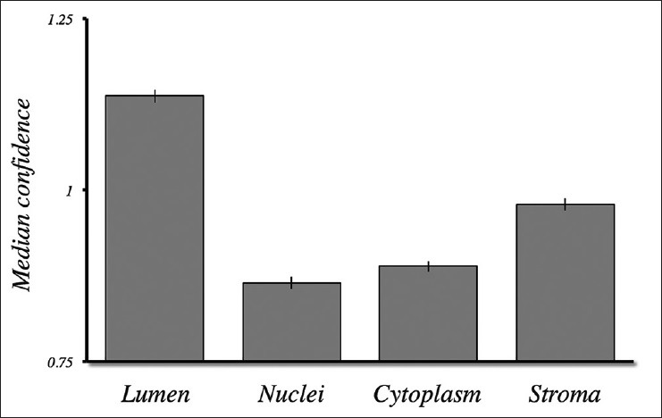
Classification confidence. The classification confidence, as the normalized distance from the classification hyperplane, was computed for 44 digital images from invasive breast carcinoma specimens. Lumen and stroma exhibited the highest median confidence values. Standard error bars are shown

Consistent with previous studies, we noted that there existed significant variation between samples prepared and stained by the same laboratory. By applying the classification procedure to 44 different images individually, we aimed to provide a quantitative account of these differences. We computed the centroids of each tissue structure in each of the 44 images, and although we confirmed that there was substantial variation, the centroids themselves exhibited very little overlap with centroids from other tissue structures [Figure 7a]. We noted, however, that the variation was anisotropic, especially for stroma. We measured the variation separately in the chromatic (hue-saturation) plane and intensity axis, and confirmed that the ratio of chromatic to intensity variability was much higher for stroma than for nuclei or cytoplasm [Figure 7b]. The result indicates that staining variation, which is similar in overall magnitude for the three tissue structures, mostly has a chromatic component for stroma, and, therefore, simple intensity adjustment is inadequate to correct for inter-specimen staining differences.

Figure 7.

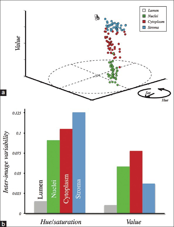
Inter-image variability. (a) Cluster centroids for each structure in each analyzed image are plotted in HSV space. Points representing lumen are also shown projected to the hue-saturation plane to demonstrate that they consistently congregate about (0, 0). (b) The variability across images was computed within the hue-saturation plane (left) and the value axis (right). Stroma varied most strongly in the hue-saturation plane relative to the other structures

We have demonstrated that images analyzed individually can be re-mapped into a new scalar space that may be used as a pre-processing stage for a number of functions, or may be used to characterize an image's consistency with other images (e.g., for calibration). This procedure, however, requires that a trained user first match the derived colors to their associated histological structures. We sought to determine whether this manual step could be eliminated after a sufficient number of training images were analyzed. We tested the classification performance of the algorithm using leave-one-out cross validation for our set of 44 images. We exploited the finding from Figure 7a that there is very little overlap between centroids associated with different histological structures. For each image, the centroids in HSV space of each cluster were compared to the centroids derived from the other 43 images. Those centroids that were sufficiently similar to the population of centroids were assigned to that structure in an automated fashion, replacing the manual classification stage in the computational pipeline. We evaluated the concordance rates between classified pixels based on automatic assignment and those based on manual assignment by A.P. We found that the median concordance rate was 0.95 for pixels that exhibited certainty levels >1 and 0.92 for pixels that exhibited certainty levels >0.5. The median proportion of pixels that exhibited certainty levels >1 and 0.5 was 0.56 and 0.79, respectively. Less certain classifications yielded slightly lower accuracy levels when compared to the manual procedure, but captured a greater proportion of pixels in the image. The ability to assign classification certainty values remains an important feature.

CONCLUSIONS

Evaluation of H&E stained specimens serves as the cornerstone for pathology diagnosis and staging. Here we demonstrate an algorithm that quantitatively characterizes the staining attributes of a sample and can identify tissue structures for the purpose of remapping to an alternate, optimized color space. Furthermore, we show that staining variability has a diverse signature for different tissue structures, further elucidating the difficulty in applying many popular approaches to image normalization metrics.

Remapping H&E digital images to an alternate color space supports a number of functions important for pathology. For instance, cell counting may be reliably performed; nuclear segmentation may be more accurately applied to support morphometric operations; substructures such as nucleoli may be identified and measured; nuclear-cytoplasmic ratio may be accurately computed; and structure identification may be accomplished to aid in diagnosis or ROI selection. In addition, research endeavors with clinical implications that rely on image processing could be standardized and become more reproducible. Furthermore, a quantitative account of staining attributes could be used for the purposes of daily laboratory quality control and calibration. These functions position digital pathology in a more active role in the pathology laboratory.

The technique that we report relies on user intervention to establish a ground truth necessary to train the machine learning algorithm. It may be desirable to remove this manual component in order to automate the procedure fully. Given the substantial inter-specimen variability that has been reported and that we confirmed, it is difficult to derive a single classifier that can directly be applied to all specimens while maintaining high classification accuracy, especially across laboratories. However, the insights gained from the results in Figure 7 provide a substrate on which models can be built for classification. The first stage of the algorithm is a data-driven unsupervised clustering procedure, and, therefore, produces initial groupings that are specific to the slide analyzed. In this way, the clustering step accounts for the inter-specimen variability. Since there was very little overlap in the tissue centroids across specimens, a classifier can be built from the results in Figure 7 to designate each cluster to a histologic structure in an automated fashion. The algorithm can then proceed to classify all pixels in the image based on the SVM decision tree framework. It is important that this initial training be performed on a representative set of cases from the laboratory or research data set. We showed that automation of this step did not drastically change the classification maps for those pixels that exhibited high classification certainty.

We arbitrarily chose to reduce ROIs initially to 10 clusters. A larger number of clusters may allow for less represented pixels to more accurately be characterized by the user, allowing them to be included in the training stage. However, more clusters may also lead to greater overlap between tissue structures, which may make an automated stage as described above more difficult to implement. This tradeoff needs to be explicitly tested to determine the optimum number of clusters to generate. Alternatively, a terminal condition could be specified that forces the hierarchical clustering procedure to terminate when specific criteria are met.

For demonstration purposes, we chose to classify four histologic structures in this report (nuclei, cytoplasm, stroma, white space associated with lumen), but the algorithm we describe has more general applicability. Specifically, it allows for a remapping of color space given an a priori set of structures, but this group can be augmented to accommodate other structures commonly found in other tissues or to subgroup nuclei, for instance, into different cell types. One such application may be the identification and quantification of inflammation in a sample.

Other clustering methods can potentially be used to perform tissue classification without the need for the SVM decision tree stage. In fact, some fuzzy clustering techniques could also produce scalar values that can be used as classification certainty measures. We believe the procedure described in this report has several advantages over a single-stage clustering algorithm for classification. First, two-stage algorithms do not require that the number of clusters matches the number of classes, allowing for these two variables to be manipulated independently for optimized performance. Second, the procedure we describe has a built-in mechanism for discarding ambiguous clusters from training while still being able to classify all pixels in the image. A second stage is necessary to incorporate the discarded pixels back into the classification schema. Third, SVM is most strongly influenced by data points closest to the putative classification boundaries (the support vectors). The two-stage model allows us to treat the data set initially according to cluster means for user evaluation, and then refine the classification based on an examination of the pixels at the cluster boundaries. Although this makes the algorithm sensitive to user error (e.g., by definitively assigning ambiguous clusters to tissue structures), it constructs classifiers based on the hardest-to-characterize pixels, which may improve classification of the ambiguous clusters that are more likely to reside near cluster boundaries. A cursory analysis of the pixels that served as support vectors for a subset of cases confirmed that they were indeed assigned to the correct structures (data not shown). Fourth, the scalar value produced by the SVM decision-tree is the projection of the vector orthogonal to the hyperplane that serves as the classifier. Importantly, SVM can construct hyperplanes in a non-linear fashion for improved classification accuracy. Although this was not performed here, this allows the orthogonal vector to position itself effectively in the data space non-linearly, allowing for non-Euclidean projections that may more accurately define classification certainty. This feature is difficult to accomplish with many other algorithms. Finally, since the first stage operates using relatively small samples, it is more computationally efficient than agglomerative clustering methods that require larger samples (or entire data sets). Divisive clustering methods that do not require point-by-point analysis could alternatively be used, but outlier detection with such methods often suffers, potentially increasing the number of ambiguous pixels incorporated into clusters. For these reasons, the SVM decision tree classification model is a robust tool for this application.

REFERENCES

- 1.Boiesen P, Bendahl PO, Anagnostaki L, Domanski H, Holm E, Idvall I, et al. Histologic grading in breast cancer – Reproducibility between seven pathologic departments. South Sweden Breast Cancer Group. Acta Oncol. 2000;39:41–5. doi: 10.1080/028418600430950. [DOI] [PubMed] [Google Scholar]
- 2.Dalton LW, Pinder SE, Elston CE, Ellis IO, Page DL, Dupont WD, et al. Histologic grading of breast cancer: Linkage of patient outcome with level of pathologist agreement. Mod Pathol. 2000;13:730–5. doi: 10.1038/modpathol.3880126. [DOI] [PubMed] [Google Scholar]
- 3.Gurcan MN, Boucheron LE, Can A, Madabhushi A, Rajpoot NM, Yener B. Histopathological image analysis: A review. IEEE Rev Biomed Eng. 2009;2:147–71. doi: 10.1109/RBME.2009.2034865. [DOI] [PMC free article] [PubMed] [Google Scholar]
- 4.Rabinovich A, Agarwal S, Laris C, Price JH, Belongie SJ. Unsupervised color decomposition of histologically stained tissue samples. Adv Neural Inf Process Syst. 2004;16:667–74. [Google Scholar]
- 5.Ruifrok AC, Johnston DA. Quantification of histochemical staining by color deconvolution. Anal Quant Cytol Histol. 2001;23:291–9. [PubMed] [Google Scholar]
- 6.Hang C, Loss LA, Spellman PT, Borowsky A, Parvin B. Biomedical Imaging (ISBI), 2012. 9th IEEE International Symposium on 2012; Batch-invariant nuclear segmentation in whole mount histology sections. [Google Scholar]
- 7.Latson L, Sebek B, Powell KA. Automated cell nuclear segmentation in color images of hematoxylin and eosin-stained breast biopsy. Anal Quant Cytol Histol. 2003;25:321–31. [PubMed] [Google Scholar]
- 8.Vidal J, Bueno G, Galeotti J, García-Rojo M, Relea F, Déniz O. A fully automated approach to prostate biopsy segmentation based on level-set and mean filtering. J Pathol Inform. 2011;2:S5. doi: 10.4103/2153-3539.92032. [DOI] [PMC free article] [PubMed] [Google Scholar]
- 9.Isitor GN, Thorne R. Comparison between nuclear chromatin patterns of digitalized images of cells of the mammalian testicular and renal tissues: An imaging segmentation study. Comput Med Imaging Graph. 2007;31:63–70. doi: 10.1016/j.compmedimag.2006.10.005. [DOI] [PubMed] [Google Scholar]
- 10.Ballarò B, Florena AM, Franco V, Tegolo D, Tripodo C, Valenti C. An automated image analysis methodology for classifying megakaryocytes in chronic myeloproliferative disorders. Med Image Anal. 2008;12:703–12. doi: 10.1016/j.media.2008.04.001. [DOI] [PubMed] [Google Scholar]
- 11.Kayser K, Görtler J, Metze K, Goldmann T, Vollmer E, Mireskandari M, et al. How to measure image quality in tissue-based diagnosis (diagnostic surgical pathology) Diagn Pathol. 2008;3(Suppl 1):S11. doi: 10.1186/1746-1596-3-S1-S11. [DOI] [PMC free article] [PubMed] [Google Scholar]
- 12.Wittekind D. Traditional staining for routine diagnostic pathology including the role of tannic acid 1. Value and limitations of the hematoxylin-eosin stain. Biotech Histochem. 2003;78:261–70. doi: 10.1080/10520290310001633725. [DOI] [PubMed] [Google Scholar]
- 13.Ward JH. Hierarchical grouping to optimize an objective function. J Am Stat Assoc. 1963;58:236–44. [Google Scholar]
- 14.Vapnik VN. An overview of statistical learning theory. IEEE Trans Neural Netw. 1999;10:988–99. doi: 10.1109/72.788640. [DOI] [PubMed] [Google Scholar]