Automated image based prominent nucleoli detection

Abstract

Introduction:

Nucleolar changes in cancer cells are one of the cytologic features important to the tumor pathologist in cancer assessments of tissue biopsies. However, inter-observer variability and the manual approach to this work hamper the accuracy of the assessment by pathologists. In this paper, we propose a computational method for prominent nucleoli pattern detection.

Materials and Methods:

Thirty-five hematoxylin and eosin stained images were acquired from prostate cancer, breast cancer, renal clear cell cancer and renal papillary cell cancer tissues. Prostate cancer images were used for the development of a computer-based automated prominent nucleoli pattern detector built on a cascade farm. An ensemble of approximately 1000 cascades was constructed by permuting different combinations of classifiers such as support vector machines, eXclusive component analysis, boosting, and logistic regression. The output of cascades was then combined using the RankBoost algorithm. The output of our prominent nucleoli pattern detector is a ranked set of detected image patches of patterns of prominent nucleoli.

Results:

The mean number of detected prominent nucleoli patterns in the top 100 ranked detected objects was 58 in the prostate cancer dataset, 68 in the breast cancer dataset, 86 in the renal clear cell cancer dataset, and 76 in the renal papillary cell cancer dataset. The proposed cascade farm performs twice as good as the use of a single cascade proposed in the seminal paper by Viola and Jones. For comparison, a naive algorithm that randomly chooses a pixel as a nucleoli pattern would detect five correct patterns in the first 100 ranked objects.

Conclusions:

Detection of sparse nucleoli patterns in a large background of highly variable tissue patterns is a difficult challenge our method has overcome. This study developed an accurate prominent nucleoli pattern detector with the potential to be used in the clinical settings.

INTRODUCTION

Digital pathology has benefited from the development and assimilation of computer vision, machine learning, graphics as well as computing hardware technologies. Adaptation of informatics into clinical practices can be used to solve many key issues of pathology. Often, patients undergo needle biopsies of cancerous lesions to obtain accurate diagnosis. Due to inter-observer variability, even when assessed by experienced urologic pathologists, agreement in prostate cancer Gleason grading in 38 of 46 cases, for instance, could be as low as 70%.[1] In laboratories with differences in individual pathologist training and the small amount of tissue samples obtained from needle biopsies, accuracy in diagnosis and detection of these lesions may be even more difficult.[2] The cytologic features that indicate cancerous tissue are nuclear enlargement, hyperchromasia, and prominent nucleoli. A pathologist must differentiate these to give accurate stratification of risks in prostate cancer using the Gleason grading system. For renal cancers, there are several cell types that affect treatment and prognosis. The ability to differentiate clear cell renal cancer from papillary cell renal cancer (either Type 1 or Type 2) will change the prognosis and management of individual patients. The molecular profiles and targeted therapy in these different cell types of renal cancers are vastly different.

The analysis of prominent nucleoli is one of the several important considerations for cancer prognosis and diagnosis. Nucleolar features have been reported to provide an independent prognostic variable in 24 types of cancer.[3] For example, a study on breast cancer showed a significant difference in survival rates between two groups of patients separated by nucleolar size alone.[4] Prominent nucleoli patterns, an important parameter for the pathologist, are not sufficient to be the determining factor for cancer diagnosis.[3,5,6] Nevertheless, nucleolar size plays a central role in cell proliferation, and its morphology is closely related to cancer growth. It has been shown with high statistical significance that nucleolar size is proportional to cancer cell proliferation.[7,8] Prominent nucleoli number also increases with Gleason grading in prostate cancer.[9]

The nucleolus is the organelle where ribosome biogenesis occurs; increased ribosome production is required for proliferating cells. This process is tightly regulated in normal cells, but in cancer cells, such regulation may be perturbed giving rise to uncontrolled cell proliferation.[5] Hence, nucleolus morphology, ribosome biogenesis, and cancer are closely related.

In our study, we aimed to create an intelligent computational system that can learn and improve on its diagnosis of cancerous lesions through accurate detection of prominent nucleoli patterns. This system will assist the pathologist by highlighting prominent nucleoli patterns for more detailed analysis. It will serve as an additional tool that is objective, self-learning, non-fatigable, and has the ability to analyze individual single nucleolus in high power whole slide images thereby providing a report of suspicious areas in needle biopsy specimens.

RELATED WORK

The diagnosis of prostate cancer is based on a constellation of features rather than on any one criterion wherein architectural, nuclear, cytoplasmic, and luminal features are evaluated.[10] Prominent nucleoli are one of the criteria that indicates the diagnosis of prostate adenocarcinoma.[11,12,13]

For cancer in general, changes in the structure of the nucleus have long been recognized as diagnostically significant. These include increased nuclear size, deformities in nuclear shape, and changes in the organization of the nucleus to the extent that they are observable by light microscopy.[14,15,16] Although the diagnosis of prostate cancer is typically based on a combination of findings, the presence of prominent nucleoli is considered as one of the most influential factors diagnostically. In a recent study, Varma et al.[13] reported that prominent nucleoli were seen in 94% of cancers diagnosed on routine biopsy material. However, Epstein[11] observed only 76% of cases with nucleolar prominence in consultation-based needle biopsy material. There have been several studies that have examined nucleolar features in greater depth.[3,4,5,6,7,8,9]

The number and location of nucleoli have also been implicated as useful aids in the diagnosis of prostate cancer. Helpap[16] studied 300 prostate cancers of varying grades, 20 normal prostates, 10 cases of granulomatous prostatitis, and 40 cases of benign prostatic hyperplasia (BPH) removed by transurethral resection or fine-needle aspiration. In normal, granulomatous prostatitis and well-differentiated carcinoma, only one nucleolus was visible using dry and oil immersion lenses at magnifications of ×63 or ×100. Multiple nucleoli increased in frequency, paralleling the increase in tumor grade. However, even in the most poorly differentiated cancer of the nuclei with nucleoli, 87.4% had only one visible nucleolus. Normal prostate and prostatitis had only centrally located nucleoli, and peripherally located nucleoli was noted in 14% and 49% of the nuclei within well and poorly differentiated cancers, respectively.

Despite advances in the morphological diagnosis of prostate cancer and the contribution of immunohistochemistry, there remains a group of cases where diagnosis remains uncertain. This study sought to analyze whether nucleoli detection through high-resolution computational methods can serve as a detection support system in prostatic adenocarcinoma. The project will provide seminal work in the analysis of digitized tissue sections. Furthermore, the assessment of nucleoli in digital images will represent an initial step toward influencing future developments such as the analysis of other features of carcinomas like architectural patterns in prostate tumors.

The emergence of digital pathology gave rise to many computational methods modeled on popular pathological grading systems such as the Nottingham, Gleason, and Fuhrman grading systems.[17,18,19] These computational methods were developed in a framework suitable for implementation of machine learning. Machine learning methods such as support vector machines (SVMs), Bayesian classifiers, AdaBoost, and shape manifold learning are used for classification purposes.[20,21,22,23,24] Additionally, low-level image analysis such as image segmentation and image feature extraction are also required to achieve good results. The main types of image features used are morphological, textural, fractal, topological, and intensity-based features. A major challenge of automated diagnosis is finding the best subset of image features.[17]

As suggested in the Gleason grading system, methods in the literature use gland morphology to distinguish between grades of prostate cancer.[21,22,25,26,27] Inspired by the procedure generally adopted by pathologists, a cancer detection system was proposed utilizing cytological and textural features.[28,29]

Different texture-based methods have been reported in the literature.[25,26,30,31] A texture-based classification system for the Gleason grading used random forests to cluster the response of various filters.[31] In another study, texture features along with morphological features were used to identify stroma, normal, and cancerous regions in prostate histopathological images.[26]

To speed up the computation of image features, a Field-Programmable Gate Array was programmed for Haralick texture feature extraction.[32,33] Principal component analysis (PCA) has been used to reduce the feature dimensions for classification of architecturally differentiated images of prostate cancer.[34] A framework for learning shape manifolds for various nuclei shapes with PCA was developed to reduce computational complexity.[23,35] Following a signal processing approach, the histopathological images (signals) can be expressed as a linear combination of basis vectors (signals) using sparse coding. Whole slide image analysis has been done in an efficient way using sparse coding with dynamic sampling.[36] Observing that the intrinsic pattern of cancer tissue is self-similar such as fractals, some methods using fractal dimensions have also been proposed.[37,38] Energy, entropy, similarity measurement methods, fuzzy spatial clustering, and level set contours have been used for feature extraction of prostate histopathological images.[34,39,40] Cardinal multiridglet transform has also been employed to classify prostate images into Gleason grades 3 and 4.[41] A multi-spectral method using 16 spectral bands instead of grayscale or RGB images was used to classify tissue image blocks into stroma, BPH, prostatic intraepithelial neoplasia, and different grades of prostate cancer.[42]

Many computational methods for breast cancer detection focus on mitotic count. A multi resolution approach was used for grading breast cancer to detect and classify individual cells utilizing all criteria of the Nottingham grading system.[43] Utilizing an alternative method, deep neural networks were used to classify pixels as mitosis and non-mitosis.[44]

DATASETS

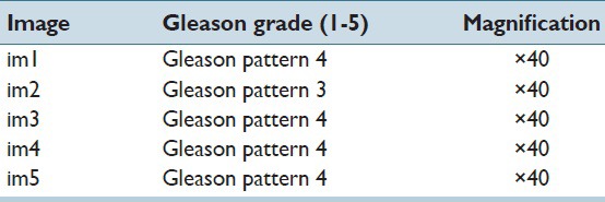
Hematoxylin and eosin (H&E) stained images of the prostate, breast, renal clear cell, and renal papillary cell cancers were used to demonstrate the effectiveness of our proposed method. The first dataset consisted of four images of Gleason pattern 4 and one image of Gleason pattern 3, each sized at 1360 × 1024 pixels. This set of data was carefully selected by a trained pathologist to develop the program. The other datasets consisted of 12 1360 × 1024 pixels images of infiltrating ductal carcinoma, nine 1360 × 1024 pixels images of renal clear cell carcinoma, and nine 2720 × 2048 pixels images of renal papillary carcinoma. These data were extracted from a public repository hosted by The Cancer Genome Atlas (TCGA) (https://tcga-data.nci.nih.gov/tcga), and utilized for validation and testing purposes of the nucleoli detection program. We give details of the TCGA datasets in the Tables 1–3. The top left corner of the digital slide is used as the origin of the X-Y coordinate system. In the images, the X-axis is horizontal and Y-axis vertical. Table 4 describes the prostate cancer dataset images. All the images were at ×40.

Table 2.

Images cropped from TCGA renal clear cell cancer data

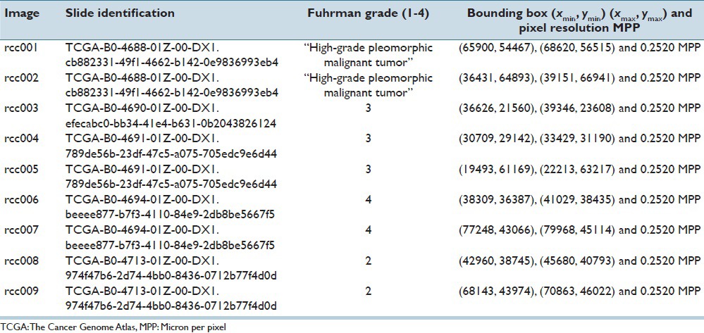
Table 1.

Images cropped from TCGA breast cancer data

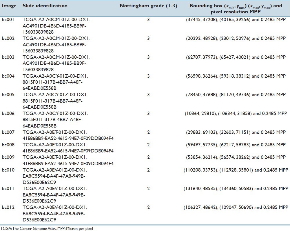
Table 3.

Images cropped from TCGA renal papillary cell cancer data

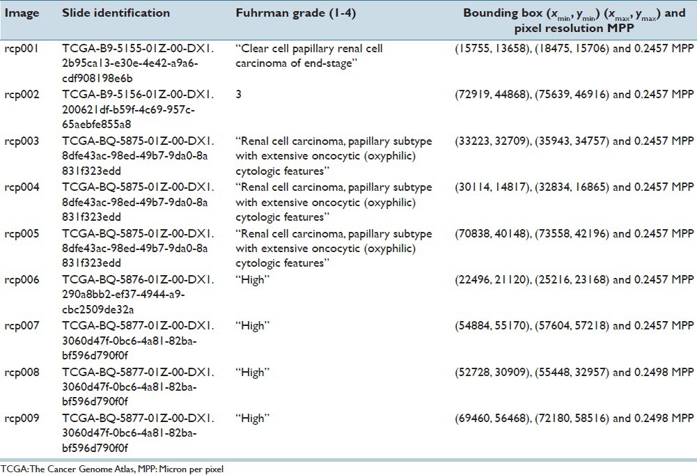
Table 4.

Images obtained from transrectal ultrasound guided biopsy of patients with prostate cancer

DESCRIPTION OF PROSTATE CANCER DATASET

Paraffin-embedded archival tissues of a local Asian population were obtained from our laboratory. Prostatic tissues were acquired from patients who underwent transrectal ultrasound guided prostate biopsy. The slides were carefully selected to contain representative patterns of prominent nucleoli. The Olympus BX 51 microscope and Olympus DP 71 camera were used to capture the images at ×40 objective magnification.

Two important features within the images that were identified are: Gland morphology and the existence of prominent nucleoli. Fifty regions that exhibited both of these features were manually extracted. As the main purpose of this project was nucleoli detection, we placed emphasis on nucleoli visibility. Thus, five of the images that contained a total of 778 prominent nucleoli deemed to satisfy this criterion were selected.

DESCRIPTION OF BREAST, RENAL CLEAR CELL AND RENAL PAPILLARY CELL CANCER DATASETS

Four whole slide images of breast cancer with Nottingham grading of 2 and 3 (two images each) were downloaded from the TCGA website. Three images of size 2720 × 2048 pixels from each slide were cropped out and down-sized to 1360 × 1024 pixels and 3753 nuclei with a prominent nucleolus were manually annotated.

Five whole slide images of renal clear cell cancer were downloaded. One slide was marked as Fuhrman grade 2, two slides as Fuhrman grade 3, one slide as Fuhrman grade 4, and the last slide as “high-grade pleomorphic malignant tumor”. Nine images sized 2720 × 2048 pixels were cropped out and downsized to 1360 × 1024 pixels and 2072 nuclei with a prominent nucleolus were manually annotated.

Five whole slide images of renal papillary cell cancer were downloaded. One slide was marked as Fuhrman grade 3, two slides as ‘high grade cancer’, one slide as ‘clear cell papillary renal cell carcinoma of end-stage kidney’, and the last slide as ‘renal cell carcinoma, papillary subtype with extensive oncocyte (oxyphilic) cytologic features’. Nine images of size 2720 × 2048 pixels were extracted, and 2919 nuclei with prominent nucleolus were annotated.

COLOR SPACES CONVERSIONS

All images were acquired or downloaded as three-channel images in the RGB representation. Duplicates were made of the images and converted into different color spaces, RGB, HSV, HLS, XYZ, CIELAB, CIELUV, and YCbCr. Processing the data in different color spaces emphasizes different aspects of the prominent nucleoli patterns.

Throughout this paper, we processed the data with different color spaces independently. Only in the final step of our algorithm were the results of different color spaces combined using the RankBoost algorithm.[45]

METHOD

Overview

An object detector, trained on an ensemble of cascades, is used to detect the patterns of prominent nucleoli in large regions of whole slide images. Each cascade is similar to the cascade of classifiers proposed by Viola and Jones.[46] The image features of each pixel are derived from a variable image patch of size s × s pixels centered at that pixel. Individual pixels in the dataset are either predicted by a cascade as negative, in which case no score is given to that pixel, or predicted as positive in which case a score is assigned proportional to the likelihood of this pixel representing an image patch containing the pattern of prominent nucleoli.

The output of each cascade is used to rank, in descending orders of the score, all predicted positive pixels, generating an ensemble of ranks. The RankBoost algorithm is used to combine this ensemble of pixel level ranks. For each test image, every pixel is either labeled negative or ranked in accordance to its likelihood of representing the pattern of prominent nucleoli. The final pixel level ranking derived from RankBoost is then converted into object level ranking. Finally, we present the image patch object to the pathologist for validation in the order of its object level ranking.

Effective ranking of detected objects can reduce the manual work of the pathologist significantly because our software can present the most relevant information to the pathologist without the need to manually scan through large areas of the image slides.

The Cascade Detector

A cascade is constructed by stacking 20 classifiers sequentially. The top classifier is trained on the input data while subsequent classifiers are trained using the output of classifiers directly above it. A detailed description of the cascade can be found in Viola and Jones.[46] A simple image filter is used namely, the “Find Maxima…” function of ImageJ,[47,48] followed by image dilation with a 9×9 square window which is added to filter out obvious negatives at the top of the cascade. Four classification methods are used to populate the layers of cascades – histogram of polar gradient (HPG), enhanced histogram of polar gradient (EHPG), eXclusive Component Analysis (XCA) and logistic regression (LR). The HPG and EHPG classifiers are specially designed to extract prominent nucleoli patterns. XCA has been shown to be effective for a similar dataset.[49] LR was chosen as a “baseline” classifier to be compared to the more sophisticated HPG, EHPG, and XCA classifiers.

Permuting different combinations of classifiers generates cascades of different configurations to form an ensemble of cascades. Each cascade assigns a score to predicted positive pixels. These scores are subsequently used in a ranking algorithm that is described in Section “Ensemble of Cascades”.

Histogram of Polar Gradient

For each pixel, we extract an image patch of s × s pixels. A polar gradient histogram is extracted from this image patch and used as the feature of the pixel. Following which, a SVM is trained using HPG features on the labeled image patches.

Histogram of the polar gradient is a variant of the histogram of gradient (HOG) method.[50] Instead of the gradient information used in HOG, HPG computes the image gradient in polar coordinates, u_r (x, y) and u_θ (x, y) let be a three channel image.

where and are the radial and angular unit vectors of pixel (x, y) with respect to the center of the image patch. Next we extract the channel with the maximum response to the gradient operator,

This representation captures the features of most prominent nucleoli which are round in shape. HPG uses the same 3 × 3 block structure as in HOG, but the histogram is constructed in a slightly different manner.

Let ∂U denote the space of possible values of u_r, u_θ and B = {1,…,9} denote the set of blocks. A rectangular window w_i ⊂ ∂U × B can be defined by, w_i = (u^min_r, u^max_r, u^min_θ, u^max_θ, b) u^min_r, u^max_r, u^min_θ, u^max_θ define a bounding box in ∂U and b ∈ B specifies from which block the image gradient is calculated from. Each pixel in the s × s image patch generates a triplet of number (u_r, u_θ, b). (In the case when s is odd, s × s − 1 triplets of (u_r, u_θ, b) are generated, gradient information of the center pixel is discarded where the polar gradient is not well defined.) u_r and u_θ are defined in Eq. (2) and b is the block number in which this pixel belongs to [Figure 1]. A histogram count h_i can be generated by counting the number of points (u_r, u_θ, b) that fall within the window w_i. A scatter plot of u_r, u_θ, b is used to obtain a representative set of image patches containing prominent nucleoli (positive image patches) and background (negative image patches). From the pattern of the scatter plot, 31 rectangular windows w_i are manually selected that is discriminative for the classification of positive and negative image patches. Figure 1 shows how the image patch is compartmentalized and how the histogram counts are generated. Finally, these 31 features are fed into the radial basis function (RBF) kernel SVM to build our classifier. Tuning of SVM parameters is discussed in Section “RESULTS”.

Figure 1.

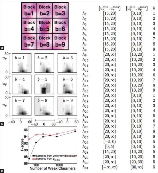
(a) How the s × s pixels image patch is divided into blocks. (b) The plot of p_EHPG (u_r, u_θ, b) for each block. x-axis represents u_r and y-axis represents u_θ. Dark areas represent areas of high probabilities. Notice that windows around u_r ≈ 0 and u_θ ≈0 at block b = 5 are sampled at high frequency. (c) That F-score for classification increases with the use of p_EHPG for sampling windows w_i. The right table shows the ranges of u_r, u_θ and b values in which histogram counts are accumulated for HPG features

Enhanced Histogram of Polar Gradient

In the EHPG, an ensemble of random rectangular windows is generated instead of manually selecting rectangular windows for the histogram counts as in HPG. Their histogram counts are used as the feature. One weak classifier is constructed for each histogram count. The AdaBoost[51] algorithm is then used to combine the ensemble of weak classifiers to form a strong classifier. The weak classifier c_i is constructed as follows. First a random point in the space of ∂U × B is sampled from a distribution (u_r,i, u_θ,_i, b_i) ∼ p_EHPG (u_r, u_θ, b) and then a rectangular window w_i is sampled with u_{r, i}, u_{θ, i} being the center of the window. Width and height of the window are sampled independently and uniformly from the range 4 to 10 units of u_r, u_θ. The training data is used to tune the sizes of windows so that the performance of the weak classifiers is optimized. The distribution p_EHPG (u_r, u_θ, b) is constructed using our training data. The weak classifier is given by,

h_i is the number of gradient points that fall within w_i,τ_i is a threshold value and π_i = ±1 is a parity variable. The values of τ_i and π_i are adjusted to optimize the weak classifier using the training dataset. The AdaBoost algorithm is then used to combine the weak classifiers,

α_i are the weights assigned by AdaBoost.

For the construction of p_EHPG, a large number of random windows w_i are sampled uniformly from the u_r, u_θ and b space. Weak classifiers are constructed, and AdaBoost is used to determine the weights, α_i. Each point in (u_r, u_θ, b) ∈ ∂U × B may be covered by multiple windows w_i and each window is associated with an AdaBoost weight α_i. An importance score for each point (u_r, u_θ, b) is assigned by summing the AdaBoost weights associated with all windows w_i that cover the point. The scores overall points (u_r, u_θ, b) are then normalized to obtain p_EHPG (u_r, u_θ, b). Figure 1 shows that using p_EHPG improves the classification results.

eXclusive Component Analysis

A labeled set of image patches can be partitioned into positive and negative subsets of image patches. XCA[49] identifies three kinds of patterns–patterns of the image patches that are common to both positive and negative subsets, patterns that are exclusive to the positive subset and patterns that are exclusive to the negative subset. These common and exclusive patterns are encoded in the form of basis functions for the image patches, such that each image patch is a linear combination of the basis functions. Detailed theory and implementation for mitosis detection in breast cancer images are described in Huang et al.[49]

Logistic Regression

We use standard LR and the gradient descent method to find our parameters. To reduce the number of parameters, we convert the three channel image patch into one channel using the formula, u_LR (x, y) =1/3 [u₁ (x, y) + u₂ (x, y) + u₃ (x, y)], and use the raw pixel values of u_LR (x, y) for an image patch of s × s pixels as the input of the LR.

Ensemble of Cascades

Twenty levels of classifiers were used for all our cascades. By permuting different combinations of four classifiers, a large number of classifier configurations can be generated. For each classifier configuration, we train the cascade on seven different color spaces and on different scales (n_scales image patch sizes).

7n_scales × 4²⁰ possible cascades can be generated. In our experiments, we use several hundreds of cascades for each test image. Each cascade will generate a score for predicted positive pixels. Let X_i, i = 1,…, n be the set of pixels that are predicted positive for the i^th cascade, where n is the total number of cascades, including cascades with different classifier configuration on different color spaces and scales. A ranking order R_i can then be assigned to X_i by sorting according to the score in descending order. We can generate a set of pixels U = Uⁿ_i=1X_i that contains all pixels that are predicted positive by at least one cascade. The RankBoost[45] algorithm is then used to combine all ranking order R_i, i = 1,…, n generating a better rank order R_U on the set U.

From Pixel Level to Object Level

Generally, a small cluster of pixels will be predicted to be positive if they are in the vicinity of a prominent nucleolus. However, all pixels in this small cluster really refer to a single object of the prominent nucleolus. As described in Section “Ensemble of Cascades”, all predicted positive pixels are converted to a rank order R_U using the RankBoost algorithm. To extract objects out of pixel-level detection, the highest ranked pixel will be assigned to represent one object within an image patch of s × s pixels. All other predicted positive pixels within an overlap ratio from this pixel are removed. The overlap ratio between two pixels associated with two image patches w_i and w_j, of given size s × s is defined as the area of overlap between w_i and w_j divided by the area of union of the two image patches,

The remaining predicted positive pixels are then re-ranked, and this process is repeated until no predicted positive pixels are left. Finally, a rank list of pattern of prominent nucleolus objects is generated.

RESULTS

Different image patch sizes were used for various datasets. For the HPG classifier, the libsvm RBF ν-SVM classifier was used and the libsvm parameters C and γ were set to 2 and 4 respectively. These values were tuned to optimize prediction accuracy using the prostate cancer dataset. The number of weak classifiers used for the EHPG classifier was set to 500 unless otherwise specified.

Figure 1c shows that the testing F-score increases with the number of weak classifiers used. However, computational efforts also increase with the number of weak classifiers. From the plot in Figure 1c, we chose to use between 150 and 500 weak classifiers to balance between having a good F-score and available computing resources. To reduce the computational complexity of XCA, dimensions of the image patch data were reduced to 16 principle components to balance between prediction accuracy and computational efficiency. We used a complete set of 16 basis unless otherwise specified. We have also performed experiments with under-complete basis sets. For the training of RankBoost, the unified set of pixels to be ranked U = Uⁿ_i=1X_i was divided into two disjoint subsets U₀ and U₁. All pixels having an overlap ratio of η ≥0.4 on a 24 × 24 pixel window (Eq. 5) with a labeled positive pixel belonged to U₁ and the remaining pixels to U₀. In this sense, all pixels in U₁ are those “in the vicinity of” prominent nucleoli pattern. A window size of 24 × 24 was used because this is approximately the size of a nucleus. An overlap ratio of 0.4 was used because pixels within this vicinity are clearly identified by the pathologist as the proximity of prominent nucleoli. We used 0.99 positive pattern retention rates for our cascades unless specified otherwise.[46] The method used for tuning this parameter is discussed in Viola and Jones.[46] We consider each detected object as a correctly identified pattern of prominent nucleoli if the pixel associated with this object was within an overlap ratio η ≥0.4 on a 24 × 24 image patch to a labeled prominent nucleoli pixel.

Cumulated Count and Major Challenges

A sparse distribution of prominent nucleoli patterns in a sizeable background of highly variable patterns makes it extremely challenging for object detection. In the prostate dataset, there were only 778 prominent nucleoli patterns in 6.9 million pixels. Hence, the object detector has to be very efficient even to detect a small fraction of prominent nucleoli patterns. Our object detector detected 58 prominent nucleoli in its first 100 ranked objects and missed 0.24% of the total number of prominent nucleoli patterns. In comparison, Figure 2 shows that using the method proposed by Viola and Jones[46] would perform about half as well. A detailed description of this comparison is given in Section “Effects of Using Different Number of Cascades and Different Combinations of Classifiers”.

Figure 2.

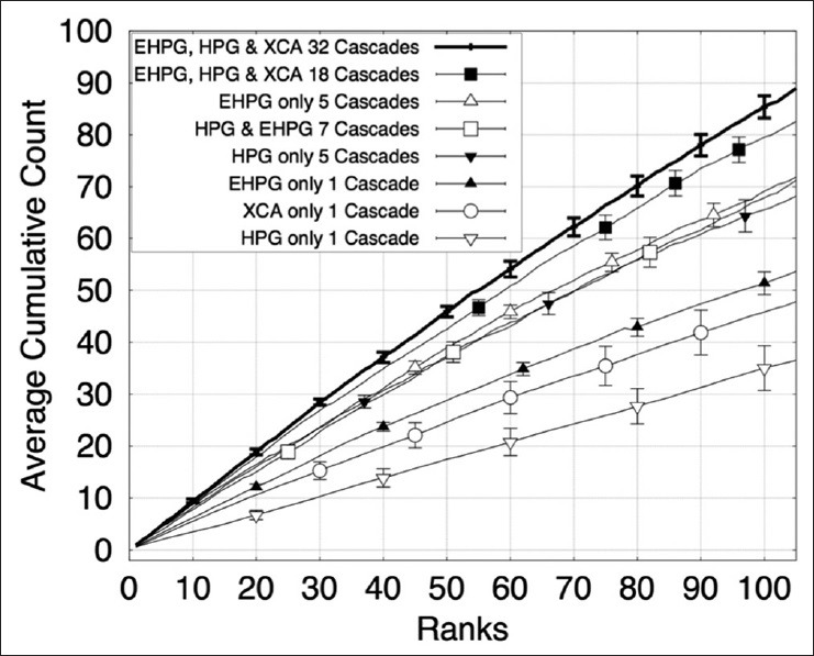
The plot shows the cumulative counts averaged over nine images versus ranks for prominent nucleoli patterns detected in the renal clear cell cancer dataset with error bars representing the standard error of the mean. We compared our result using different classifier combinations in our cascade and different numbers of cascades. HPG: Histogram of Polar Gradient classifier. EHPG: Extended Histogram of Polar Gradient classifier. XCA: eXclusive component analysis classifier

The cumulated count was used as a measure of the effectiveness of our algorithm. It is the cumulative number of objects detected correctly with respect to rank. For example, the cumulative count at rank = 20 is 18 which means that among the highest ranked 20 objects, 18 of these objects are detected correctly as prominent nucleoli pattern. The design of cumulated count is “pathologist centric”. Our software is most useful to the pathologist if it can present information in order of its relevance. Traditional measures of performance such as true positive rate may appear less useful for the pathologist.

Prostate Cancer Dataset

There were five images in this dataset; we performed five-fold cross validation, training on four images and testing on the remaining image. The image patch size used in this dataset was s × s = 24 × 24. This image patch size covers the pattern of prominent nucleoli well and is not large enough to include too much irrelevant background information. Classifiers used in the cascade were HPG, EHPG, XCA, and LR. In the XCA classifier, the number of basis functions used were 2, 4, 8, and 16. Figure 3 shows the average cumulated count versus ranks for the testing dataset. On average, our algorithm correctly detected 58 prominent nucleoli patterns in the top 100 ranked detected objects. Figure 4 shows that the top ten ranked image patches generated by our method accurately detects patterns of prominent nucleoli. The number of cascades for Image 1 was 288, Image 2 was 206, Image 3 was 220, Image 4 was 238, and Image 5 was 218. Although the cumulative count measure is better in terms of software usefulness to the pathologist, we report that the false negative rate was 0.24% ± 0.24%.

Figure 3.

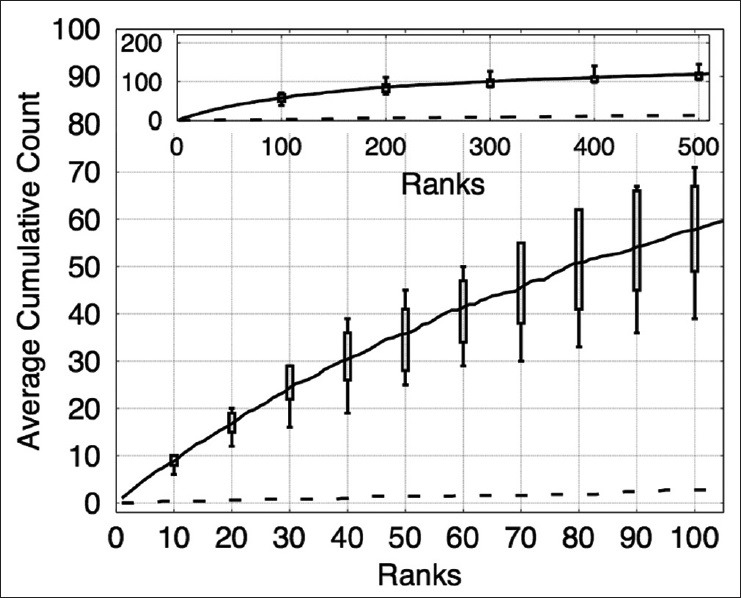
The plot shows the cumulative counts averaged over five images versus ranks for prominent nucleoli patterns detected in the prostate cancer dataset. The result for an algorithm that randomly ranks the pixels (dashed line) would fare much worse detecting only about 1.8% correct prominent nucleoli on average among its top 100 objects. The inset figure shows the average cumulative count curve for 500 ranked objects. The box plots indicate the first and third quarters of the data distribution. Horizontal bars show the highest and lowest cumulative counts

Figure 4.

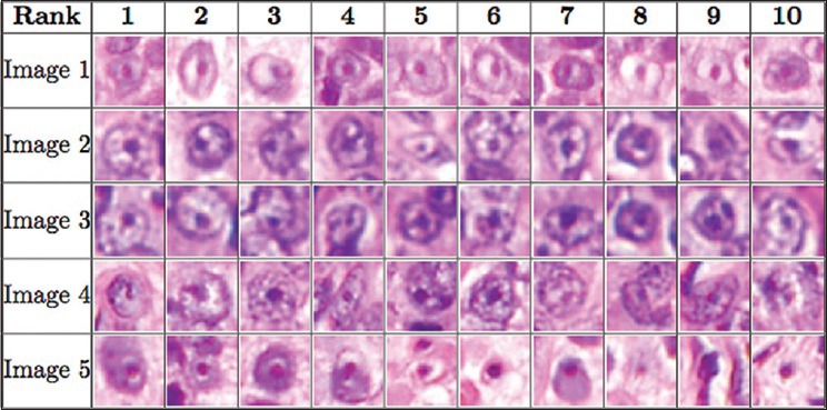
The figure shows the order of the ten most prominent nucleoli patterns to be presented to the pathologist for the prostate cancer dataset

Breast Cancer Dataset

There were 12 images in this dataset; we performed 12-fold cross validation, training on 11 images and testing on the remaining image. The image patch sizes used in this dataset were s × s = 15 × 15, 18 × 18, 21 × 21, 24 × 24, 27 × 27, and 30 × 30. Six different image patch sizes were used in order to combine the performance of our algorithm on different image resolutions. Classifiers used in the cascade were HPG, EHPG, and XCA. LR was found to be both computationally demanding and low in detection performance in the prostate dataset. It was therefore not used for the breast cancer dataset. For the EHPG classifiers, a mixture of EHPG with 150 and 500 weak classifiers were used in our cascades. Figure 5 shows the average cumulated count versus ranks for the testing dataset. On average, our algorithm correctly detected 68 prominent nucleoli patterns in the top 100 ranked detected objects. Figure 6 shows that the top ten ranked image patches generated by our method accurately detects patterns of prominent nucleoli. The number of cascades for Image 1 was 151, Images 2, 3, and 4 was 150, Image 5 and 6 was 149, Image 7 was 149, Image 8 was 144, Image 9 was 146, Image 10 was 148, Image 11 was 147, and Image 12 was 148. Our method missed 4.79 ± 4.67% of the total number of prominent nucleoli patterns.

Figure 5.

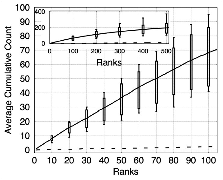
The plot shows the cumulative counts averaged over 12 images versus ranks for prominent nucleoli patterns detected in the breast cancer dataset. The result for an algorithm that randomly ranks the pixels (dashed line) would fare much worse detecting only about 5.3% correct prominent nucleoli on average among its top 100 objects. The inset figure shows the average cumulative count curve for 500 ranked objects. The box plots indicate the first and third quarters of the data distribution. Horizontal bars show the highest and lowest cumulative counts

Figure 6.

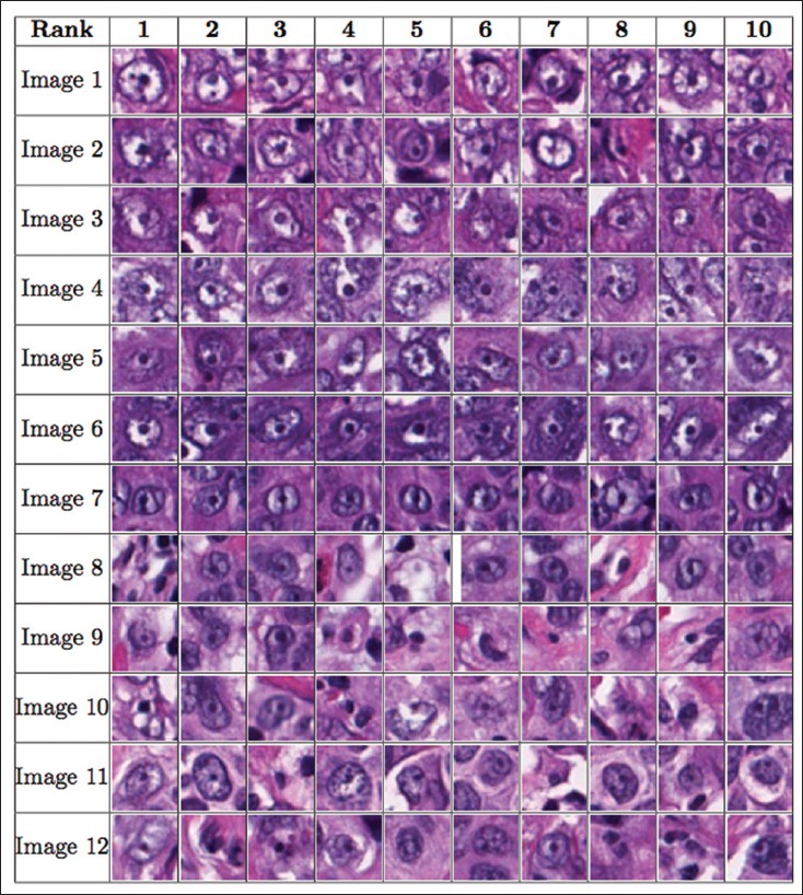
The figure shows the order of the ten most prominent nucleoli patterns to be presented to the pathologist for the breast cancer dataset

Renal Clear Cell Cancer Dataset

There were nine images in this dataset; we performed nine-fold cross-validation, training on eight images and testing on the remaining image. The image patch sizes used in this dataset were s × s = 12 × 12, 15 × 15, 18 × 18, 21 × 21, and 24 × 24. It was observed that our algorithm is ineffective for this dataset if only one image size of 24 × 24 pixels is used, perhaps due to varying sizes of prominent nucleoli patterns. Classifiers used in the cascade were HPG, EHPG, and XCA. LR was not used for this dataset for the same reasons as in the breast cancer dataset. Figure 7 shows that on average, the algorithm correctly detected about 86 prominent nucleoli patterns in the top 100 ranked detected objects. Figure 8 shows the top ten ranked image patches generated by our method accurately detects patterns of prominent nucleoli. The number of cascades for all Images 1–9 was 32. Our method missed 0.73% ± 0.44% of the total number of prominent nucleoli patterns.

Figure 7.

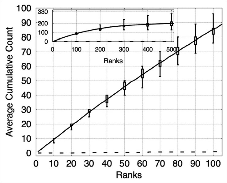
The plot shows the cumulative counts averaged over nine images versus ranks for prominent nucleoli patterns detected in the renal clear cell cancer dataset. The result for an algorithm that randomly ranks the pixels (dashed line) would fare much worse detecting only about 3.1% correct prominent nucleoli on average among its top 100 objects. The inset figure shows the average cumulative count curve for 500 ranked objects. The box plots indicate the first and third quarters of the data distribution. Horizontal bars show the highest and lowest cumulative counts

Figure 8.

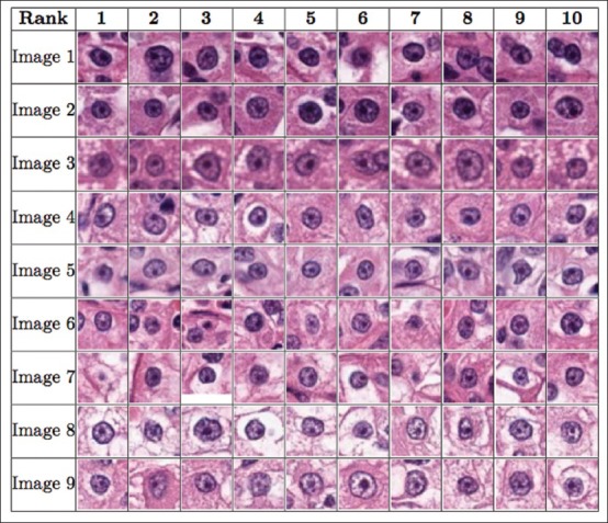
The figure shows the order of the ten most prominent nucleoli patterns to be presented to the pathologist for the renal clear cell cancer dataset

Renal Papillary Cell Cancer

There were nine images in this dataset; we performed nine-fold cross validation, training on eight images and testing on the remaining image. For testing Image 2, we used a positive retention rate of 1 while training the cascades and tested them on all the pixels. The image patch size used in this dataset was s × s = 24 × 24. Classifiers used in the cascade were HPG, EHPG, and XCA. LR was not used for this dataset for the same reasons as in the breast cancer dataset. In the EHPG classifier, 150 and 500 weak classifiers were used in the cascades. Figure 9 shows that on average the algorithm correctly detected about 76 prominent nucleoli patterns in the top 100 ranked detected objects. Figure 10 shows that the top ten ranked image patches generated by our method accurately detects patterns of prominent nucleoli. The number of cascades for Image 1 was 31, Images 2, 3, 4, and 5 was 32, Image 6 was 34, Image 7 was 33, Image 8 was 34, and Image 9 was 32. Our method missed 0.61 ± 0.53% of the total number of prominent nucleoli patterns.

Figure 9.

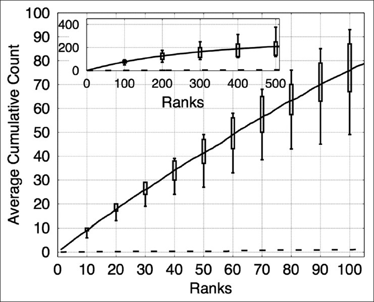
The plot shows the cumulative counts averaged over nine images versus ranks for prominent nucleoli patterns detected in the renal cell papillary cancer dataset. The result for an algorithm that randomly ranks the pixels (dashed line) would fare much worse detecting only about 1% correct prominent nucleoli on average among its top 100 objects. The inset figure shows the average cumulative count curve for 500 ranked objects. The box plots indicate the first and third quarters of the data distribution. Horizontal bars show the highest and lowest cumulative counts

Figure 10.

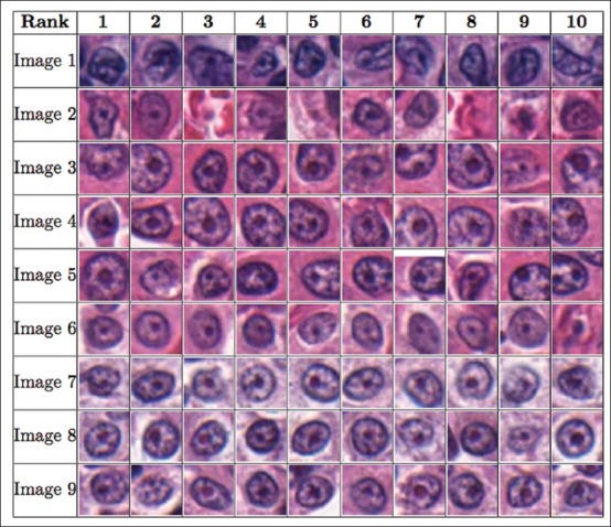
The figure shows the order of the 10 most prominent nucleoli patterns to be presented to the pathologist for the renal cell papillary cancer dataset

Effects of Using Different Number of Cascades and Different Combinations of Classifiers

To illustrate the purpose of different types of classifiers in the cascade, we studied the performance of our method under different cascade configurations. We started with only one cascade with XCA, HPG or EHPG classifiers and an image patch size of s × s = 24 × 24. The configurations with XCA only detected 45, with HPG only detected 35, and with EHPG only detected 51 prominent nucleoli patterns in the top 100 ranked detected objects, respectively. Using one classifier with one cascade for object detection follows the method proposed in Viola and Jones.[46] It is apparent that this method detects half the number of prominent nucleoli pattern compared to our cascade farm. We also combined five cascades at a time using either the EHPG or HPG classifier with image patch size of s × s = 12 × 12, 15 × 15, 18 × 18, 21 × 21, and 24 × 24. Under these multi-scale configurations, our method was able to detect 69 (EHPG only) and 65 (HPG only) prominent nucleoli patterns in the top 100 ranked detected objects. We also combined seven cascades using both EHPG and HPG classifiers with image patch size of s × s = 24 × 24. These seven cascades were in seven different color spaces. Using this configuration, our method detected 67 prominent nucleoli patterns in the top 100 ranked detected objects.

We also combined the above 18 (=1 + 5 × 2 + 7) cascades. This configuration led to the detection of 80 prominent nucleoli patterns in the top 100 ranked detected objects. These seven configurations for cascade combination were then compared with the final result of combining 32 cascades. Figure 2 compares these seven configurations with the best result of the 32-cascade combination. The final result of 32 cascades detected 86 prominent nucleoli patterns in the top 100 ranked detected objects.

Conclusion

We have shown in this paper that an accurate prominent nucleoli pattern detector can be built and potentially used routinely in clinics. To be used in diagnostics, however, for future work, a good user-friendly interface, parallelized implementation of our method, and efficient sample preparation and image acquisition methods need to be developed.

We have discovered two main factors that can further improve the accuracy of our methods– increase in number of cascades and use of multi-resolution image patches. More systematic and extensive studies of how these two factors affect system performance are in order for our future studies. However, these will increase training times significantly, and hence we omitted such detailed study in this paper.

With the current system configuration, training times over hundreds of cascades takes about a week but testing time is 2 min on an image of 1360 × 1024 pixels per cascade on the prostate dataset. To make our method viable for clinical application, since image patches are processed independently, the algorithm can be trivially parallelized. For example, using a small GPU machine cluster, each image patch can be processed independently and distributed to 10,000 GPU units (several thousand GPU units per machine and using tens of machines) to achieve three to four orders of magnitude speed up in computational time. Combining all image patterns using the RankBoost algorithm takes negligible time compared to that taken by the GPU cluster.

REFERENCES

- 1.Allsbrook WC, Jr, Mangold KA, Johnson MH, Lane RB, Lane CG, Amin MB, et al. Interobserver reproducibility of Gleason grading of prostatic carcinoma: Urologic pathologists. Hum Pathol. 2001;32:74–80. doi: 10.1053/hupa.2001.21134. [DOI] [PubMed] [Google Scholar]
- 2.Grossfeld GD, Chang JJ, Broering JM, Li YP, Lubeck DP, Flanders SC, et al. Under-staging and under grading in a contemporary series of patients undergoing radical prostatectomy: Results from the cancer of the prostate strategic urologic research endeavor database. J Urol. 2001;165:851–6. [PubMed] [Google Scholar]
- 3.Derenzini M, Montanaro L, Treré D. What the nucleolus says to a tumour pathologist. Histopathology. 2009;54:753–62. doi: 10.1111/j.1365-2559.2008.03168.x. [DOI] [PubMed] [Google Scholar]
- 4.Lorenzato M, Abboud P, Lechki C, Browarnyj F, O’Donohue MF, Ploton D, et al. Proliferation assessment in breast cancer: A double-staining technique for AgNOR quantification in MIB-1 positive cells especially adapted for image cytometry. Micron. 2000;31:151–9. doi: 10.1016/s0968-4328(99)00072-4. [DOI] [PubMed] [Google Scholar]
- 5.Montanaro L, Treré D, Derenzini M. Nucleolus, ribosomes, and cancer. Am J Pathol. 2008;173:301–10. doi: 10.2353/ajpath.2008.070752. [DOI] [PMC free article] [PubMed] [Google Scholar]
- 6.Rashid F, Ul Haque A. Frequencies of different nuclear morphological features in prostate adenocarcinoma. Ann Diagn Pathol. 2011;15:414–21. doi: 10.1016/j.anndiagpath.2011.06.002. [DOI] [PubMed] [Google Scholar]
- 7.Derenzini M, Trerè D, Pession A, Montanaro L, Sirri V, Ochs RL. Nucleolar function and size in cancer cells. Am J Pathol. 1998;152:1291–7. [PMC free article] [PubMed] [Google Scholar]
- 8.Derenzini M, Treré D, Pession A, Govoni M, Sirri V, Chieco P. Nucleolar size indicates the rapidity of cell proliferation in cancer tissues. J Pathol. 2000;191:181–6. doi: 10.1002/(SICI)1096-9896(200006)191:2<181::AID-PATH607>3.0.CO;2-V. [DOI] [PubMed] [Google Scholar]
- 9.Diaconescu S, Diaconescu D, Toma S. Nucleolar morphometry in prostate cancer. Bull Transilvania Univ Brasov. 2010;3:23–6. [Google Scholar]
- 10.Epstein JI, Cubilla AL, Humphrey PA. 1st ed. Annapolis Junction, Maryland: American Registry of Pathology; 2011. Tumors of the prostate gland, seminal vesicles, penis, and scrotum AFIP atlas of tumor pathology: Series 4. [Google Scholar]
- 11.Epstein JI. Diagnostic criteria of limited adenocarcinoma of the prostate on needle biopsy. Hum Pathol. 1995;26:223–9. doi: 10.1016/0046-8177(95)90041-1. [DOI] [PubMed] [Google Scholar]
- 12.Iczkowski KA, Bostwick DG. Criteria for biopsy diagnosis of minimal volume prostatic adenocarcinoma: Analytic comparison with nondiagnostic but suspicious atypical small acinar proliferation. Arch Pathol Lab Med. 2000;124:98–107. doi: 10.5858/2000-124-0098-CFBDOM. [DOI] [PubMed] [Google Scholar]
- 13.Varma M, Lee MW, Tamboli P, Zarbo RJ, Jimenez RE, Salles PG, et al. Morphologic criteria for the diagnosis of prostatic adenocarcinoma in needle biopsy specimens. A study of 250 consecutive cases in a routine surgical pathology practice. Arch Pathol Lab Med. 2002;126:554–61. doi: 10.5858/2002-126-0554-MCFTDO. [DOI] [PubMed] [Google Scholar]
- 14.Nickerson JA. Nuclear dreams: The malignant alteration of nuclear architecture. J Cell Biochem. 1998;70:172–80. [PubMed] [Google Scholar]
- 15.Kelemen PR, Buschmann RJ, Weisz-Carrington P. Nucleolar prominence as a diagnostic variable in prostatic carcinoma. Cancer. 1990;65:1017–20. doi: 10.1002/1097-0142(19900215)65:4<1017::aid-cncr2820650429>3.0.co;2-f. [DOI] [PubMed] [Google Scholar]
- 16.Helpap B. Observations on the number, size and localization of nucleoli in hyperplastic and neoplastic prostatic disease. Histopathology. 1988;13:203–11. doi: 10.1111/j.1365-2559.1988.tb02025.x. [DOI] [PubMed] [Google Scholar]
- 17.Demir C, Yener B. Automated Cancer Diagnosis Based on Histopathological Images: A Systematic Survey. Rensselaer Polytechnic Institute, Tech. Rep. 2005 [Google Scholar]
- 18.Irshad H, Veillard A, Roux L, Racoceanu D. Methods for nuclei detection, segmentation, and classification in digital histopathology: A review-current status and future potential. IEEE Rev Biomed Eng. 2014;7:97–114. doi: 10.1109/RBME.2013.2295804. [DOI] [PubMed] [Google Scholar]
- 19.Fuchs TJ, Buhmann JM. Computational pathology: Challenges and promises for tissue analysis. Comput Med Imaging Graph. 2011;35:515–30. doi: 10.1016/j.compmedimag.2011.02.006. [DOI] [PubMed] [Google Scholar]
- 20.Vink JP, Van Leeuwen MB, Van Deurzen CH, De Haan G. Efficient nucleus detector in histopathology images. J Microsc. 2013;249:124–35. doi: 10.1111/jmi.12001. [DOI] [PubMed] [Google Scholar]
- 21.Khurd P, Grady L, Kamen A, Gibbs-Strauss S, Genega EM, Frangioni JV. Chicago, Illinois, USA: Proceedings of 8th IEEE International Symposium on Biomedical Imaging: From Nano to Macro; 2011 Mar 30-Apr 2. IEEE; 2011. Network cycle features: Application to computer-aided gleason grading of prostate cancer histopathological images. [Google Scholar]
- 22.Doyle S, Feldman M, Tomaszewski J, Madabhushi A. A boosted Bayesian multiresolution classifier for prostate cancer detection from digitized needle biopsies. IEEE Trans Biomed Eng. 2012;59:1205–18. doi: 10.1109/TBME.2010.2053540. [DOI] [PubMed] [Google Scholar]
- 23.Rajpoot N, Arif M, Bhalerao AH. Proceedings of the British Machine Vision Conference; 2007 Sep 10-13. Warwick, UK: [Last cited on 2014 Apr 05]. Unsupervised Learning of Shape Manifolds. Available from: http://www.eprints.dcs.warwick.ac.uk/476/ [Google Scholar]
- 24.Arif M, Rajpoot N. Islamabad, Pakistan: Proceedings of International Conference on Machine Vision (ICMV); 2007 Dec 28-29. IEEE; Classification of potential nuclei in prostate histology images using shape manifold learning. [Google Scholar]
- 25.Tabesh A, Teverovskiy M, Pang HY, Kumar VP, Verbel D, Kotsianti A, et al. Multifeature prostate cancer diagnosis and Gleason grading of histological images. IEEE Trans Med Imaging. 2007;26:1366–78. doi: 10.1109/TMI.2007.898536. [DOI] [PubMed] [Google Scholar]
- 26.Diamond J, Anderson NH, Bartels PH, Montironi R, Hamilton PW. The use of morphological characteristics and texture analysis in the identification of tissue composition in prostatic neoplasia. Hum Pathol. 2004;35:1121–31. doi: 10.1016/j.humpath.2004.05.010. [DOI] [PubMed] [Google Scholar]
- 27.Naik S, Doyle S, Feldman M, Tomaszewski J, Madabhushi A. Gland Segmentation and Computerized Gleason Grading of Prostate Histology by Integrating Low-, High-Level and Domain Specific Information. MIAAB Workshop. 2007 [Google Scholar]
- 28.Nguyen K, Jain AK, Sabata B. Prostate cancer detection: Fusion of cytological and textural features. J Pathol Inform. 2011;2:S3. doi: 10.4103/2153-3539.92030. [DOI] [PMC free article] [PubMed] [Google Scholar]
- 29.Nguyen K, Jain AK, Allen RL. Istanbul, Turkey: Proceedings of 20th International Conference on Pattern Recognition (ICPR); 2010 Aug 23-26 IEEE; Automated gland segmentation and classification for Gleason grading of prostate tissue images. [Google Scholar]
- 30.Doyle S, Rodriguez C, Madabhushi A, Tomaszeweski J, Feldman M. New York, USA: Proceedings of 28th Annual International Conference of the IEEE Engineering in Medicine and Biology Society; 2006 Aug 30-Sep 3; IEEE; 2006. Detecting prostatic adenocarcinoma from digitized histology using a multi-scale hierarchical classification approach. [DOI] [PubMed] [Google Scholar]
- 31.Khurd P, Bahlmann C, Maday P, Kamen A, Gibbs-Strauss S, Genega EM, et al. Rotterdam, the Netherlands: Proceedings of IEEE International Symposium on Biomedical Imaging: From Nano to MacroMacro; 2010 Apr 14-17 IEEE; 2010. Computer-aided Gleason grading of prostate cancer histopathological images using texton forests. [DOI] [PMC free article] [PubMed] [Google Scholar]
- 32.Tahir MA, Bouridane A, Kurugollu F. An FPGA based coprocessor for GLCM and Haralick texture features and their application in prostate cancer classification. Analog Integr Circuits Signal Process. 2005;43:205–15. [Google Scholar]
- 33.Haralick RM, Shanmugam K, Dinstein IH. Textural features for image classification. IEEE Trans Syst Man Cybern. 1973;6:610–21. [Google Scholar]
- 34.Smith Y, Zajicek G, Werman M, Pizov G, Sherman Y. Similarity measurement method for the classification of architecturally differentiated images. Comput Biomed Res. 1999;32:1–12. doi: 10.1006/cbmr.1998.1500. [DOI] [PubMed] [Google Scholar]
- 35.Arif M, Rajpoot NM. Aberystwyth, UK: Proceedings of Medical Image Understanding and Analysis (MIUA); 2007. Jul 17-18, Detection of nuclei by unsupervised manifold learning. [Google Scholar]
- 36.Huang CH, Veillard A, Roux L, Loménie N, Racoceanu D. Time-efficient sparse analysis of histopathological whole slide images. Comput Med Imaging Graph. 2011;35:579–91. doi: 10.1016/j.compmedimag.2010.11.009. [DOI] [PubMed] [Google Scholar]
- 37.Huang PW, Lee CH. Automatic classification for pathological prostate images based on fractal analysis. IEEE Trans Med Imaging. 2009;28:1037–50. doi: 10.1109/TMI.2009.2012704. [DOI] [PubMed] [Google Scholar]
- 38.Tai SK, Li CY, Wu YC, Jan YJ, Lin SC. Seoul, South Korea: Proceedings of 6th International Conference on Digital Content Multimedia Technology and its Applications (IDC); 2006 Aug 16-18; IEEE; 2010. Classification of prostatic biopsy. [Google Scholar]
- 39.Hafiane A, Bunyak F, Palaniappan K. New York, USA: Proceedings of Microscopic Image Analysis with Applications in Biology; 2008. Sep 6, [Last cited on 2014 Jan 05]. Level set-based histology image segmentation with region-based comparison. Available from: http://www.miaab.org/miaab-2008-papers/15-miaab-2008-paper-14.pdf . [Google Scholar]
- 40.Jafari-Khouzani K, Soltanian-Zadeh H. Multiwavelet grading of pathological images of prostate. IEEE Trans Biomed Eng. 2003;50:697–704. doi: 10.1109/TBME.2003.812194. [DOI] [PubMed] [Google Scholar]
- 41.Yoon HJ, Li CC, Christudass C, Veltri R, Epstein JI, Zhang Z. Atlanta, Georgia, USA: Proceedings of IEEE International Conference on Bioinformatics and Biomedicine (BIBM); 2011 Nov 12-15; IEEE; 2011. Cardinal multiridgelet-based prostate cancer histological image classification for Gleason grading. [Google Scholar]
- 42.Roula M, Diamond J, Bouridane A, Miller P, Amira A. Washington, DC, USA: Proceedings of 2002 IEEE International Symposium on Biomedical Imaging; 2002 Jul 7-10; IEEE; 2002. A multispectral computer vision system for automatic grading of prostatic neoplasia. [Google Scholar]
- 43.Dalle JR, Leow WK, Racoceanu D, Tutac AE, Putti TC. Vancouver, British Columbia, Canada: Proceedings of 30th Annual International Conference of the IEEE Engineering in Medicine and Biology Society; 2008 Aug 20-24; IEEE; 2008. Automatic breast cancer grading of histopathological images. [DOI] [PubMed] [Google Scholar]
- 44.Ciresan DC, Giusti A, Gambardella LM, Schmidhuber J. Nagoya, Japan. Berlin Heidelberg: Proceedings of Medical Image Computing and Computer-Assisted Intervention-MICCAI 2013; 2013 Sep 22-26; Springer; 2013. Mitosis detection in breast cancer histology images with deep neural networks. [DOI] [PubMed] [Google Scholar]
- 45.Freund Y, Iyer R, Schapire RE, Singer Y. An efficient boosting algorithm for combining preferences. J Mach Learn Res. 2003;4:933–69. [Google Scholar]
- 46.Viola PA, Jones MJ. Robust real-time face detection. Int J Comput Vis. 2004;57:137–54. [Google Scholar]
- 47.Image J. Process Menu. [Last cited on 2013 May 05]. Available from: http://www.imagej.nih.gov/ij/docs/menus/process.html#find-maxima .
- 48.Rasband WS, Image J. Bethesda, Maryland, USA: U. S. National Institutes of Health; 1997-2014. [Last cited on 2013 May 05]. Available from: http://www.imagej.nih.gov/ij/ [Google Scholar]
- 49.Huang CH, Lee HK. Tsukuba Science City, Japan: Proceedings of 21st International Conference on Pattern Recognition (ICPR); 2012 Nov 11-15; IEEE; 2012. Automated mitosis detection based on exclusive independent component analysis. [Google Scholar]
- 50.Dalal N, Triggs B. San Diego, California, USA: Proceedings of IEEE Computer Society Conference on Computer Vision and Pattern Recognition (CVPR) 2005; 2005 Jun 20-25; IEEE; 2005. Histograms of oriented gradients for human detection. [Google Scholar]
- 51.Freund Y, Schapire RE. A decision-theoretic generalization of on-line learning and an application to boosting. J Comput Syst Sci. 1997;55:119–39. [Google Scholar]