Accelerated Molecular Dynamics Simulations of Protein Folding

Abstract

Folding of four fast-folding proteins, including chignolin, Trp-cage, villin headpiece and WW domain, was simulated via accelerated molecular dynamics (aMD). In comparison with hundred-of-microsecond timescale conventional molecular dynamics (cMD) simulations performed on the Anton supercomputer, aMD captured complete folding of the four proteins in significantly shorter simulation time. The folded protein conformations were found within 0.2–2.1 Å of the native NMR or X-ray crystal structures. Free energy profiles calculated through improved reweighting of the aMD simulations using cumulant expansion to the 2^nd order are in good agreement with those obtained from cMD simulations. This allows us to identify distinct conformational states (e.g., unfolded and intermediate) other than the native structure and the protein folding energy barriers. Detailed analysis of protein secondary structures and local key residue interactions provided important insights into the protein folding pathways. Furthermore, the selections of force fields and aMD simulation parameters are discussed in detail. Our work shows usefulness and accuracy of aMD in studying protein folding, providing basic references in using aMD in future protein-folding studies.

Graphical abstract

Introduction

Molecular dynamics (MD) simulations of biomolecules have often suffered from two major challenges: sufficient conformational sampling and accurate physical force fields^1,2. Despite remarkable advances in modern computing power, conventional MD (cMD) simulations are still limited to significantly shorter timescales than those displayed by many biomolecular motions and functions. This leads to poor conformational sampling of biomolecules such as proteins, nucleic acids and lipid membrane. In addition, development of accurate force fields, including the CHARMM³, AMBER⁴, OPLS-AA⁵ and GROMOS⁶, is normally subject to extensive validation with experimental data and iterative improvements, especially for the increasingly long-timescale MD simulations of biomolecules.

Protein folding is one of the most fundamental and fascinating biological processes. However, it remains a long-standing problem to understand the detailed mechanisms of protein folding from primary sequence to the native three-dimensional structures. A number of small proteins with ~10−100 amino acid residues fold on the microsecond to sub-millisecond timescales, known as “fast-folding” proteins. They serve as excellent model systems to study protein folding. Using the specialized supercomputer Anton, the DE Shaw Research Group performed all-atom cMD simulations on the hundreds-of-microsecond to millisecond timescales that captured spontaneous folding of 12 of such fast-folding proteins⁷, including the chignolin, Trp-cage, villin headpiece, WW domain, protein B/G and λ-repressor. Folding of chignolin^8,9, villin¹⁰, ubiquitin¹¹ and WW domain¹² has also been reported elsewhere through long-timescale cMD simulations in explicit water.

To properly describe the native structure and folding mechanism of a particular protein, the accuracy of the physical force field used is of capital importance. A number of force fields have been employed for different protein folding studies. This list includes: a modified CHARMM22 force field for 12 proteins including chignolin, Trp-cage, villin headpiece and WW domain;^7,13 with OPLS-AA force field it is possible to fold WW domain in less than 50 μs of cMD simulation;¹⁴ GROMOS 54A7 force field is able to fold small β-peptides;¹⁵ AMBER ff03 was used for villin;¹³ ff96 was employed for WW domain;¹⁶ and ff14SBonlysc was used to fold a diverse set of 17 fast-folding proteins.¹⁷ The force field bias and its implications for protein folding simulations have been extensively investigated^2,18–20. Ideally, one force field would describe the dynamics of all kinds of protein folding accurately, but it is common in practice that one force field is more optimized to certain protein systems or has the tendency to favor a certain secondary structure over another.¹⁸ Transferability of force field is still desirable, especially in the field of protein folding. Using a total of four different force fields (both AMBER and CHARMM), Piana et al. studied the folding pathways and native structure of villin headpiece, showing a good agreement of all force fields with experiments in obtaining the native structure, but significant discrepancies were found when examining folding mechanisms and properties of the unfolded state.¹³ To overcome these limitations, several efforts have been made to improve existing force fields in order to properly account for folding pathways more generally. In this line, Best and coworkers introduced simple corrections to AMBER ff99SB and ff03 force-fields to obtain an unbiased potential energy function^18,21 while Shaw et al. modified backbone torsional potentials of CHARMM22 to make this force field more transferable.¹³ There is still no consensus on which is the best choice but significant progress has been made towards more robust and transferable force fields. Lindorff-Larsen and coworkers performed a systematic study of different force-fields including AMBER, CHARMM and OPLS for a diverse set of proteins and compared the results with experimental measurements, finding modified versions of CHARMM (CHARMM22*) and AMBER (ff99SBILDN*) that better reproduce experimental data.¹⁴ The improvement and development of new force fields continues to be one of the current challenges of protein folding.

Protein folding requires an extensive amount of conformational sampling and computational power to properly characterize the free-energy landscape. Several techniques have proven appropriate to speed up simulations of folding and unfolding events. For example, Simmerling and coworkers merged implicit solvent models with graphical-processing units (GPU) to accelerate protein folding in a set of 17 fast-folding proteins obtaining roughly 1μs/day.¹⁷ By losing the atomistic description but gaining speed, Zhou et al. used the coarse-grained united-residue force field to successfully connect microscopic motions with experimental observations in WW domain providing relevant details on the folding kinetics.²²

In addition to cMD, protein folding has been studied using efficient sampling techniques such as replica-exchange MD²³, Markov State Models (MSM)²⁴ and biasing MD simulations such as bias-exchange metadynamics²⁵ and transition path sampling²⁶. For example, a combination of MSM and replica-exchange MD was used by Levy and coworkers to describe the folding pathways of Trp-Cage.²⁷ Laio and coworkers characterized the free-energy landscape of the third-Ig binding domain of protein G by means of NMR-guided metadynamics²⁸. While these simulations provided significantly enhanced conformational sampling of the proteins for folding, they require pre-defined reaction coordinates that place restraints on the protein folding, and the replica exchange methods suffer from the need of a large number of replicas for even the small, fast-folding proteins.

Accelerated molecular dynamics (aMD) is an enhanced sampling technique that works often by adding a non-negative boost potential to decrease the energy barriers and thus accelerate transitions between different low-energy states^29,30. With this, aMD is able to sample distinct biomolecular conformations and rare barrier-crossing events that are not accessible to cMD simulations. Unlike the above-mentioned biasing simulation methods, aMD does not require any pre-defined reaction coordinate(s). Thus, aMD can be advantageous for exploring the biomolecular conformational space without a priori knowledge or restraints. aMD has been successfully applied to a number of biological systems^31–35 and hundreds-of-nanosecond aMD simulations have been shown to capture millisecond-timescale events in both globular and membrane proteins^36,37. Doshi and Hamelberg observed folding of chignolin, Trp-cage and villin norleucine double-mutant through RaMD-db (a modified version of dual-boost aMD) simulations and achieved a speed-up of ~180 times in the folding of Trp-cage.³⁸

Here, aMD is further applied to simulate four fast-folding proteins that contain different characteristic secondary structures: the chignolin (β-hairpin or turn), Trp-cage (two α-helices), C-terminal fragment of the wild-type villin headpiece (three α-helices) and WW domain (three-stranded β-sheet). Therefore, the main aim of this work is to assess the validity of dual-boost aMD to predict the native structure and to properly retrieve the free-energy profile of a variety of proteins. Using cumulant expansion to the 2^nd order that greatly improves the accuracy of aMD reweighting³⁹, we successfully recovered the original free energy profiles of chignolin, Trp-cage, and villin that are comparable to those obtained from long-timescale Anton cMD simulations. Furthermore, aMD acceleration parameters are extensively explored for folding of the villin headpiece. Both villin and WW domain are simulated using different AMBER force fields because certain force fields such as AMBER ff03 are known to bias protein folding towards formation of α-helices^14,19. Additionally, for the WW domain simulations, we used two different aMD acceleration parameter sets: the set employed to fold chignolin and Trp-Cage simulations, and the set selected from villin simulations. In this work, we do not attempt to discuss the accuracy of different force fields; therefore, in the simulations of each protein we chose force fields validated in previous published studies for each particular case.

Methods

Accelerated Molecular Dynamics

Accelerated molecular dynamics (aMD) enhances the conformational sampling of biomolecules, often by adding a non-negative boost potential to the system when the system potential is lower than a reference energy^29,30,40:

$$\begin{array}{ll}{V}^{\ast }(\mathit{r})=V(\mathit{r}),\hfill & V(\mathit{r})\ge E,\hfill \\ V^{\ast }(\mathit{r})=V(\mathit{r})+\mathrm{\Delta }V(\mathit{r}),\hfill & V(\mathit{r})<E,\hfill \end{array}$$ (1)

where V (r) is the original potential, E is the reference energy, and V*(r) is the modified potential. In the simplest form, the boost potential, ΔV(r) is given by:

$$\mathrm{\Delta }V(\mathit{r})=\frac{{(E-V(\mathit{r}))}^2}{\alpha +E-V(\mathit{r})},$$ (2)

where α is the acceleration factor. As the acceleration factor α decreases, the energy barriers are decreased more and biomolecular transitions between the low-energy states are increased.

Two versions of aMD that provide different acceleration levels of biomolecules are termed “dihedral-boost”²⁹ and “dual-boost”³⁰. In dihedral-boost aMD, boost potential is applied to all dihedrals in the system with input parameters (E_dihed, α_dihed). In dual-boost aMD, a total boost potential is applied to all atoms in the system in addition to the dihedral boost, i.e., (E_dihed, α_dihed; E_total, α_total):

$$\begin{array}{ll}{E}_{\text{dihed}}=V_{\text{dihed\_avg}}+a_1\times N_{\text{res}},\hfill & {\alpha }_{\text{dihed}}=a_2\times N_{\text{res}}/5;\hfill \\ E_{\text{total}}=V_{\text{total\_avg}}+b_1\times N_{\text{atoms}},\hfill & {\alpha }_{\text{total}}=b_2\times N_{\text{atoms}}\hfill \end{array}$$ (3)

where N_res is the number of protein residues, N_atoms is the total number of atoms, and V_{dihed_avg} and V_{total_avg} are the average dihedral and total potential energies calculated from short cMD simulations, respectively. The coefficients (a₁, a₂; b₁, b₂) that are used in the aMD simulations of chignolin, Trp-cage, villin and WW domain are listed in Table 1. Recently, Doshi and Hamelberg proposed to accelerate only rotatable torsions within the framework of the dual-boost approach,⁴¹ which was shown to enhance conformational sampling of protein folding.³⁸

Table 1.

Summary of the aMD simulations with best-chosen aMD parameters.

System	Nres	Natoms	Force Field	aMD	(a1, a2; b1, b2)
Chignolin	10	6,773	Amber ff99SB	300ns x3	(3.5, 3.5; 0.175, 0.175)
Trp-cage	20	34,370	Amber ff99SB	500ns x4	(3.5, 3.5; 0.175, 0.175)
Villin	35	33,915	Amber ff03	500ns x9	(4.0, 4.0; 0.3, 0.3)
WW domain	35	26,497	Amber ff96	500ns x10	(4.0, 4.0; 0.3, 0.3)

Energetic Reweighting

Details of different aMD reweighting methods are described in Ref. 39 and a brief summary is provided here. For aMD simulation of a biomolecular system, the probability distribution along a selected reaction coordinate A(r) is written as p^*(A), where r denotes the atomic positions {r₁,…,r_N}. Given the boost potential ΔV(r) of each frame, p^*(A) can be reweighted to recover the canonical ensemble distribution, p(A), as:

$$p(A_j)=p^{\ast }(A_j)\frac{{\langle e^{\beta \mathrm{\Delta }V(\mathit{r})}\rangle }_j}{{\displaystyle \sum _{j=1}^M{\langle e^{\beta \mathrm{\Delta }V(\mathit{r})}\rangle }_j}},j=1,\cdots ,M,$$ (4)

where M is the number of bins and ${\langle e^{\beta \mathrm{\Delta }V(\mathit{r})}\rangle }_j$ is the ensemble-averaged Boltzmann factor of ΔV(r) for simulation frames found in the j^th bin. The above equation provides an “exponential average” algorithm for aMD reweighting of aMD simulations. The reweighted potential of mean force (PMF) is calculated as $F(A_j)=-\frac{1}{\beta }\ln p(A_j)$.

As the Boltzmann factors are often dominated by high boost potential frames that are poorly sampled, the aMD reweighting based on exponential average generally leads to high energetic fluctuations^39,42. To reduce the energetic noise, the exponential term can be approximated as summation of the Maclaurin series of boost potential ΔV(r) and the reweighting factor is rewritten as:

$$\langle e^{\beta \mathrm{\Delta }V}\rangle ={\displaystyle \sum _{k=0}^{\infty }\frac{{\beta }^k}{k!}\langle \mathrm{\Delta }{V}^k\rangle }$$ (5)

where the subscript j has been suppressed. The Maclaurin series expansion up to the 5^th–10^th order has been used in practice to reweight aMD trajectories³⁶. The reweighted PMF profiles are typically less noisy than those obtained from exponential average reweighting, but lead to shifted energy minimum positions compared with the original profiles.

Furthermore, the ensemble-averaged reweighting factor can be approximated using a cumulant expansion^43,44:

$$\langle e^{\beta \mathrm{\Delta }V}\rangle =\exp \left\{{\displaystyle \sum _{k=1}^{\infty }\frac{{\beta }^k}{k!}{C}_k}\right\},$$ (6)

where the first three cumulants are given by:

$$\begin{array}{l}{C}_1=\langle \mathrm{\Delta }V\rangle ,\\ C_2=\langle \mathrm{\Delta }{V}^2\rangle -{\langle \mathrm{\Delta }V\rangle }^2={\sigma }_{\mathrm{\Delta }V}^2,\\ C_3=\langle \mathrm{\Delta }{V}^3\rangle -3\langle \mathrm{\Delta }{V}^2\rangle \langle \mathrm{\Delta }V\rangle +2{\langle \mathrm{\Delta }V\rangle }^2.\end{array}$$ (7)

As shown earlier, when the boost potential follows near-Gaussian distribution, cumulant expansion to the second order provides more accurate reweighting than the exponential average or the Maclaurin series expansion methods³⁹ and is thus used in this study.

System Preparation

The simulated systems were built using the Xleap module of the AMBER package. Chignolin with a sequence of ten residues (GYDPETGTWG) was constructed as described previously⁴⁵. For Trp-cage, the amino acid sequence was obtained from the PDB code 2JOF⁴⁶ and an extended polypeptide was built as the simulation starting structure. For the wild-type villin headpiece, the thirty-five amino acid sequence was extracted from the PDB code 1YRF.⁴⁷ Then, an extended polypeptide based on this sequence was used as starting point in our simulations. For the WW domain, the thirty-five amino acid sequence was obtained from Lindorff-Larsen et. al.⁷ as (GSKLPPGWEKRMSRDGRVYYFNHITGTTQFERPSG) and the extended structure of this sequence was also prepared as the starting structure of present simulations. After initial equilibrations (described in Simulation Protocols), the final chignolin system contained 2,211 waters, 11,355 waters for Trp-cage, 11,077 waters for villin and 8,644 waters for WW domain by solvating the equilibrated structures in a TIP3P⁴⁸ water box that extends 8 to 12 Å from the solute surface. The total number of atoms in the four systems are 6,773, 34,370, 33,915 and 26,497 for chignolin, Trp-cage, villin and WW domain, respectively (Table 1).

Simulation Protocols

Chignolin and Trp-cage were simulated using AMBER 12 package with the ff99SB force field on GPUs^4,49–51 using the SPFP precision model⁵². But for wild-type villin simulations, two AMBER force fields are tested, that is, ff03 and ff14SB. We chose ff03 as it has been extensively validated for folding of both wild-type and norleucine double mutant villin.^18,53 In a recent study, Lindorf-Karsten et al. showed that it is possible to simulate the folding of villin norleucine double mutant in less than 10μs using the ff03 force field.¹⁴ We also employed the recently proposed ff14SB, which is similar to ff99SB, but with new side chain and backbone dihedral parameters, and particularly designed to improve the agreement between experiments and simulations in explicit water (simulations with ff14SB force field have been carried out within the AMBER14 package). A similar force field, the ff14SBonlysc (ff99SB force field with only side chain dihedral parameters from ff14SB), was recently used to successfully simulate folding of villin and sixteen other proteins using implicit solvent exhibiting more transferability than ff03.¹⁷ For WW domain, three different AMBER force fields (ff96, ff99SB, and ff03) were employed. It is known that different AMBER force fields have different propensities for secondary structures; an old parameter set, ff96, is biased towards β-sheet structure^21,54,55 and ff03 overstabilizes helical structures.¹⁴ Thus, we tested the ff96, ff99SB, and ff03 force fields, using a native structure as the initial structure of cMD simulations, prepared from the PDB code 2F12⁵⁶. The 400 ns cMD simulations of three force fields showed that the native structures are very stable for all the cases in that C_α-atom RMSDs are small (<3 Å) (see Fig. S1.). Since this result does not conclude which force field is the best choice, we used all three force fields for WW domain folding simulations starting from the extended polypeptide.

In the AMBER simulations of the four systems, bonds containing hydrogen atoms were restrained with the SHAKE algorithm⁵⁷ and thus a 2 fs timestep was used. Weak coupling to an external temperature and pressure bath was used to control both temperature and pressure⁵⁸. The electrostatic interactions were calculated using the PME (particle mesh Ewald summation)⁵⁹ with a cutoff of 8.0 Å for chignolin and Trp-cage and 10.0 Å for villin and WW domain for long-range interactions.

To run aMD simulations, we first equilibrated the systems and used cMD simulations to calculate the aMD acceleration parameter sets. For equilibration, we repeated the following minimization-heating-simulation procedures twice: first, for the initial fully-extended conformation of the protein, and second, for the collapsed or more compact conformation of protein obtained from the first equilibration. That is, when a protein was collapsed from the extended form in a water bath during the first equilibration, we extracted the protein and resolvated it in a smaller water box. In this way, we reduced the total system size and accordingly we were able to save computational cost. In the first equilibration procedure, the four systems were initially minimized using conjugate gradient or steepest descent minimization algorithms, first with the solute atoms fixed and then with all atoms free. After energy minimization, the systems were slowly heated to 300 K. Then molecular dynamics simulations were performed in the isothermal-isovolumetric (NVT) ensemble (300 K) for chignolin, Trp-cage, and villin or in the isothermal-isobaric (NPT) ensemble (300K and 1 bar) for WW domain. For NVT simulations, before production simulation runs, system equilibration was achieved by a 200 ps NVT and 400 ps NPT run to assure that the water box of simulated systems had reached the appropriate density. We ran the simulations until the protein reduced its volume in solution (lower radius of gyration), whose simulation time is longer than 20 ns, and then we extracted the protein structure and solvated it with the aforementioned number of water molecules described in System Preparation. The second equilibration procedure was the same as the first one with the only exception of the cMD simulation time. We ran longer cMD simulations (>~50 ns) for calculating aMD acceleration parameters according to Eqs. (1)–(3).

Restarting from the final structures of cMD simulations, three independent 300 ns dual-boost aMD simulations were performed for chignolin and four independent 500 ns dual-boost aMD simulations for Trp-cage. For the wild-type villin, two independent 200 ns simulations were carried out using the ff03 force field for a wide range of acceleration parameters in order to select the most appropriate set. Then, with the most suitable parameter set nine independent 500 ns simulations were performed using the ff03 force field, while three independent 1,500 ns simulations were obtained by means of the ff14SB force field. For WW domain, ten independent 500 ns simulations were carried out using the ff96 force field, while two independent 500 ns simulations for ff99SB and ff03 force fields were also performed. In aMD simulations of the chignolin, Trp-cage and villin, trajectory frames were saved every 0.2 ps for proper reweighting unless noted otherwise. In the aMD simulations of the WW domain, frames were saved every 1 ps for analysis. A summary of the major simulations is listed in Table 1.

Simulation Analysis

The root-mean square deviation (RMSD) between aMD simulation snapshots and the PDB native structure, and the radius of gyration (R_g) were computed using the ptraj tool⁴ or VMD⁶⁰. Excluding the flexible N- and C-terminal residues, RMSDs were calculated using the C_α atoms of residues Tyr2-Trp9 in chignolin, Leu2-Pro18 in Trp-cage, and Pro5-Phe30 in WW domain. Notably, the folding free energy profiles of Trp-cage for calculating the RMSD with and without the heavy atoms in the Trp6 residue are closely similar to each other as demonstrated on the 208,000 ns Anton cMD simulation (see Figs. S7a–b). Thus further analysis of the Trp-cage simulations is performed using the only the C_α atoms of residues Leu2-Pro18 to calculate the protein RMSD. All residues were considered in villin. Protein secondary structures are analyzed using do_dssp in the GROMACS package⁶¹. A toolkit of Python scripts “PyReweighting” was used to reweight the aMD simulations³⁹ to calculate the potential of mean force (PMF) profiles. Cumulant expansion to the 2^nd order, which has been shown to greatly improve the reweighting of the aMD simulations³⁹, was applied in this study. As demonstrated on Trp-cage, compared with reweighting using cumulant expansion to the 2^nd order (Fig. 2b), the exponential average leads to highly noisy PMF (Fig. S7c). While the Maclaurin series expansion greatly suppresses the energetic noise, the resulting PMF deviates in the energy minimum positions and energy barrier values (Fig. S7d). A bin size of 0.5 Å is used for RMSD and R_g for the reweighting calculations. When the number of simulation frames within a bin is lower than a certain limit (i.e., cutoff), the bin is not sufficiently sampled and thus excluded for reweighing. The cutoff can be determined by iteratively increasing it until the minimum position of the PMF profile does not change. The final cutoff was set as 100, 800 and 2,400 for reweighting of aMD simulations on chignolin, Trp-cage and villin, respectively.

Fig. 2.

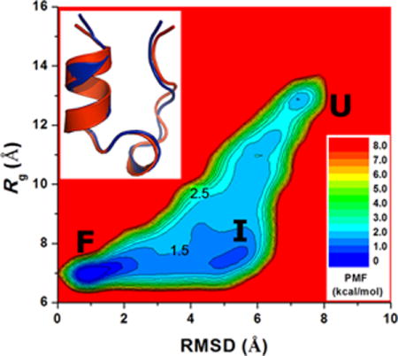
Folding of Trp-cage simulated via aMD: (a) comparison of simulation-folded Trp-cage (blue) with the PDB (2JOF) native structure (red) that exhibits 0.8 Å RMSD at t=120 ns in Sim1 (Fig. S4), (b) two-dimensional (RMSD, R_g) free energy profiles calculated by reweighting the four 500 ns aMD simulations combined, structural representations of the (c) folded (“F”), (d) unfolded (“U”) and (e) intermediate (“I”) states (blue) aligned to the native structure (red), and (f) time evolution of the protein secondary structure during the 500 ns aMD simulation containing the folded structure shown in (a), in which the α-helix (blue) starts to form at ~ 65 ns.

Results

Folding was observed in long-timescale aMD simulations of four fast-folding proteins: chignolin, Trp-cage, wild-type villin headpiece and WW domain. RMSDs of the proteins relative to the experimentally determined native structures were found to reach values within 0.2–2.1 Å. Moreover, we performed local structure comparison using the characteristic structure motifs, the secondary structure (SS) such as α helix and β sheets. When the proteins are in native states (low RMSD), we found that they have similar secondary structures to the native structures. In addition to the native structures, we also identified distinct protein conformations (e.g., intermediate and unfolded) from the reweighted free energy profiles for chignolin, Trp-cage and villin headpiece.

Chignolin

During each of the three independent 300 ns aMD simulations of chignolin, we observed folding of the protein multiple times with the RMSD decreasing to <2 Å relative to the native NMR structure (Fig. S2a). Fig. 1a shows the comparison between simulation-folded chignolin with the PDB native structure that exhibits 0.2 Å RMSD. Chignolin also becomes more compact during folding with the R_g of the protein decreasing to ~4.2 Å (Fig. S2b). Using the RMSD and R_g, two-dimensional PMF profiles were calculated by reweighting the three 300 ns aMD simulations combined. From the resulting free energy profiles (Fig. 1b), two distinct low-energy conformational states can be identified as the folded (“F”) and unfolded (“U”). The folded state corresponds to the global energy minimum at (0.5 Å, 4.0 Å). The unfolded state is 3.26 kcal/mol higher in a local energy well centered at (4.0 Å, 5.5 Å). The energy barrier for chignolin folding between the two conformational states is ~3.5 kcal/mol.

Fig. 1.

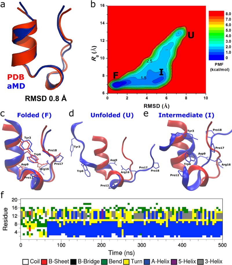
Folding of chignolin simulated via accelerated molecular dynamics (aMD): (a) comparison of simulation-folded chignolin (blue) with the PDB (1UAO) native structure (red) that exhibits 0.2 Å RMSD at t=50 ns in Sim1 (Fig. S2), (b) two-dimensional (RMSD, R_g) free energy profiles calculated by reweighting the three 300 ns aMD simulations combined, structural representations of the (c) folded (“F”) and (d) unfolded (“U”) states (blue) aligned to the native structure (red), and (e) time evolution of the protein secondary structure during the 300 ns aMD simulation containing the folded structure shown in (a), in which turn (yellow) is formed in the C-terminal (Trp9 and Thr8) and central (Gly7-Pro4) regions.

In the aMD simulation-derived folded state of chignolin, while Trp9 appears flexible near the C-terminus, the protein residue side chains exhibit closely similar conformations as in the NMR native structure (Fig. 1c). Notably, residues Tyr2 and Pro4 form hydrophobic interactions between their side chains. Hydrophilic residues Asp3, Glu5, Thr6 and Thr8 expose the side chains to the solvent. In the unfolded state, although the side chains of Tyr2 and Pro4 interact with each other, the protein does not form proper secondary structure in the central region and chignolin remains disordered (Fig. 1d).

Fig. 1e plots the time evolution of the protein secondary structure of chignolin during one of the three 300 ns aMD simulations (see Fig. S3 for all three independent simulations). It is important to note that the turn conformation is formed in the C-terminal (Trp9 and Thr8) and central (Gly7-Pro4) regions during folding of chignolin, but not in the N-terminal region. Moreover, the formation of turn in residues Trp9-Thr8 appears to precede that in Gly7-Pro4 (Fig. 1e), suggesting that turn is propagated from the C-terminus to the central region for folding of chignolin. This is consistent with previous finding from microsecond-timescale cMD simulations that the β-hairpin in chignolin forms by rolling up from the N-terminal strand⁹.

Trp-cage

For Trp-cage, the protein RMSD relative to the experimental native structure (the first NMR structure from PDB: 1L2Y) decreases to <2 Å multiple times during each of the four independent 500 ns aMD simulations (Fig. S4a). In Fig. 2a, the simulation-folded Trp-cage is compared with the PDB native structure, which exhibits 0.8 Å RMSD between the two structures. With the RMSD and R_g, a two-dimensional PMF profile was obtained by reweighting the four 500 ns aMD simulations combined (Fig. 2b). The global free energy minimum is located at (0.5 Å, 7.0 Å), corresponding to the folded (“F”) state. The unfolded (“U”) state exhibits a local energy well of 1.73 kcal/mol centered at (7.0 Å, 13.0 Å). In addition, an intermediate (“I”) state is identified centered at (5.0 Å, 7.5 Å); its free energy is 1.23 kcal/mol higher than the folded state. The energy barriers between the intermediate and the unfolded and folded states are estimated to be ~2.5 kcal/mol and ~1.5 kcal/mol, respectively.

In the folded state as shown in Fig. 2c, residues Trp6 and Tyr3 from the N-terminal α-helix, Pro12 from the central helix and Pro18 from the C-terminal region constitute the hydrophobic core of Trp-cage. Hydrophilic residues Asp9 and Arg16 expose their side chains to the solvent as in the experimental native structure. In the unfolded state, Trp-cage exhibits overall disordered secondary structures although residues Asp9 and Arg16 form transient salt bridge interactions (Fig. 2d). In the intermediate state, while Trp-cage has become compact with ~7.5 Å R_g, which is slightly greater than the native structure (7.0 Å), the protein RMSD relative to the native NMR structure is 4.5−5.5 Å (Fig. 2e). This state has also been identified in a previous study using bias exchange metadynamics simulations²⁵. Notably, Trp6 interacts strongly with Pro12 from the central helix in the intermediate state.

The time evolution of the protein secondary structure during the 500 ns aMD simulation containing the native structure shown in Fig. 2a is plotted in Fig. 2f (see Fig. S5 for data of all four independent aMD simulations). Started from the extended conformation, Trp-cage remains disordered during the beginning of the aMD simulation. The α-helix conformation is first formed at ~65 ns in the protein N-terminal region (residues Leu2-Asp9) and then in the central region (Pro12-Gly15). While the N-terminal helix is maintained until the end of the 500 ns aMD simulation, the central region transitions frequently between the helical and disordered conformations. This suggests that the N-terminal helix is significantly more stable than the central helix in Trp-cage. Similar trend was observed in the other three independent aMD simulations (Fig. S5).

Villin

Compared with chignolin and Trp-cage, villin poses additional challenges for modeling: the polypeptide chain is considerably longer (thirty-five residues), three α-helices are formed during the folding process, and folding time is over 10 μs. First, we focus on the ability of aMD to efficiently explore villin’s conformational space and to rapidly identify the folded native state. We initially carried out two independent simulations with the same parameters used for chignolin and Trp-cage (that is, a₁=3.5, a₂=3.5; b₁=0.175, b₂=0.175), but folding was not observed during 500 ns of aMD simulation. The lowest protein RMSD with respect to the experimental structure was found to be >4 Å. To overcome this situation, we decided to selectively tune acceleration parameters to further enhance conformational sampling and be able to observe folding events in a more accessible simulation time. To this end, we systematically screened a large set of aMD parameters that encompass different levels of acceleration. A total of four parameters were considered (see Eq. 3), a₁ that controls the value of E_dihedral, a₂ that regulates acceleration parameter α_dihedral, b₁ that controls E_total, and b₂ that assigns the value of α_total. The pairs a₁ and a₂, and b₁ and b₂ are usually treated with the same value (e.g. 3.5 for a₁ and a₂). Therefore, only two parameters are essentially required to perform aMD simulations. Here, we considered several combinations of parameters including some that use different values for b₁ and b₂. As Table 2 shows, we tested a broad range of parameters that span from 3.0 to 5.0 for dihedral boost parameters (a₁ and a₂) and from 0.15 to 0.5 for total boost (b₁ and b₂). Our criterion was to identify a set of aMD parameters that allow us to observe a single folding event in less than 200 ns of aMD. To this end, we ran two independent 200 ns simulations for each parameter set and we plotted the RMSD with respect to the experimental structure along the trajectory. All results obtained are summarized in Table 2, where best RMSD and average total and dihedral boost potentials (in kcal/mol) are given for each set of parameters. Interestingly, using 4.0 for a₁ and a₂ and 0.3 for b₁ and b₂ we were able to fold wild-type villin in less than 200 ns. The lowest protein RMSD observed in these 200 ns simulations was 0.91 Å. Then we set up nine-independent 500 ns simulations observing two folding events in total, 0.45 Å being the lowest value detected (see Fig. 3a). In both cases, the protein remains in the folded state for roughly 100 ns (see Fig. S8a). In the remaining seven trajectories the native structure is not identified within 500 ns of aMD and the system remains either unfolded or trapped in a partially folded intermediate state (see Fig. 3). Besides the (4.0,4.0;0.3,0.3) parameter combination, we were also able to observe folding events below 200 ns using other combinations of parameters as 4.0 (a₁/a₂) and 0.25 (b₁/b₂) obtaining an RMSD of 0.68 Å and 3.5 (a₁/a₂) and 0.3 (b₁/b₂) with an RMSD of 0.52 Å. These results indicate that our goal of folding wild-type villin below 200 ns of aMD was quite ambitious but at the same time we prove that it is clearly feasible. In addition, Table 2 shows a tendency to obtain lower RMSD values when the boost potential increases. For example, by using the (3.5,3.5;0.15,0.15) parameter set the lowest RMSD after 200 ns is 3.73 Å while RMSD is significantly lowered to 0.52 Å when b₁ and b₂ parameters are increased to 0.3 (see Table 2). This may be interpreted as a sign of a significant enhancement in conformational sampling although longer simulations will be required to properly assess this trend. In general, our results are in line with Doshi and Hamelberg, who performed RaMD-db simulations on the norleucine double mutant at 360K.³⁸ They observed folding events in about 200–300 ns of RaMD-db. Results are not strictly comparable since we focused on the wild type protein, which requires a longer time to fold into the native state. In addition, we performed our simulations at 300K with a different number of water molecules and employing a different force field. Interestingly, by utilizing more aggressive acceleration parameters we are still able to identify the native state. However, the use of large boost potentials may turn the reweighting of the free-energy profile into a daunting task.

Table 2.

Summary of the a₁, a₂, b₁, b₂ parameters screened for villin simulations. Two independent 200ns simulations of each parameter set were run. The lowest RMSD is shown in the table. Folded simulations are highlighted in bold. Average values of total boost potential and dihedral boost potential are represented (kcal/mol).

System	(a1, a2; b1, b2)	RMSD	Total Boost Potential	Dihedral Boost Pot
Villin	3.5, 3.5; 0.15,0.15	3.729	33.71	6.72
	3.5, 3.5; 0.175,0.175	4.047	52.37	7.09
	3.5, 3.5; 0.20,0.20	3.212	76.61	6.29
	3.5, 3.5; 0.25,0.25	1.624	143.68	6.04
	3.5, 3.5; 0.30,0.30	0.524	239.05	5.99
	4.0, 4.0; 0.15, 0.15	3.548	33.65	10.18
	4.0, 4.0; 0.175, 0.175	3.272	52.21	8.78
	4.0, 4.0; 0.20, 0.20	3.456	76.29	8.52
	4.0, 4.0; 0.25, 0.25	0.684	143.01	8.36
	4.0, 4.0; 0.30, 0.30	0.914	238.06	8.00
	4.5, 4.5; 0.15, 0.15	4.741	33.34	12.94
	4.5, 4.5; 0.175, 0.175	4.564	51.85	11.68
	4.5, 4.5; 0.20, 0.20	2.874	76.08	12.45
	4.5, 4.5; 0.25, 0.25	3.934	142.85	11.41
	4.5, 4.5; 0.30, 0.30	3.688	237.26	9.88
	3.0, 3.0; 0.15,0.15	4.365	33.78	5.42
	3.0, 3.0; 0.175,0.175	6.305	59.78	4.78
	4.0, 4.0; 0.30, 0.175	3.578	154.75	6.75
	4.0, 4.0; 0.30, 0.20	3.635	172.79	7.57
	4.0, 4.0; 0.30, 0.25	2.176	207.05	7.25
	5.0, 5.0; 0.50, 0.50	4.811	931.67	10.45

Fig. 3.

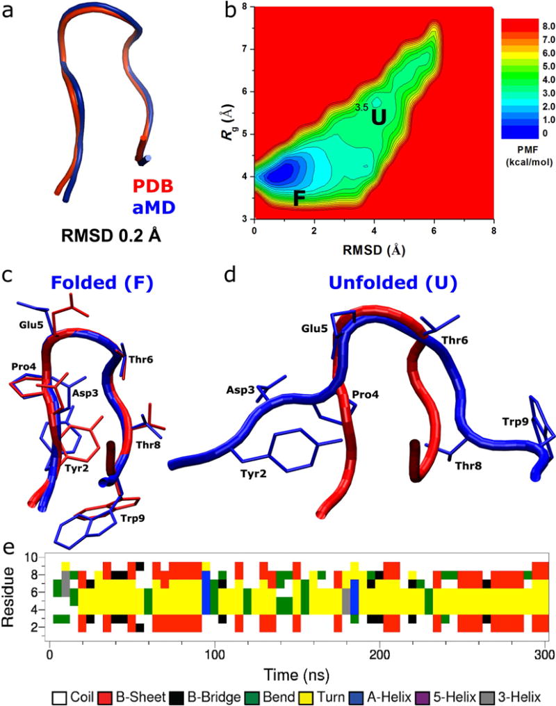
Folding of wild-type villin simulated via aMD: (a) comparison of simulation-folded villin using ff03 force field (blue) with the PDB (1YRF) native structure (red) that exhibits 0.45 Å RMSD at t=250 ns, (b) two-dimensional (RMSD, R_g) free energy profiles calculated by reweighting the nine 500 ns aMD simulations combined using ff03 force field, (c) folded (“F”), (d) intermediate (“I”), and (e) unfolded (“U”) states (blue) aligned to the native structure (red), (f) time evolution of the protein secondary structure during the 500 ns aMD simulation containing the folded structure shown in (a), (g) comparison of simulation-folded villin using ff14SB force field (blue) with the PDB (1YRF) native structure (red) that exhibits 0.40 Å RMSD at t = 500 ns, (h) two-dimensional (RMSD, R_g) free energy profiles calculated by reweighting the three 1500 ns aMD simulations combined using ff14SB force field, (i) folded (“F”), and (j) intermediate (“I”) states (blue) aligned to the native structure (red).

Reweighting villin simulations may present more complications considering the size of the system, the observed folding time, and the higher boost potential applied with respect to chignolin and Trp-cage simulations. In Fig. 3b, a two dimensional PMF profile (RMSD and R_g) is obtained by reweighting nine 500 ns villin simulations (all data comes from five simulations which were saved every 0.2 ps and four simulations saved every 2 ps). Interestingly, three minima corresponding to the folded, intermediate and unfolded states can be clearly identified. The global free-energy minimum “F” is found at (2.0 Å, 9.8 Å). An intermediate state centered at (6.5 Å, 8.8 Å) is found to be approximately 1 kcal/mol higher in energy than the native state while the unfolded state is located in the vicinity of (8.4 Å, 13.2 Å) in an energy well of 2 kcal/mol. The energy barriers between the intermediate and folded states and between the folded and unfolded states are estimated to be ~ 3 kcal/mol and ~ 4 kcal/mol respectively. In the folded state as shown in Fig 3c, residues Phe6 and Phe10 from N-terminal helix-1 and Phe17 from central helix-2 constitute the hydrophobic core of the villin headpiece. The orientations of these three residues found in the folded aMD structure (blue) are clearly in agreement with the experimental crystal structure (red). In the intermediate state (see Fig 3d) the three helices are completely folded and the protein structure remains compact but helix-1 is pointing in the opposite direction with respect to the folded state. This breaks the hydrophobic core and only Phe17 keeps a similar orientation as in the native state while Phe6 and Phe10 are exposed towards the solvent. In the unfolded state shown in Fig 3e the three helices are essentially unstructured. The PMF built from Anton simulations with CHARMM22* force field clearly sample a broader range of R_g and RMSD values (see Fig. S6c). The global free-energy minimum and the intermediate state are located at similar positions as our reweighted aMD simulations. Some differences may arise considering that Anton simulations were run for norleucine double mutant, which folds five times faster than the wild-type. In addition, we used a different force-field and different simulation temperature. It is well established that ff03 force stabilizes α-helices making intermediate and folded states significantly stable in comparison to other protein conformations. Clearly, our ff03 aMD simulations sample a smaller region of the conformational space compared to Anton simulations.

To understand the discrepancies in conformational sampling between ff03 aMD and Anton simulations, we carried out a number of villin aMD simulations with an additional force field. Recently, Simmerling and coworkers proved the validity of ff14SBonlysc force-field to fold villin and a diverse set of proteins in implicit solvent.¹⁷ By using the (4.0,4.0;0.3,0.3) parameter set we ran a total of three 1,500 ns independent aMD simulations with ff14SB (see Table 3). In all cases we observed the first folding event around 400 – 600 ns (see Fig. S8b) being 0.4 Å the best RMSD (see Fig. 3g). To analyze the differences between ff03 and ff14SB force fields, we computed the two-dimensional PMF combining the three independent simulations for a total of 4.5 μs (see Fig. 3h). Interestingly, the shape of the PMF significantly expands with respect to the one obtained with the ff03 force field indicating a noticeable increase in conformational sampling. In addition, more than one folding and unfolding event is observed in the course of the simulation (see Fig. S8b). The three critical points are located at similar positions, that is, the folded state is centered at (1.5 Å, 9.0 Å), the intermediate is found at (6.5 Å, 9.0 Å), while the unfolded state is slightly displaced (11.0 Å, 16.5 Å) with respect to ff03 simulations. For the ff14SB case, the intermediate state is found to be approximately 1.5 kcal/mol higher than the folded state while the energy barrier between the folded and intermediate states is about 2 kcal/mol. The aMD structures of the folded (see Fig. 3i) and intermediate (see Fig. 3j) states are similar to those obtained with the ff03 force field. The shape of the PMF clearly mirrors the one obtained from the Anton simulations for norleucine double mutant (see Fig. S6c).

Table 3.

Different force fields, parameters tested on Villin and WW domain.

System	force field, (a1, a2, b1, b2)
Villin	ff03, (4.0, 4.0; 0.3, 0.3)*
	ff14SB, (4.0, 4.0; 0.3, 0.3)
WW domain	ff03, (3.5, 3.5; 0.175, 0.175)
	ff99SB, (4.0, 4.0; 0.3, 0.3)
	ff96, (4.0, 4.0; 0.3, 0.3)

^*representative set; for other sets, see Table 2

We also analyzed the patterns of secondary structure along one of the aMD trajectories, which contains the native structure shown in Fig. 3a. From Fig. 3f we can see how helix 3 is the most stable and the helix that forms first in the very beginning of the aMD simulations. Then helices 1 and 2 alter their formation until the final three α-helix protein is folded into its native state. The folding mechanism of villin headpiece was deeply studied by Harada and coworkers. They remarked on the importance of residues involved in the hydrophobic core and PLWK motif as folding determinants.⁶² In addition, they pointed out that the formation of helices 3 and 2 is the rate limiting state of intermediate formation while the hydrophobic core is the responsible of the step leading to the native folded state.

WW Domain

In contrast to the above three proteins, WW domain has a three-stranded β-sheet in the native structure, which requires more cooperativity between residues to form secondary structures and has longer folding time (approximately 21 μs)⁷. Additionally, like villin, WW domain is a larger protein compared to chignolin and Trp-cage. While accurate reweighting of the aMD simulations was not obtained for WW domain due to insufficient sampling, the non-reweighted free energy profile agrees qualitatively with that obtained from long-timescale Anton cMD simulation. Here, we mainly focus on the ability of aMD to efficiently fold WW-domain into the native conformational state.

We initially carried out two independent aMD simulations with the AMBER ff03 force field using the parameter set as used for chignolin and Trp-cage (3.5, 3.5; 0.175, 0.175), but folding was not observed after 500 ns of aMD simulation time, similar to the villin simulation results (see Fig. 4a). To observe the folded state, we prepared other simulation sets by combining other AMBER force fields (ff99SB and ff96) and the best aMD parameter set (4.0,4.0;0.3,0.3) obtained from the exploration of aMD parameter space of wild-type villin, since the folding simulation is dependent on force field as well as aMD parameters (see Table 3). Amber ff96 was used in a previous simulation study of WW domain¹⁶ and it was known that different AMBER force fields have different secondary structure propensities⁵⁴. For each case, we carried out two independent simulations with the same initial condition. Interestingly, we observed the folded state in the first simulation (sim 1) with ff96 (see Fig. 4a). In this case, the minimum value of RMSD for the C_α atoms in the β-sheet region (residues 5 to 30) with respect to the native structure (PDB code 2F21) is ~ 2 Å, which strongly indicates a folded state (see Fig. 4b). To reproduce this result, we also ran multiple simulations (sim 3–10) but we could not get such a fully folded structure, except the partially folded structures in the run 3 (green) and run 6 (orange), whose RMSD is less than 5 Å (see Fig. S9).

Fig. 4.

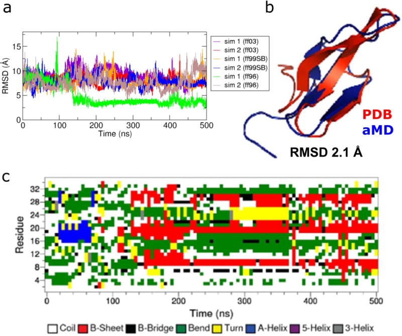
Folding of WW domain simulated via aMD: (a) RMSD plots for the simulations with different AMBER force fields, (b) comparison of simulation-folded WW domain (cyan; blue) with the PDB (2F21) native structure (red) that exhibits 2.1 Å RMSD for the residues between 5 and 30 out of total 35 residues at t = 432 ns, (c) time evolution of the protein secondary structure during the 500 ns simulation run (Run 1) containing the folded structure shown in (b).

Since the simulation of ff96 and (4.0,4.0;0.3,0.3) gives the best result for the protein folding simulation of WW domain, we used these parameters for calculating a two-dimensional PMF profile and we extended the first simulation (sim 1) of ff96 for another 500 ns with the higher frequency (0.2 ps) of saving structures in the trajectory. In this extended simulation, we observed an unfolding event, in which the RMSD increases with time (see Fig. S10a). However, because of insufficient sampling, the error is substantially propagated during the reweighting of the aMD simulation, leading to large noise in the reweighted PMF. Nonetheless, we included the non-reweighted PMF profile (Fig. S10b) for qualitative comparison with the Anton simulation result (see Fig. S6d). Other than the folded state, the two PMF profiles exhibit another similar conformational state near R_g = ~8 Å, although the corresponding RMSD values are different. Note that the energy barrier between the two conformational states observed in aMD non-reweighted PMF is significantly lower than that of the Anton cMD simulation.

The time evolution of the protein secondary structure during the 500 ns aMD simulation containing the native structure shown in Fig. 4a is plotted in Fig. 4c (see Fig. S11 for data of all four independent aMD simulations). Initially, WW domain shows bend secondary structures but when RMSD is significantly reduced at ~ 150 ns, three-stranded β sheet emerges and then WW domain maintains the β-sheet structure for the rest of simulation time, with low RMSD values. However, we noticed that when it is in unfolded states, WW domain can have various secondary structure motifs including α helix. (see Fig. S11). In fact, the observation of helical states was also reported in a microsecond simulation of WW domain with CHARMM22 force field¹².

Discussion

In the present study, extensive aMD simulations captured the folding of four fast-folding proteins that exhibit different secondary structures, including the β-hairpin or turn (chignolin), α-helix (Trp-cage and villin) and β-sheet (WW domain). Notably, the improved reweighting of aMD simulations using cumulant expansion to the 2^nd order provides a remarkable quantitative picture of the folding thermodynamics in both chignolin and Trp-cage while a reasonable quantitative picture is obtained for villin. Despite differences in the simulation force fields (CHARMM22* in the Anton cMD and AMBER ff99SB/ff03/ff14SB in aMD) and variations in the system preparations (e.g., water box size), the resulting free energy profiles from hundreds-of-nanosecond aMD simulations are comparable to those obtained from cMD simulations that last about three orders of magnitude longer, e.g., 106,000 ns for chignolin, 208,000 ns for Trp-cage, 125,000 ns for villin and 651,000 ns for the WW domain (Fig. S6). Moreover, the free energy profiles allow us to identify intermediate conformations during the protein folding, particularly for Trp-cage and villin. A partially folded intermediate that has a similar radius of gyration as the folded state was found along the folding pathway of Trp-cage. This is consistent with previous experimental UV resonance Raman spectroscopy⁶³, infrared spectroscopy⁶⁴ and NMR⁶⁵ studies. For villin, the presence of an intermediate has also been confirmed using triplet-triplet-energy transfer experiments66 and validated by molecular dynamics simulations and Markov state models67.

For chignolin, the aMD simulations identified both the folded and unfolded states from the 2D (RMSD, R_g) PMF profile centered at (0.5 Å, 4.0 Å) and (4.0 Å, 5.5 Å), respectively. In Anton cMD simulation of chignolin, while the unfolded state exhibits lower free energy (~2.0 kcal/mol) and significantly broader energy well, the folded state is found at similar position as the global energy minimum. Furthermore, the folding energy barrier of chignolin is similar in aMD (~3.5 kcal/mol) and cMD (~3.0 kcal/mol) simulations.

For Trp-cage, three distinct folded, intermediate and unfolded states are identified from PMF profile of the aMD simulation. In comparison, while similar folded and intermediate states were found in the Anton cMD simulation, the fully unfolded (extended) state was absent due to the small size of a cubic water box of ~37 Å side length containing ~1,700 water molecules⁷ compared with 11,355 waters used in the present aMD simulation. However, the intermediate state exhibits a similar low-energy well that is centered at (5.0 Å, 7.5 Å) and (5.0 Å, 8.0 Å) in the aMD and Anton cMD simulations, respectively. Moreover, the transition energy barrier between the intermediate and folded states is also similar in aMD (~1.5 kcal/mol) and cMD (~2.0 kcal/mol) simulations.

For villin, folding and unfolding of both wild-type and norleucine double mutant have been extensively discussed and a vast amount of information on the folding mechanism is available in the literature.^68,69 Earlier experimental and computational studies showed that the double mutant folds five times faster than the wild-type form. Piana and coworkers determined a folding time of 19 μs to wild-type villin while the folding time of the double mutant is roughly 3 μs.⁶⁸ Here, we demonstrate that aMD is able to capture folding of the wild-type villin (PDB code 1YRF) during 500–1,500 ns simulations. We have systematically simulated villin folding using a broad range of parameters in order to identify the most appropriate ones to reproduce the native state. It is clear that a different set of parameters will be required to efficiently study distinct biomolecular transitions of folded proteins or to simulate protein folding starting from an extended conformation. Our results show that finding the proper parameters is of capital importance for protein folding studies using aMD. A significant increase of the total boost parameters b₁ and b₂ was required to achieve folding in an affordable simulation time. For villin, the best parameter sets were (4.0,4.0;0.3,0.3), (3.5.3.5;0.3,0.3), and (4.0,4.0;0.25,0.25). A number of folding events were observed in less than 200 ns of aMD simulations providing RMSD values lower than 1 Å with respect to the experimental structure. Our results point out the importance of increasing the total boost parameters while dihedral boost seems to play a less important role. The main conclusion that can be extracted from this part is that through the fine-tuning of aMD parameters one can accelerate the identification of folded states of a protein while keeping the atomistic description of the system. These results suggest that a set of parameters that significantly enhance protein folding can be identified for each system. Our criterion to select the most appropriate set of aMD parameters for villin simulations was to systematically increase the total boost parameter until a folding event was observed in less than 200 ns of aMD simulation. However, there is not a unique approach to identify the most suitable aMD parameters and different strategies can be followed depending on the characteristic features of the studied system (e.g., size, shape and secondary structures). Therefore, it is important to note that the parameter set that we selected for the final simulations of villin may not be the best choice, but it rather serves as a good starting point for other protein folding studies. A detailed analysis is recommended for each particular system. This work paves the way towards an individualized parameter selection as a tool to study protein folding. Here we have only tuned α and E within the dual-boost framework, however, other versions of aMD could be considered. For example, the adaptive accelerated molecular dynamics method may represent an attractive alternative to dual-boost aMD since parameters are optimized along the aMD trajectory depending on the features of the potential energy landscape⁷⁰. We hope that these results will provide guidelines for future studies of aMD on protein folding.

Although they are not directly comparable, the two-dimensional PMF built for wild-type villin headpiece agrees qualitatively with that of the norleucine double mutant obtained from Anton cMD simulations. The PMF profile of the aMD simulations clearly identifies folded, intermediate and unfolded states using both AMBER ff03 and ff14SB force fields giving similar structures for each state. In general, ff14SB samples a larger conformational space compared to ff03 and the shape of the PMF and the position of the critical points becomes similar to what is observed in Anton cMD simulations of the norleucine double-mutant. Interestingly, in 4.5 μs of aMD simulations we explored a similar conformational space as 125 μs of cMD. In addition, in 1.5 μs of independent aMD simulation we were able to capture more than one folding and unfolding event clearly indicating a considerable speed up with respect to the predicted folding time of 19 μs. Finally, significant differences were observed for the energy barriers computed between the folded and intermediate states of ff03 and ff14SB simulations. Note that larger errors are normally found for the energy barriers than in the low energy wells, due to limited number of simulation frames saved in the high-energy regions. Thus aMD suffers from higher energetic noise (less sampling) during reweighting of the energy barriers.

For WW domain, folding from the unfolded to the folded state was observed in aMD simulations using the ff96 force field and the best aMD parameter set selected from villin simulations. Apparently, aMD simulation is also dependent on force field as in cMD simulation, and as a result, we could not observe protein folding in the simulation with ff03 force field, which is consistent with the same result in cMD simulation.¹⁴ Therefore, it is important to use accurate force field in aMD simulations as well. Along with the discussion above, the aMD parameter set optimized for villin (α-helical structure) may not be the best for WW domain (β-sheet structures), but we demonstrated that this parameter set successfully accelerates protein folding process. One may use this working parameter set as a starting point in search for the better parameter sets, as we did for villin. In contrast to the other three proteins, we did not calculate the reweighted free energy profile for WW domain because of insufficient sampling in the folding-unfolding event but provided the non-reweighted free energy profile obtained from the aMD simulation. Nevertheless, the overall shapes of PMFs between our non-reweighted aMD result and the Anton result are similar. To improve, it is necessary to sufficiently sample states and this can be done by finding good aMD parameters producing multiple folding and unfolding events, and with those parameters, by performing multiple independent simulations. Then, one can construct reweighted free energy profiles as we did for the three proteins, which enable one to find intermediate states, and calculate the energy barriers between the states, and finally reveal the folding pathway. This could be addressed separately in future study.

For larger proteins (villin and WW domain), we used more aggressive aMD acceleration parameters compared to smaller proteins (chignolin and Trp-cage). This suggests that as the size of protein increases, the system visits larger accessible conformation space with greater entropic effects (e.g., more possible intermediate states and deeper local free-energy minima) and higher acceleration is required for efficient sampling on the more complex free energy landscapes. In order to escape from the deeper energy minima, strong perturbation with greater aMD acceleration is necessary. This is distinct from typical aMD simulations using relatively weak perturbation for studying the dynamics of proteins near equilibrium states. Generally speaking, reweighting becomes more challenging for larger systems that require higher boost potentials for enhanced sampling. Nevertheless, once the boost potential follows Gaussian distribution with small enough standard deviation, reweighting using cumulant expansion to the 2^nd order could be accurate³⁹. Future studies are aimed at constructing such boost potential for accurate reweighting of aMD simulations on large proteins.

In conclusion, we showed that aMD provides a significant speed up with respect to cMD in protein-folding simulations, and our study of the four fast-folding proteins will be a useful guidance in conducting similar types of protein-folding study. However, speed up of aMD with respect to cMD simulations can be dependent on the system parameters such as the size of the system, simulation temperature, and force field. Therefore, exploring aMD parameter space is recommended in order to achieve optimal acceleration for conformational sampling.

References

- 1.Lane TJ, Shukla D, Beauchamp KA, Pande VS. Curr Opin Struct Biol. 2013;23(1):58–65. doi: 10.1016/j.sbi.2012.11.002. [DOI] [PMC free article] [PubMed] [Google Scholar]
- 2.Piana S, Klepeis JL, Shaw DE. Curr Opin Struct Biol. 2014;24:98–105. doi: 10.1016/j.sbi.2013.12.006. [DOI] [PubMed] [Google Scholar]
- 3.Zhu X, Lopes PEM, MacKerell AD. Wiley Interdisciplinary Reviews-Computational Molecular Science. 2012;2(1):167–185. doi: 10.1002/wcms.74. [DOI] [PMC free article] [PubMed] [Google Scholar]
- 4.Case DA, D TA, Cheatham TE, III, Simmerling CL, Wang J, Duke RE, Luo R, Walker RC, Zhang W, Merz KM, Roberts B, Hayik S, Roitberg A, Seabra G, Swails J, Goetz AW, Kolossváry I, Wong KF, Paesani F, Vanicek J, Wolf RM, Liu J, Wu X, Brozell SR, Steinbrecher T, Gohlke H, Cai Q, Ye X, Wang J, Hsieh M-J, Cui G, Roe DR, Mathews DH, Seetin MG, Salomon-Ferrer R, Sagui C, Babin V, Luchko T, Gusarov S, Kovalenko A, Kollman PA. University of California, San Francisco. 2012 [Google Scholar]
- 5.Kaminski GA, Friesner RA, Tirado-Rives J, Jorgensen WL. J Phys Chem B. 2001;105(28):6474–6487. [Google Scholar]
- 6.Schmid N, Christ CD, Christen M, Eichenberger AP, van Gunsteren WF. Comput Phys Commun. 2012;183(4):890–903. [Google Scholar]
- 7.Lindorff-Larsen K, Piana S, Dror RO, Shaw D. Science. 2011;334(6055):517–520. doi: 10.1126/science.1208351. [DOI] [PubMed] [Google Scholar]
- 8.Satoh D, Shimizu K, Nakamura S, Terada T. FEBS Lett. 2006;580(14):3422–3426. doi: 10.1016/j.febslet.2006.05.015. [DOI] [PubMed] [Google Scholar]
- 9.Enemark S, Kurniawan NA, Rajagopalan R. Scientific Reports. 2012;2 doi: 10.1038/srep00649. [DOI] [PMC free article] [PubMed] [Google Scholar]
- 10.Freddolino PL, Schulten K. Biophys J. 2009;97(8):2338–2347. doi: 10.1016/j.bpj.2009.08.012. [DOI] [PMC free article] [PubMed] [Google Scholar]
- 11.Piana S, Lindorff-Larsen K, Shaw DE. Proc Natl Acad Sci U S A. 2013;110(15):5915–5920. doi: 10.1073/pnas.1218321110. [DOI] [PMC free article] [PubMed] [Google Scholar]
- 12.Freddolino PL, Liu F, Gruebele M, Schulten K. Biophysical journal. 2008;94(10):L75–L77. doi: 10.1529/biophysj.108.131565. [DOI] [PMC free article] [PubMed] [Google Scholar]
- 13.Piana S, Lindorff-Larsen K, Shaw DE. Biophysical journal. 2011;100(9):L47–L49. doi: 10.1016/j.bpj.2011.03.051. [DOI] [PMC free article] [PubMed] [Google Scholar]
- 14.Lindorff-Larsen K, Maragakis P, Piana S, Eastwood MP, Dror RO, Shaw DE. PLoS ONE. 2012;7(2):e32131. doi: 10.1371/journal.pone.0032131. [DOI] [PMC free article] [PubMed] [Google Scholar]
- 15.Huang W, Lin Z, van Gunsteren WF. Journal of Chemical Theory and Computation. 2011;7(5):1237–1243. doi: 10.1021/ct100747y. [DOI] [PubMed] [Google Scholar]
- 16.Ensign DL, Pande VS. Biophysical Journal. 2009;96(8):L53–L55. doi: 10.1016/j.bpj.2009.01.024. [DOI] [PMC free article] [PubMed] [Google Scholar]
- 17.Nguyen H, Maier J, Huang H, Perrone V, Simmerling C. Journal of the American Chemical Society. 2014;136(40):13959–13962. doi: 10.1021/ja5032776. [DOI] [PMC free article] [PubMed] [Google Scholar]
- 18.Mittal J, Best RB. Biophys J. 2010;99(3):L26–L28. doi: 10.1016/j.bpj.2010.05.005. [DOI] [PMC free article] [PubMed] [Google Scholar]
- 19.Cino EA, Choy WY, Karttunen M. J Chem Theory Comput. 2012;8(8):2725–2740. doi: 10.1021/ct300323g. [DOI] [PMC free article] [PubMed] [Google Scholar]
- 20.Kührová P, De Simone A, Otyepka M, Best RB. Biophysical journal. 2012;102(8):1897–1906. doi: 10.1016/j.bpj.2012.03.024. [DOI] [PMC free article] [PubMed] [Google Scholar]
- 21.Best RB, Hummer G. The Journal of Physical Chemistry B. 2009;113(26):9004–9015. doi: 10.1021/jp901540t. [DOI] [PMC free article] [PubMed] [Google Scholar]
- 22.Zhou R, Maisuradze GG, Suñol D, Todorovski T, Macias MJ, Xiao Y, Scheraga HA, Czaplewski C, Liwo A. Proceedings of the National Academy of Sciences. 2014;111(51):18243–18248. doi: 10.1073/pnas.1420914111. [DOI] [PMC free article] [PubMed] [Google Scholar]
- 23.Sugita Y, Okamoto Y. Chem Phys Lett. 1999;314(1–2):141–151. [Google Scholar]
- 24.Deng N-j, Dai W, Levy RM. The Journal of Physical Chemistry B. 2013 doi: 10.1021/jp401962k. [DOI] [PMC free article] [PubMed] [Google Scholar]
- 25.Marinelli F, Pietrucci F, Laio A, Piana S. PLoS Comput Biol. 2009;5(8) doi: 10.1371/journal.pcbi.1000452. [DOI] [PMC free article] [PubMed] [Google Scholar]
- 26.Juraszek J, Bolhuis PG. Proc Natl Acad Sci U S A. 2006;103(43):15859–15864. doi: 10.1073/pnas.0606692103. [DOI] [PMC free article] [PubMed] [Google Scholar]
- 27.Deng N-j, Dai W, Levy RM. The Journal of Physical Chemistry B. 2013;117(42):12787–12799. doi: 10.1021/jp401962k. [DOI] [PMC free article] [PubMed] [Google Scholar]
- 28.Granata D, Camilloni C, Vendruscolo M, Laio A. Proceedings of the National Academy of Sciences. 2013;110(17):6817–6822. doi: 10.1073/pnas.1218350110. [DOI] [PMC free article] [PubMed] [Google Scholar]
- 29.Hamelberg D, Mongan J, McCammon JA. J Chem Phys. 2004;120(24):11919–11929. doi: 10.1063/1.1755656. [DOI] [PubMed] [Google Scholar]
- 30.Hamelberg D, de Oliveira CAF, McCammon JA. J Chem Phys. 2007;127(15):155102. doi: 10.1063/1.2789432. [DOI] [PubMed] [Google Scholar]
- 31.Wereszczynski J, McCammon JA. Proc Natl Acad Sci U S A. 2012;109(20):7759–7764. doi: 10.1073/pnas.1117441109. [DOI] [PMC free article] [PubMed] [Google Scholar]
- 32.Gasper PM, Fuglestad B, Komives EA, Markwick PRL, McCammon JA. Proc Natl Acad Sci U S A. 2012;109(52):21216–21222. doi: 10.1073/pnas.1218414109. [DOI] [PMC free article] [PubMed] [Google Scholar]
- 33.Pierce LCT, Markwick PRL, McCammon JA, Doltsinis NL. J Chem Phys. 2011;134(17) doi: 10.1063/1.3581093. [DOI] [PMC free article] [PubMed] [Google Scholar]
- 34.Bucher D, Grant BJ, Markwick PR, McCammon JA. PLoS Comput Biol. 2011;7(4):e1002034. doi: 10.1371/journal.pcbi.1002034. [DOI] [PMC free article] [PubMed] [Google Scholar]
- 35.Wang Y, Markwick PRL, de Oliveira CAF, McCammon JA. J Chem Theory Comput. 2011;7(10):3199–3207. doi: 10.1021/ct200430c. [DOI] [PMC free article] [PubMed] [Google Scholar]
- 36.Pierce LCT, Salomon-Ferrer R, de Oliveira CAF, McCammon JA, Walker RC. J Chem Theory Comput. 2012;8(9):2997–3002. doi: 10.1021/ct300284c. [DOI] [PMC free article] [PubMed] [Google Scholar]
- 37.Miao Y, Nichols SE, Gasper PM, Metzger VT, McCammon JA. Proc Natl Acad Sci U S A. 2013;110(27):10982–10987. doi: 10.1073/pnas.1309755110. [DOI] [PMC free article] [PubMed] [Google Scholar]
- 38.Doshi U, Hamelberg D. The Journal of Physical Chemistry Letters. 2014;5(7):1217–1224. doi: 10.1021/jz500179a. [DOI] [PubMed] [Google Scholar]
- 39.Miao Y, Sinko W, Pierce L, Bucher D, McCammon JA. J Chem Theory Comput. 2014;10(7):2677–2689. doi: 10.1021/ct500090q. [DOI] [PMC free article] [PubMed] [Google Scholar]
- 40.Markwick PRL, McCammon JA. Phys Chem Chem Phys. 2011;13(45):20053–20065. doi: 10.1039/c1cp22100k. [DOI] [PubMed] [Google Scholar]
- 41.Doshi U, Hamelberg D. Journal of Chemical Theory and Computation. 2012;8(11):4004–4012. doi: 10.1021/ct3004194. [DOI] [PubMed] [Google Scholar]
- 42.Shen TY, Hamelberg D. J Chem Phys. 2008;129(3):034103. doi: 10.1063/1.2944250. [DOI] [PubMed] [Google Scholar]
- 43.Hummer G. J Chem Phys. 2001;114(17):7330–7337. [Google Scholar]
- 44.Eastwood MP, Hardin C, Luthey-Schulten Z, Wolynes PG. J Chem Phys. 2002;117(9):4602–4615. [Google Scholar]
- 45.Sinko W, Miao Y, de Oliveira CAF, McCammon JA. J Phys Chem B. 2013;117(42):12759–12768. doi: 10.1021/jp401587e. [DOI] [PMC free article] [PubMed] [Google Scholar]
- 46.Barua B, Lin JC, Williams VD, Kummler P, Neidigh JW, Andersen NH. Protein Eng Des Sel. 2008;21(3):171–185. doi: 10.1093/protein/gzm082. [DOI] [PMC free article] [PubMed] [Google Scholar]
- 47.Chiu TK, Kubelka J, Herbst-Irmer R, Eaton WA, Hofrichter J, Davies DR. Proceedings of the National Academy of Sciences of the United States of America. 2005;102(21):7517–7522. doi: 10.1073/pnas.0502495102. [DOI] [PMC free article] [PubMed] [Google Scholar]
- 48.Jorgensen WL, Chandrasekhar J, Madura JD, Impey RW, Klein ML. J Chem Phys. 1983;79(2):926–935. [Google Scholar]
- 49.Gotz AW, Williamson MJ, Xu D, Poole D, Le Grand S, Walker RC. J Chem Theory Comput. 2012;8(5):1542–1555. doi: 10.1021/ct200909j. [DOI] [PMC free article] [PubMed] [Google Scholar]
- 50.Salomon-Ferrer R, Götz AW, Poole D, Le Grand S, Walker RC. J Chem Theory Comput. 2013;9(9):3878–3888. doi: 10.1021/ct400314y. [DOI] [PubMed] [Google Scholar]
- 51.Salomon-Ferrer R, Case DA, Walker RC. Wiley Interdisciplinary Reviews-Computational Molecular Science. 2013;3(2):198–210. [Google Scholar]
- 52.Le Grand S, Gotz AW, Walker RC. Comput Phys Commun. 2013;184(2):374–380. [Google Scholar]
- 53.Ensign DL, Kasson PM, Pande VS. Journal of Molecular Biology. 2007;374(3):806–816. doi: 10.1016/j.jmb.2007.09.069. [DOI] [PMC free article] [PubMed] [Google Scholar]
- 54.Best RB. Curr Opin Struct Biol. 2012;22(1):52–61. doi: 10.1016/j.sbi.2011.12.001. [DOI] [PubMed] [Google Scholar]
- 55.Wang T, Wade RC. Journal of Chemical Theory and Computation. 2006;2(1):140–148. doi: 10.1021/ct0501607. [DOI] [PubMed] [Google Scholar]
- 56.Jager M, Zhang Y, Bieschke J, Nguyen H, Dendle M, Bowman ME, Noel JP, Gruebele M, Kelly JW. Proceedings of the National Academy of Sciences of the United States of America. 2006;103(28):10648–10653. doi: 10.1073/pnas.0600511103. [DOI] [PMC free article] [PubMed] [Google Scholar]
- 57.Ryckaert J-p, Ciccotti G, Berendsen HJC. J Comput Phys. 1977;23(3):327–341. [Google Scholar]
- 58.Berendsen HJC, Postma JPM, Vangunsteren WF, Dinola A, Haak JR. J Chem Phys. 1984;81(8):3684–3690. [Google Scholar]
- 59.Essmann U, Perera L, Berkowitz ML, Darden T, Lee H, Pedersen LG. J Chem Phys. 1995;103(19):8577–8593. [Google Scholar]
- 60.Humphrey W, Dalke A, Schulten K. Journal of molecular graphics. 1996;14(1):33–38. doi: 10.1016/0263-7855(96)00018-5. [DOI] [PubMed] [Google Scholar]
- 61.Hess B, Kutzner C, van der Spoel D, Lindahl E. J Chem Theory Comput. 2008;4(3):435–447. doi: 10.1021/ct700301q. [DOI] [PubMed] [Google Scholar]
- 62.Harada R, Kitao A. Journal of Chemical Theory and Computation. 2011;8(1):290–299. doi: 10.1021/ct200363h. [DOI] [PubMed] [Google Scholar]
- 63.Ahmed Z, Beta IA, Mikhonin AV, Asher SA. J Am Chem Soc. 2005;127(31):10943–10950. doi: 10.1021/ja050664e. [DOI] [PubMed] [Google Scholar]
- 64.Meuzelaar H, Marino KA, Huerta-Viga A, Panman MR, Smeenk LEJ, Kettelarij AJ, van Maarseveen JH, Timmerman P, Bolhuis PG, Woutersen S. J Phys Chem B. 2013;117(39):11490–11501. doi: 10.1021/jp404714c. [DOI] [PubMed] [Google Scholar]
- 65.Rovo P, Straner P, Lang A, Bartha I, Huszar K, Nyitray L, Perczel A. Chemistry-a European Journal. 2013;19(8):2628–2640. doi: 10.1002/chem.201203764. [DOI] [PubMed] [Google Scholar]
- 66.Reiner A, Henklein P, Kiefhaber T. Proc Natl Acad Sci U S A. 2010;107(11):4955–4960. doi: 10.1073/pnas.0910001107. [DOI] [PMC free article] [PubMed] [Google Scholar]
- 67.Beauchamp KA, Ensign DL, Das R, Pande VS. Proc Natl Acad Sci U S A. 2011;108(31):12734–12739. doi: 10.1073/pnas.1010880108. [DOI] [PMC free article] [PubMed] [Google Scholar]
- 68.Piana S, Lindorff-Larsen K, Shaw DE. Proceedings of the National Academy of Sciences. 2012;109(44):17845–17850. doi: 10.1073/pnas.1201811109. [DOI] [PMC free article] [PubMed] [Google Scholar]
- 69.Banushkina PV, Krivov SV. Journal of Chemical Theory and Computation. 2013;9(12):5257–5266. doi: 10.1021/ct400651z. [DOI] [PMC free article] [PubMed] [Google Scholar]
- 70.Markwick PRL, Pierce LCT, Goodin DB, McCammon JA. J Phys Chem Lett. 2011;2(3):158–164. doi: 10.1021/jz101462n. [DOI] [PMC free article] [PubMed] [Google Scholar]
Associated Data
This section collects any data citations, data availability statements, or supplementary materials included in this article.