Human Linear Growth Trajectory Defined

Abstract

Objectives

The purpose of this study was to assess the applicability of a simple mathematical formula for prediction of individual child linear growth. The formula describes a square root dependence of height on age with only two constants, k and C.

Methods

Retrospective serial height measurements of 137 healthy children (61 female), who attended clinic in the Pediatrics Department at the University of California, San Francisco were used. For each child, two of the initial measurements and their corresponding measurement times were used to determine the values of k and C. By substituting the determined values of k and C into the formula, the formula was then used to predict the trajectory of the child’s growth.

Results

The 137 children were comprised of 20% Hispanic, 23% African-American, 27% Caucasian and 30% Asian. The formula predicted growth trajectories of 136 out of the 137 children with minimal discrepancies between the measured data and the corresponding predicted data. The mean of the discrepancies was 0.8 cm.

Conclusions

Our proposed formula is very easy to use and predicts individual child growth with high precision irrespective of gender or ethnicity. The formula will be a valuable tool for studying human growth and possibly growths of other animals.

Animals and human growth trajectories have been of immense interest to scientists for decades. As such, several mathematical models have been suggested for fitting growth trajectories (for review see Karkach, 2006; Katsunori, 2006; Preece and Heinrich, 1981; Zotina and Zotina, 1972). A common feature of these models is that they contain several parameters and achieve good fit to growth data only through statistical optimization of the parameters. Even with parameter optimization only a few of the models are able to fit the human growth curve from birth to adulthood, because of its complexity (see Preece and Heinrich, 1981). Thus to date a theoretically derived non-parametric mathematical formula that precisely defines human and/or other animal growth is nonexistent.

Recently, we proposed and validated a mathematical formula that describes human brain tissue volume regrowth (recovery) in abstinent alcohol dependent adults (Mon et al., 2011). The pattern of human brain tissue volume recovery in this population is similar to the pattern of observed child growth. Specifically, brain tissue volume gain in abstinent alcohol dependent individuals decreases with duration of abstinence (Gazdzinski et al., 2005; Pfefferbaum et al., 1995) just as gain in height of a child decreases with age, as documented for some portions of the human growth trajectory (see Karlberg et al., 1994). This suggests that growth rate of a child has an inverse relation with age. Indeed, Schmalhausen studied growth of animals based on the assumption that growth rate depends inversely on time (see Birnholz, 1980). Because height (or size) of a normal growing child is directly proportional to time (age), it implies that growth rate also has an inverse relation with height. On the basis of the foregoing arguments, we posited that our mathematical formula, which describes brain tissue volume recovery of abstinent alcohol dependent individuals, also describes the trajectory of human growth. The formula describes a square root dependence of growth on age. As human linear growth consists of portions (segments); we hypothesized that our mathematical formula accurately describes each individual segment of the entire growth, hence describing the entire trajectory of human growth.

METHODS

Brief description of the formula

Below we give a brief description of the human growth version of the original formula proposed for prediction of brain tissue volume recovery in abstinent alcohol dependent individuals (Mon et al., 2011).

Suppose the height (H) of a child at time (t) is H_(t) and that at a later time (t+τ) is H_(t+τ). Let the magnitude of the rate of increase $\left(\frac{dH}{dt}\right)$ of H at t be A_(t) and that at t+τ be A_(t+τ). In normal uninterrupted growth (at least within a given segment of the human growth), H_(t+τ) > H_(t), but A_(t+τ) < A_(t). For example, a child’s height in its 3rd year of age is greater than that in the 2nd year, but its growth rate in the 3rd year is slower than that in the 2nd year. This pattern of growth suggests an inverse dependence of growth rate on height: i.e.,

$$\frac{dH}{dt}\propto \frac{1}{H}\text{or}\frac{dH}{dt}=\frac{k}{H}$$ (1)

where k is a constant of proportionality unique to the individual. Here we refer to k as the growth rate factor (or growth coefficient) of the child and it is influenced by factors such as genetics, gender, environment, general medical and psychiatric condition and other unknown factors. It is important to note that the purpose of this study was not to determine how much each of the factors mentioned above contributes to the value of k, but rather to determine the overall value of k and input the determined value of k into the formula to predict the child’s growth trajectory.

From Eq. (1) the height of the child at any time can be obtained by integration with respect to t; i.e.,

$$\int \frac{dH}{dt}dt=\int \frac{k}{H}dt\text{or}\int \mathit{HdH}=k\int dt$$ (2)

$$\Rightarrow \frac{1}{2}{H}^2=kt+C$$ (3)

where C is a constant of integration.

If H is known for two different times (t₁) and (t₂), then it follows from Eq. (3) that

$$\begin{array}{l}k=\frac{1}{2(t_2-t_1)}({H_{(t_2)}}^2-{H_{(t_1)}}^2);\text{and}C=\frac{{H_{(t_1)}}^2}{2}-{kt}_1\text{or}\\ C=\frac{{H_{(t_2)}}^2}{2}-{kt}_2\end{array}$$

Therefore, with two height measurements at two different time points, the values of k and C can be estimated and substituted into the formula [Eq. (3)], which can then be used to calculate H for any other time t. If H is measured in centimeters (cm) and time measured in years (yr), the units of C and k are cm² and cm² yr⁻¹ respectively. For better prediction of growth, the interval between the two measurements that are used to estimate C and k must be well separated in time, such that the increment in growth between the two points is greater than measurement error.

Notice that if H₍₀₎ corresponds to t = 0 (an initial time), then Eq. (3) can be written as

$$H^2={H_{(0)}}^2+2kt$$ (4)

Equation (4) is analogous to Newton’s 3rd equation, which describes uniform motion of a body. The only difference is that, whereas Newton’s 3rd equation of motion relates velocity to distance travelled, Eq. (4) of this report relates distance (height) to time. Thus the formula presented in this report describes uniform linear growth of human.

Validation of the formula for prediction of human linear growth trajectory

We tested the formula using retrospective serial height measurements of 137 healthy children (61 female) who attended the pediatrics clinic at the University of California, San Francisco (UCSF) for routine checkups. At each well child visit, height was obtained without footwear and /or headgear and it was measured by a trained medical assistant, a registered nurse or the primary care provider. For children less than 2 years, body length was measured using an infant horizontal stadiometer. For children at 2 years and older, standing height was measured with a standard calibrated stadiometer, with the child standing upright against a backboard to ensure good posture. Typically, a single measurement (to the nearest 0.5 cm) is normally obtained and recorded on a medical chart.

Participants were included in this study if they had more than five serial height measurements entered into their chart following birth. Children with histories of minor medical or psychiatric diagnoses were included in the study. Exclusionary criteria included preterm birth (defined as birth before 36 weeks of gestation) and children with asthma as these conditions are widely known to affect child growth. Also recumbent or standing height measurements that did not have complete dates of measurements were excluded from the analysis.

The trajectory of human growth is made up of specific portions (segments) (see Preece and Heinrick, 1981). These include the infant growth segment (0–2 years), the childhood growth segment (2 years to before the onset of adolescence) and the adolescent growth segment (8—adulthood), which contains the adolescent growth spurt in some children. Because the adolescent growth spurt does not occur in all children, and also because the age of onset of the spurt varies between individual children, to test the accuracy of the formula for predicting growth within each segment (including the growth spurt), all data extending over the adolescence period were first plotted to determine children who experienced growth spurts. Thus generally each child’s data were grouped into infant growth data (0–2 years), childhood growth data (2 + to about 8 years) and adolescent growth data (8+ years). In some children growth did not change during adolescence therefore their data were grouped into 2 segments: from 0 to 2 years and after 2 years. For each child and for each segment the values of k and C were then estimated using any two initial measurements that were separated by at least 4 months and at most 1 year. By substituting the estimated values of k and C into Eq. (3), the formula was then used to predict other measurements of the child’s growth. For instance, if k = 700 cm² yr⁻¹ and C = 1,700 cm² for a given segment of a child, then the equation of growth of the child for the segment was $\frac{1}{2}{H}^2=700t+1700$; from which H was predicted for the rest of the measurements of the segment’s trajectory.

The predicted data were then compared with the measured data using three statistical procedures: (i) calculation of differences between measured and predicted data to assess the accuracy of the formula in predicting individual child growth, (ii) performing intraclass correlation analyses to assess the degree of similarity between the measured and predicted data, and (iii) performing paired t tests between the measured and predicted data to assess the statistical similarities (or otherwise) between the means of the two sets of data. All segmental curves obtained with the formula for each child were also plotted on the same axes, which then merged to form a complete linear growth trajectory of the child. The measured data were then plotted on the same axes with the corresponding predicted curves for visualization and comparison. We also compared the performance of our formula with the performances of Preece–Baines and the Triple Logistic models by fitting the models to growth data of one of the participants (a girl) with uniform growth data between 2 and 12 years.

This research met conditions for involvement of children (45 CFR 46.404, 21 CFR 50.51) and neonates (45 CFR 46.205) for research and was approved with waiver on inform consent by the Committee on Human Research of the University of California, San Francisco. The requirement for individual HIPAA authorization was also waived for all subjects.

RESULTS

Demographics summary

The participants were racially/ethnically diverse, based on parents report. Initially, serial height measurements of 164 (69 female) children were extracted from their medical records. Twenty of the children (five girls) were born premature (premature birth is defined as birth before 36 weeks of gestation) and seven (three girls) were diagnosed with asthma; data of these children were excluded from the analysis. These exclusions reduced the sample to 137 children, which was then analyzed and used for this report. The analyzed sample comprised of 27 Hispanic (15 female), 32 African-American (15 female), 37 Caucasian (14 female), and 41 Asian (17 female). Five participants (all girls) were diagnosed with obesity, 3 (1 girl) with scoliosis, and 2 (both boys) with pharyngitis during the periods of their visits to the pediatric department at UCSF. There was also 1 case each of pancreatitis (boy), conjunctivitis (boy), Hashimoto’s thyroiditis (boy) and breast hypertrophy (girl). About 31% of the participants had data from birth to about 2-years old, 36% had data from birth to over 2 years and 33% had data from 2 years or after 2 years old. Table 1 shows the data distribution of the sample across ethnicity and age of the participants. Fifty three of the children had measurements through the age range of the adolescent growth spurt; of which 28 showed increase in growth rate (adolescent growth/growth spurt) during this range.

TABLE 1.

Demographics and distribution of height measurements

Variable	AAM no.	AAF no.	ASM no.	ASF no.	CAM no.	CAF no.	HPM no.	HPF no.
0–2 yr data.	6	4	7	5	4	3	7	6
0–2 +yr data	6	3	9	3	17	4	4	3
2 +yr data	5	8	8	9	2	7	1	6

AAM = African-American male; AAF = African-American female; ASM = Asian male; ASF = Asian female; CAM = Caucasian male; CAF = Caucasian female; HPM = Hispanic male; HPF = Hispanic female; No. = number of cases.

Percentage differences between measured and predicted data

Figure 1 shows the deviations of the predicted individual height measurements (estimated as predicted height minus measured height, in cm) plotted against age of prediction for 32 selected children with 395 data points covering a wide range of the growth trajectory. The line H = 0 denotes zero deviation of predicted height values from measured height values. As seen for these children, the deviations of the formula predictions are randomly distributed across the entire growth period. To further illustrate the accuracy of the formula in predicting child linear growth across all ages, Table 2 shows four randomly selected pairs of the measured and predicted data for 25 randomly selected children, but equal gender distribution. The distribution of the data points in the table ranged from birth to late adolescence but because of space limitation the corresponding ages are not included in the table. The columns labeled H_me show the measured height values, while those labeled H_pr show the corresponding predicted data. The ΔH columns show the discrepancies (H_pr − H_me) between each preceding set of H_me and H_pr values, while ΔH_in shows the means of the absolute values of ΔH of each child. ΔH_in ranged from 0.1 to 2.1 cm with a mean value of 0.9 cm for the data presented in Table 2. Similar results were obtained for the entire sample of children; ΔH_in ranged from 0.1 to 2.8 cm with a mean of 0.9 cm, demonstrating good prediction. Importantly, ΔH for each child fluctuated between negative and positive values about the measured data, demonstrating that the discrepancies observed were not systematic errors from the formula. Also the discrepancies were very similar irrespective of age, gender or ethnicity. However larger discrepancies (4–9 cm) were observed in some portions of the curves of one obese child and two scoliosis diagnosed children (data not shown here).

Fig. 1.

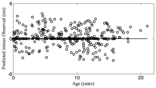
Plot of deviation of formula prediction of individual child growth from actual measurements against age of prediction.

TABLE 2.

Measured height (H_me), predicted height (H_pr) and discrepancy (ΔH) between H_me and H_pr for 25 children (12 females)

Child	Hme (cm)	Hpr (cm)	ΔH (cm)	Hme (cm)	Hpr (cm)	ΔH (cm)	Hme (cm)	Hpr (cm)	ΔH (cm)	Hme (cm)	Hpr (cm)	ΔH (cm)	ΔHin (cm)
1	124.5	124.9	0.4	129.5	129.5	0.0	148.6	146.8	−1.8	139.7	137.7	−2.0	1.1 ± 1.0
2	90.2	89.2	−1.0	127.0	126.7	−0.3	138.4	138.7	0.3	150.1	151.3	1.2	0.7 ± 0.5
3	99.8	99.3	−0.5	127.8	127.5	−0.3	134.6	134.9	0.3	139.2	143.5	4.3	1.4 ± 2.0
4	102.4	102.4	0.0	131.5	131.3	−0.2	138.4	138.2	−0.2	157.5	157.5	0.0	0.1 ± 0.1
5	127.0	127.8	0.8	139.2	136.9	−2.3	141.7	141.2	−0.5	143.0	143.3	0.3	1.0 ± 0.9
6	121.9	120.7	−1.2	135.9	135.4	−0.5	141.0	140.2	−0.8	144.3	144.3	0.0	0.4 ± 0.8
7	120.7	120.4	−0.3	131.6	131.8	0.2	137.4	137.2	−0.2	143.0	142.5	−0.5	0.3 ± 0.1
8	67.3	65.3	−2.0	80.0	81.0	1.0	85.1	85.6	0.5	89.7	89.4	−0.3	1.0 ± 0.8
9	27.5	28.0	0.5	31.5	31.4	−0.1	36.5	36.6	0.1	41.2	41.2	0.0	0.2 ± 0.2
10	32.5	31.9	−0.6	42.0	41.7	−0.3	44.3	44.0	−0.3	48.0	48.0	0.0	0.3 ± 0.2
11	25.7	25.9	0.2	31.0	30.7	−0.3	33.8	33.4	−0.4	37.0	36.9	−0.1	0.3 ± 0.1
12	27.3	27.5	0.2	39.8	39.4	−0.4	42.5	42.1	−0.4	45.0	45.7	0.7	0.4 ± 0.2
13	98.3	98.8	0.5	120.7	120.4	−0.3	127.0	127.3	0.3	137.4	137.2	−0.2	0.3 ± 0.1
14	69.3	70.1	0.8	85.1	86.4	1.3	89.7	90.2	0.5	106.7	106.7	0.0	0.7 ± 0.5
15	101.6	103.9	2.3	126.0	125.2	−0.8	140.5	141.2	0.7	153.7	155.2	1.5	1.3 ± 0.7
16	159.3	158.8	−0.5	159.0	159.3	0.3	158.2	159.4	3.0	160.3	159.8	−0.5	1.1 ± 1.3
17	128.5	129.5	1.0	154.9	153.9	−1.0	158.8	160.0	1.2	162.3	163.6	1.3	1.1 ± 0.2
18	54.6	55.4	0.8	63.5	63.0	−0.5	65.5	66.8	1.3	88.4	87.9	1.5	1.0 ± 0.5
19	69.9	69.9	0.0	86.4	87.6	1.2	88.9	90.9	2.0	99.1	100.8	1.7	1.2 ± 0.9
20	146.1	146.6	0.5	160.0	157.8	−2.2	168.9	166.6	−2.3	175.3	178.6	3.3	2.1 ± 1.2
21	95.8	92.7	−3.1	122.7	123.2	0.5	137.9	138.2	0.3	155.7	156.2	0.5	1.1 ± 1.3
22	64.5	64.5	0.0	74.9	76.5	1.6	82.0	83.6	1.6	122.7	123.2	0.5	0.9 ± 0.8
23	59.7	58.4	−1.3	68.6	71.1	2.5	97.8	97.6	−0.2	100.3	101.1	0.8	1.2 ± 1.0
24	67.1	66.5	−0.6	78.7	80.5	1.8	85.9	87.4	1.5	103.6	107.9	4.3	2.1 ± 1.6
25	74.4	75.4	1.0	95.3	95.5	0.2	96.5	95.8	−0.7	103.6	104.6	1.0	0.7 ± 0.4
Mean ± standard deviation of ΔHin													0.9 ± 0.7

For illustrative purposes, Figure 2 shows plots of the measured height (circular marks) of 8 girls (panel A and B) and 8 boys (panel C and D) with data between birth and at least 12 years old. The solid curves represent our formula description of the individual growths by plotting the individual segments on the same axis. The figure clearly demonstrates that the fits using our formula reflect the individual growth trajectories of the 16 children very well. Similarly accurate fits were obtained for the rest of the children except for one boy who had an inconsistent growth pattern. Figure 3 shows a plot of both the measured data and the formula predicted growth trajectory of this child, using his first two height measurements as inputs to the formula. The reason for the inconsistent growth of this child is not known, because he had no record of a past major medical condition that could have caused an erratic growth pattern. Figure 4 shows fits of our formula (a), the Preece–Baines (b), and the Triple Logistic (c) models to uniform growth data of one of the participants of this cohort. The fit of our formula gave the best root mean square error (RMSE = 0.42), followed by that of the Preece–Baines (RMSE = 0.51); while a NaN value of RMSE was reported by the fitting software for the Triple Logistic model. Fits of other uniform growth data showed similar patterns to the fits in Figure 4.

Fig. 2.

Individual growth data and calculated trajectories for 8 girls (panel A and B) and 8 boys (panel C and D). The circular marks represent the measured height data, while the solid curves represent the individual trajectories obtained from the formula.

Fig. 3.

Growth trajectory of a boy with inconsistent growth. The circular marks represent the measured height data, while the solid curves represent the trajectory prescribed by our formula using any two of the first three height measures to estimate k and C.

Fig. 4.

Comparison of fitting accuracies of three mathematical models: a, Mon’s formula (with RMSE = 0.42); b, Preece—Brained model (with RMSE = 0.51); c, Triple Logistic model (with RMSE = NaN).

Intraclass correlations between measured and predicted data

Intraclass correlation analyses using all measurements of the entire sample yielded an intraclass correlation coefficient of 0.98 between the measured and predicted data. We further divided the data into groups of 0–2 years, 3–6 years, 7–10 years, and 11–18 years and analyzed each group data to see the portion of the growth curve that is best described by the formula. The data for groups 0–2 years, 3–6 years, and 7–10 years each yielded an intraclass correlation coefficient of 0.99, while data for group 11–18 years yielded an intraclass correlation of 0.98. Similar analyses based on gender or ethnicity yielded similar results.

Paired t test between measured and predicted data

Paired t test analyses on the entire data and on each of the subgroups described above (in the intraclass correlation analyses) all gave P values >0.97 (two-tail), indicating high similarities of group means between the measured and predicted height data.

DISCUSSIONS

In this report a simple but novel mathematical formula that describes individual child linear growth is presented. The formula is novel because it uses only two height measurements (at two different times) of an individual child to predict future height values of the child. Table 2 as well as Figures 1, 2, and 4 demonstrates clearly the accuracy of the formula for predicting individual child growth. The intraclass correlation and the paired t test analyses between the measured and predicted data also yielded high intraclass correlation coefficients and p values respectively; further confirming the accuracy of the formula for predicting individual child growth. Importantly, the accuracy of the predictions was not influenced by gender, ethnicity or age of the child after birth. On average the predicted height values were 0.9 cm different from the measured values. This mean discrepancy is not substantially different from the measurement error of 0.5 cm (stated earlier in this report). However, we observed some lager differences between the measured and predicted values (higher predicted values up to 9 cm) that were contiguous over some portions of the growth curve in 1 of the children with obesity and 2 of the children with sciolosis, but we could not conclusively attribute the deviations in growth trajectories of these children to the medical conditions because the medical records did not state the time of occurrence of the conditions.

Our formula is different from and improves upon the existing mathematical models that are used to fit growth data through optimization of several parameters in a number of ways. First, most of the existing models such as those of Gompertz, Nelder, and Preece-Banes (Gompertz, 1825; Nelder, 1961; Preece-Branes, 1978) are developed from exponential functions or a combination of exponential and linear functions (such as Count, 1943; Jens-Baley, 1937). Exponential functions assume that growth rate is directly proportional to height, while linear functions assume that growth rate is constant with age/ height. These two assumptions are contrary to what is observed in child growth. In fact, in an interrupted growth, growth rate generally decreases with height or age and Schmalhausen studied growth of animals based on the assumption that growth rate is inversely proportional to time (see Birnholz, 1980). However, it seems more appropriate to relate growth rate of an individual to their height (rather than time) since height is uniquely influenced by factors such as genetics, environmental and nutritional factors which all influence growth rate. This is the basis of our formula and its accuracy of fit validates our theory that growth rate is inversely proportional to height. For this cohort, our formula gave better data fits for ranges of uniform individual growth data than the Preece–Baines and the triple logistic models, which have been commonly used to fit individual growth data. Also, previous studies of child growth using other growth prediction models on different samples reported larger prediction errors than the errors observed in this report (see Preece and Heinrich, 1981). Another advantage of our formula is that it requires only the values of the growth rate factor (k) and the integration constant (C) as inputs, as opposed to the numerous parameters used in the existing mathematical models that also require laborious statistical optimization methods of curve fitting. However, it is worthy to note that the interval between the two measurements used to calculate k and C in our formula must be well separated in time for accurate estimation of these constants for better height prediction. For this sample the time interval between the two measurements used to estimate k and C for best prediction of other measurements was at least 4 months.

Our formula has several potential applications. For instance, it could be used to predetermine a child’s own growth curve and that curve can then be used as a reference curve for the child. By this way, any future health-related deviations in the child’s growth can easily be detected by plotting measured data against the reference curve; this could be beneficial to physicians in monitoring child growth (at least within a given growth segment). However, for this to be accurate the two measurements used to predict the reference curve must not be abnormal themselves. The normality of the initial measurements may be verified by estimating k twice from two different sets of equally spaced measurements and comparing the values obtained. The possibility of imperfect uniform growth coupled with measurement errors may result in slightly different values of k from the two estimations; however widely varied values of k from the two estimations may signal an abnormality of at least one of the measurements, which may be due to a disease or a normal change in trajectory. Secondly, the formula could be useful in longitudinal research studies of child growth.

Furthermore, our formula was able to predict individual heights up to late adolescence (17 + years) in those children that had complete data from birth or early childhood to late adolescence. However the adolescent growth spurt was treated as a separate segment (adolescent growth: in those children who experienced the phenomenon) for accurate prediction.

The general believe is that the complexity of the human growth curve can only be described through combinations of different multiple functions, each of which describes a specific segment of the curve. However, in this cohort, our formula predicted all the segmental trajectories (including the growth spurt region) of each individual child, except that the value of the growth rate factor (k) and C changed between segments: e.g., for each child the value of the growth rate factor between 2 years of age and the onset of adolescence was about halve the value of the growth rate factor during the first 2 years after birth. Therefore, for this cohort, the complexity of the human growth curve seemed to have originated from the changing value of k, which gives rise to segments with different curvatures. On this note, it is possible that with further research and development a mathematical relation for the growth rate factors of the growth segments could be established, thereby making our formula easily usable in predicting adult stature of a child from infant or earlier childhood data. Currently several mathematical models exist that are used to predict adult stature from a child current growth data (Baley-Pinneau, 1946; Roche et al. 1988; Tanner et al., 1962, 1983). Generally several variables including (but not limited to) the child’s current height, the height at age 2, the current weight, the chronological bone age and the mid-parent height or paternal height are needed as inputs to predict the final height of the child. These requirements render the existing models cumbersome to use. Second the errors associated with the existing models in estimating the adult height are larger (Joss et al., 1992; Limony et at., 1993; Thodberg et al., 2009; Zadik et al., 1996) than those observed in this report. However, a direct comparison of our formula with the existing models using the same sample is needed for a definitive conclusion. Another important point to note is that the trajectories of growth of several other animals have been shown to be similar to that of man (Karkach 2006; Novak et al., 2007). Thus our formula could also be applicable in describing growth of other animals; but this also needs to be tested.

In conclusion, we have used a simple mathematical formula to predict the trajectory of individual human growth. The simplicity of the formula will make it easily usable for studying individual human growth and possibly other animal growth. The formula also has the potential to predict adult human heights of individual children from earlier childhood data (particularly when using adolescent growth data) and could be useful in situations where prediction of future adult height of a child is of interest. Scammon suggested that the pattern of neural growth (e.g., brain growth) is different from growth in stature (see Harris et al., 1930). However, in this report we have predicted individual child linear growth using a mathematical formula that was derived for prediction of human brain regrowth (neural regrowth) during abstinence from chronic abuse of alcohol. The applicability of the formula for prediction of both human linear growth and brain regeneration during abstinence from alcohol dependence suggests that these two processes share the same trajectory, but with different growth rates. However, it remains to be tested if the growths of other human body parts also follow the same trajectory.

LITERATURE CITED

- Baley N. Tables for predicting adult height from skeletal age and present height. J Pediatr. 1946;28:49–64. doi: 10.1016/s0022-3476(46)80086-6. [DOI] [PubMed] [Google Scholar]
- Birnholz JC. Ultrasound characterization of fetal growth. Ultra Imag. 1980;2:135–149. doi: 10.1177/016173468000200204. [DOI] [PubMed] [Google Scholar]
- Count EW. Growth patterns of the human physique: an approach to kinetic anthropometry. Hum Biol. 1943;15:1–32. [Google Scholar]
- Gazdzinski S, Durazzo TC, Meyerhoff DJ. Temporal dynamics and determinants of whole brain tissue volume changes during recovery from alcohol dependence. Dru Alc Depend. 2005;78:263–273. doi: 10.1016/j.drugalcdep.2004.11.004. [DOI] [PubMed] [Google Scholar]
- Gompertz B. On the nature of the function expressive of the law of human mortality, and on a new mode of determining the value of life contingencies. Phil Trans R Soc Lond. 1825;115:513–585. doi: 10.1098/rstb.2014.0379. [DOI] [PMC free article] [PubMed] [Google Scholar]
- Harris JA, Jackson CM, Paterson DJ, Scammon RE. In the measurement of man. Minneapolis: University of Minnesota Press; 1930. p. 193. [Google Scholar]
- Jenss RM, Bayley N. A mathematical method for studying the growth of a child. Hum Biol. 1937;9:556–563. [Google Scholar]
- Joss EE, Temperli R, Mullis PE. Adult height in constitutionally tall stature: accuracy of five different height prediction methods. Arch Dis Child. 1992;67:1357–1362. doi: 10.1136/adc.67.11.1357. [DOI] [PMC free article] [PubMed] [Google Scholar]
- Karkach AS. Trajectories and models of individual growth. 2006 doi: 10.4054/DemRes.2006.15.12. Available at: http://www.demographic-research.org/Volumes/Vol15/12. [DOI]
- Karlberg J, Jalil F, Lam B, Low L, Yeung CY. Linear growth retardation in relation to the three phases of growth. Eur J Clin Nutr. 1994;48:S25–S48. [PubMed] [Google Scholar]
- Katsunori F. Connection between growth/develpment and mathematical function. Int J Heal Sci. 2006;4:216–232. [Google Scholar]
- Limony Y, Zadik Z, Pic AK, Leiberman E. Improved method of predicting adult height of pubertal boys using a mathematical model. Horm Res. 1993;40:117–122. doi: 10.1159/000183779. [DOI] [PubMed] [Google Scholar]
- Mon A, Delucchi K, Gazdzinski S, Durazzo TC, Meyerhoff DJ. A mathematical formula for prediction of gray and white matter volume recovery in abstinent alcohol dependent individuals. Psych Res Neuroimag. 2011;68:198–204. doi: 10.1016/j.pscychresns.2011.05.003. [DOI] [PMC free article] [PubMed] [Google Scholar]
- Nelder JA. The fitting of a generalization of the logistic curve. Biometry. 1961;17:89–110. [Google Scholar]
- Novak L, Kukla L, Zeman L. Characteristic differences between the growth of man and other animals. Prague Med Rep. 2007;108:155–166. [PubMed] [Google Scholar]
- Pfefferbaum A, Sullivan EV, Mathalon DH, Shear PK, Rosenbloom MJ, Lim KO. Longitudinal changes in magnetic resonance imaging brain volumes in abstinent and relapsed alcoholics. Alcoholism Clin Exp Res. 1995;19:1177–1191. doi: 10.1111/j.1530-0277.1995.tb01598.x. [DOI] [PubMed] [Google Scholar]
- Preece MA, Baines MJ. A new family of mathematical models describing the human growth curve. Ann Hum Biol. 1978;5:1–24. doi: 10.1080/03014467800002601. [DOI] [PubMed] [Google Scholar]
- Preece MA, Heinrich I. Mathematical modeling of individual growth curves. Br Med Bull. 1981;37:247–252. doi: 10.1093/oxfordjournals.bmb.a071710. [DOI] [PubMed] [Google Scholar]
- Roche AF, Wainer H, Thissen D. The RWT method for the prediction of adult stature. Pediatrics. 1975;56:1026–1033. [PubMed] [Google Scholar]
- Tanner JM, Landt KW, Cameron N, Carter BS, Patel J. Prediction of adult height from height and bone age of childhood. A new system of equations (TW Mark II) based on a sample including very tall and very short children. Arch Dis Child. 1983;58:767–776. doi: 10.1136/adc.58.10.767. [DOI] [PMC free article] [PubMed] [Google Scholar]
- Tanner JM, Whitehouse RH, Marshal WA, Carter BS. Prediction of adult height from height, bone age, and occurrence of menarche, at ages 4 and 16 with allowance for mid-parent height. Arch Dis Child. 1975;50:14–26. doi: 10.1136/adc.50.1.14. [DOI] [PMC free article] [PubMed] [Google Scholar]
- Thodberg HH, Jenni OG, Caflisch J, Ranke MB, Martin DD. Prediction of adult high based on automated determination of bone age. J Clin Endocrinol Metab. 2009;94:4868–4874. doi: 10.1210/jc.2009-1429. [DOI] [PubMed] [Google Scholar]
- Zadik Z, Segal N, Limony Y. Final height prediction models for pubertal boys. Acta Pediatr Suppl. 1996;417:53–56. doi: 10.1111/j.1651-2227.1996.tb14297.x. [DOI] [PubMed] [Google Scholar]
- Zotina RS, Zotin AI. Towards a phenomenological theory of growth. J Theor Biol. 1972;35:213–225. doi: 10.1016/0022-5193(72)90034-3. [DOI] [PubMed] [Google Scholar]