3-D Adaptive Sparsity Based Image Compression with Applications to Optical Coherence Tomography

Abstract

We present a novel general-purpose compression method for tomographic images, termed 3D adaptive sparse representation based compression (3D-ASRC). In this paper, we focus on applications of 3D-ASRC for the compression of ophthalmic 3D optical coherence tomography (OCT) images. The 3D-ASRC algorithm exploits correlations among adjacent OCT images to improve compression performance, yet is sensitive to preserving their differences. Due to the inherent denoising mechanism of the sparsity based 3D-ASRC, the quality of the compressed images are often better than the raw images they are based on. Experiments on clinical-grade retinal OCT images demonstrate the superiority of the proposed 3D-ASRC over other well-known compression methods.

I. Introduction

Optical coherence tomography (OCT) is a non-invasive, 3D volumetric imaging modality which has been widely used for many medical imaging applications [1], especially in the field of diagnostic ophthalmology [1, 2]. To improve clinical analysis, ophthalmologists often need large field-of-view and high spatial resolution OCT images. However, storage and transmission of such high spatial and temporal resolution OCT data consumes a vast amount of memory and communication bandwidth, which exceeds the limits of current clinical data archiving systems, and creates a heavy burden for remote consultation and diagnosis. For example, video recording of a relatively short 20 minute retinal peeling procedure using the first generation 20,000 A-scans/second microscope-integrated spectral domain (SD) OCT system [3], which has a 40MB/second bitstream, requires over 40 GB of memory storage. Recent advances in OCT hardware design, especially in swept source (SS) OCT technology, has increased the image acquisition speed to hundreds of thousands [4] or even millions of A-scans [5] per second. The newest generation of SSOCT systems, which enables video-rate 3D visualization of biological data, produces an avalanche of data at a rate of over 2G Bytes/second, escalating the information storage and transfer problem [6]. Therefore, development of efficient image compression strategies is the key to managing such large amounts of data.

Most modern compression methods are based on transform coding, which first projects the input image into another domain and then encodes the transformed coefficients. Perhaps the most well-known compression method is the joint photographic experts group (JPEG) [7], which adopts the discrete cosine transform (DCT) [8]. JPEG compression scheme is simple, but does not perform well at low bit rates. A more recent popular compression method, JPEG 2000, is based on the discrete wavelet transform (DWT) [9], which can better compress natural images [10]. Very recently, Mousavi et al. compared the performance of the JPEG and JPEG 2000 compression methods for OCT images [11]. However, the JPEG and JPEG 2000 are only designed for 2-D single-band images and do not take advantage of the correlations among neighboring slices in a typical 3D OCT volume. For 3D video or medical images, several other DWT based compression methods are proposed [12–17]. These methods utilize motion compensation [14] or volume of interest coding [15, 16] to exploit the relations among the slices in the 3D volume.

The DCT and DWT transforms utilized in the above methods are built on fixed mathematical models [18]. While these fixed models are suitable for general purpose compression applications, they have limited adaptability to specific classes of images such as retinal OCT volumes and thus result in suboptimal compression. Alternatively, inspired by the sparse coding mechanism of the mammalian vision system [19], sparse representation with a learned dictionary has been demonstrated to be a very powerful tool for many image processing and computer vision applications [20–28]. In [29–32], sparse representation has been utilized for compressing single-band 2D images, outperforming DCT/DWT techniques. These methods first decompose the input signal as a linear combination of a few atoms from an over-complete dictionary consisting of basis functions. Such a dictionary is learned from a large number of training samples and thus can be more adaptive for representing the input signal. The positions and values of the obtained sparse coefficients are then encoded for storage and transmission. Note that as in DCT/DWT based compression methods, there is no need to transfer the dictionary, as it can be stored offline on sender/receiver sites.

In this paper, we strive to further improve the performance of current sparse representation based methodologies for compressing OCT images. In common 3D OCT volumes, nearby slices have very similar content. Thus, methodologies that apply the above sparse representation-based compression methods to each slice independently are suboptimal as they do not exploit correlations of nearby slices. To utilize the high correlations while still considering the differences in nearby slices, we propose the 3D adaptive sparse representation based compression (3D-ASRC) method. The 3D-ASRC method adaptively obtains the sparse coefficients required to represent a volumetric scan and encodes the positions and values of the non-zero coefficients.

The remainder of this paper is organized as follows. Section II briefly reviews the sparse representation based compression for 2D images. In Section III, we introduce the proposed 3D-ASRC method for the compression of 3D OCT images. Section IV presents the experimental results on clinical data. Conclusions and suggestions for future works are given in Section V.

II. Background: Sparse Representation Based 2D Image Compression

Given a 2D image of size N×M, most sparse representation based compression methods [29–32] preprocess the input image by breaking it into ϒ non-overlapping patches X_i ∈ ℝ^n×m, i = 1,2,..., ϒ, n < N and m < M. Here, i indexes a particular patch with respect to the lateral and axial position of its center in a 2D image. The gray level content is further normalized by subtracting the mean of X_i from each patch. We denote the vector representation of each resulting patch as x_i ∈ ℝ^q×1 (q =n×m), obtained by lexicographic ordering. The sparse representation model suggests that each patch x_i can be approximated as a weighted linear combination of a few basic elements called atoms, chosen from a basis function dictionary (D ∈ ℝ^q×z, q < z). This dictionary consists of z atoms ${\left\{{\mathbf{d}}_j\right\}}_{j=1}^z$,

$${\mathbf{x}}_i=\mathbf{D}{\mathbf{\alpha }}_i,$$ (1)

where α_i ∈ ℝ^z×1 is the sparse coefficients vector [33]. The sparse vector α_i can be obtained by solving the following optimization problem,

$${\widehat{\mathbf{\alpha }}}_i=arg\underset{{\mathbf{\alpha }}_i}{min}{\Vert {\mathbf{\alpha }}_i\Vert }_0\text{subject}\text{to}{\Vert {\mathbf{x}}_i-\mathbf{D}{\mathbf{\alpha }}_i\Vert }_2^2\le \epsilon ,$$ (2)

where ||α_i||₀ stands for the ℓ₀-norm, that counts the number of non-zero coefficients in the α_i. ε = q(Cσ)² is the error tolerance, q is the dimension of the test patch, C is a constant, and σ is the standard deviation of noise in the input patch x_i that can be estimated by the technique described in [34]. In (2), there are two fundamental considerations: 1) how to design the dictionary D to best represent x_i; 2) how to optimize (2) to obtain the sparse coefficient vector α_i.

To address the first problem, machine learning algorithms such as the K-SVD [35] and recursive least squares dictionary learning algorithm (RLS-DLA) [31] are widely utilized to design the dictionary D from a large number of training images with relevant content [29–32]. To address the second problem, which is nondeterministic polynomial-time hard (NP-hard) [36], previous methods often utilize the orthogonal matching pursuit (OMP) algorithm [37] to obtain an approximate solution [29–32]. The OMP algorithm aims to select one atom that can best describe x_i per iteration based on the correlations between the atoms in D and the projection residual r_i, where r_i = x_i − Dα_i. Specifically, we first assume that the initial atoms set J is an empty set ϕ and the residual r_i = x_i. Then, the OMP algorithm is implemented iteratively in the following steps:

1. Compute the correlation E ∈ ℝ^z×l between residual and dictionary atoms:

   $$\mathbf{E}={\mathbf{D}}^T{\mathbf{r}}_i.$$ (3)
2. Select a new atom ĵ based on E:

   $$\widehat{j}=max\left|{\mathbf{E}}_j\right|,j=1,\dots ,z.$$ (4)
3. Merge the newly selected atom ĵ with the previously selected atom set J:

   $$\mathbf{J}=\mathbf{J}\cup \widehat{j}.$$ (5)
4. Update the sparse coefficient α_i by projecting x_i on D_J according to:

   $${\widehat{\mathbf{\alpha }}}_i={\left({\mathbf{D}}_{\mathbf{J}}^T{\mathbf{D}}_{\mathbf{J}}\right)}^{-1}{\mathbf{D}}_{\mathbf{J}}^T{\mathbf{x}}_i,$$ (6)

   where D_J denotes the sub-dictionary constructed using the selected atoms in J.

5. If ${\Vert {\mathbf{x}}_i-\mathbf{D}{\mathbf{\alpha }}_i\Vert }_2^2\le \epsilon$, stop the procedure and output the final sparse coefficient α̂_i. Otherwise, return to the step 1) for the next iteration.

The OMP algorithm ensures that α_i is very sparse ||α_i||₀ ≪ z which means that only a very small number of coefficients in α_i are nonzero. Then, the compression of each patch x_i can be achieved by preserving the positions and values of the nonzero coefficients in α_i and the mean of x_i.

III. 3D-ASRC Framework For Volumetric OCT Compression

OCT utilizes the flying-spot scanning technique to laterally sample the target (e.g. retina), which can create a 3D volume (of size N×M×Z). To compress the 3D OCT volume, one simple way is to adopt 2D based sparse compression methods [29–32] to handle each slice (B-scan) independently. However, the 2D scheme cannot exploit the high correlations among nearby slices. Note that in common clinical scanning protocols, neighboring OCT slices possess very similar content in many regions, as can be observed in Fig. 1(b). However, those same nearby slices can also exhibit localized differences (see the areas labeled with the red rectangles in Fig. 1(b)).

Fig. 1.

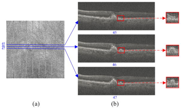
Widely used clinical OCT scan patterns densely sample the field-of-view, so as to not miss small abnormalities, and thus result in highly correlated neighboring B-scans. (a) Summed-voxel projection [38] en face SDOCT image of a non-neovascular age-related macular degeneration (AMD) patient from the Age-Related Eye Disease Study 2 (AREDS2) Ancillary SDOCT (A2A SDOCT) [39]. (b) Three B-scans acquired from adjacent positions. The red rectangular regions are zoomed in to better demonstrate the differences between these neighboring scans.

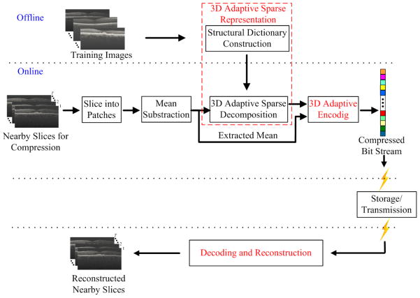
Therefore, we propose the 3D-ASRC algorithm for the compression of 3D OCT images, which can utilize the high correlations while still considering the differences of nearby slices. The proposed 3D-ASRC method is composed of three main parts: a) 3D adaptive sparse representation; b) 3D adaptive encoding; c) decoding and reconstruction, which will be described in the following subsections. The outline of the proposed 3D-ASRC algorithm is illustrated in Fig. 2.

Fig.2.

Outline of the proposed 3D-ASRC algorithm.

A. 3D Adaptive Sparse Representation

We divide a volume of OCT B-scans into several groups, each with T nearby slices according to the similarities among them [40]. Similar to the 2D sparse compression schemes [29–32], each slice in an OCT volume is partitioned into many non-overlapping patches and the mean of each patch is subtracted from them. We define nearby patches as a set of patches centered around the patch ${\mathbf{x}}_i^1$ from slices in the same group as ${\left\{{\mathbf{x}}_i^t\right\}}_{t=1}^T$, where t denotes a particular B-scan in that group. Similar to the 2D case, the parameter i in ${\left\{{\mathbf{x}}_i^t\right\}}_{t=1}^T$ indexes patches that are centered at the same lateral and axial positions in each of the T azimuthally distanced 2D nearby slices. By rewriting equation (2), the sparse coefficient vectors ${\left\{{\mathbf{\alpha }}_i^t\right\}}_{t=1}^T$ of the nearby patches ${\left\{{\mathbf{x}}_i^t\right\}}_{t=1}^T$ can be obtained from optimizing:

$${\left\{{\widehat{\mathbf{\alpha }}}_i^t\right\}}_{t=1}^T=arg\underset{{\mathbf{\alpha }}_i^t}{min}\sum _{t=1}^T{\Vert {\mathbf{\alpha }}_i^t\Vert }_0\text{subject}\text{to}\sum _{t\in \{1,\dots ,T\}}{\Vert {\mathbf{x}}_i^t-\mathbf{D}{\mathbf{\alpha }}_i^t\Vert }_2^2\le \epsilon$$ (7)

To solve (7), we propose an offline structural dictionary learning strategy from a training dataset and an online 3D adaptive sparse decomposition algorithm for obtaining the sparse coefficients vectors. As described in [41], solving (7) has the denoising effect, which is based on the sparsity based denoising scheme. Specifically, such a sparsity scheme assumes that the dictionary D is pre-learned from a set of images (or patches) with negligible noise content. Then, while the true signal (e.g. containing only anatomically relevant information) can be accurately represented by a very low number of combinations of the atoms selected from the dictionary, the noise cannot be represented with a limited number of dictionary atoms. Then, if the sparse coefficients ${\widehat{\mathbf{\alpha }}}_i^t$ (corresponding to the selected dictionary atoms) for an input noisy patch ${\mathbf{x}}_i^t$ are obtained, we can reconstruct the corresponding noiseless patch estimate ${\widehat{\mathbf{x}}}_i^t$ by multiplying dictionary D with the sparse coefficients ${\widehat{\mathbf{\alpha }}}_i^t$.

1) Structural Dictionary Construction

We learn the appropriate overcomplete dictionary of basis functions from a set of high-quality training data. Since raw OCT images are often very noisy [42], to attain high signal-to-noise (SNR) images, we capture, register, and average repeated low-SNR B-scans from spatially very close positions [23]. Note that unlike test data, which is captured in clinical settings, training data is only captured once from volunteers and can utilize lengthier (albeit limited by the ANSI standard for maximum permissible exposure to a light beam) scan patterns than the faster clinical scan protocols. Also, dictionary construction is an offline (one-time) process and does not add to the computational cost of compressing clinical images.

The conventional K-SVD algorithm [35] learns one universal dictionary from a large number of training patches. Typical clinical OCT images may contain many complex structures (e.g. retinal OCT scans show different layers and pathologies such as cysts [43]) and thus one universal dictionary D might not be optimal for representing these varied structures. Therefore, following our previous works in [20, 21], we learn H sets of structural sub-dictionaries $\left\{{\mathbf{D}}_h^{\text{structural}}\in {ℝ}^{q\times n}\right\}$, h = 1,…,H, each designed to represent one specific type of structure. This is achieved by first adopting the k-means approach to divide the training patches into H clusters. For each cluster h, one sub-dictionary ${\mathbf{D}}_h^{\text{structural}}$ is learned by the K-SVD algorithm [35] and one centroid c_h ∈ ℝ^q patch is also obtained by the k-means approach.

2) 3D Adaptive Sparse Decomposition

Our sparse compression algorithm is designed to exploit similarities in neighboring slices of clinical OCT scans, as illustrated in Fig. 1(b). To achieve this, in the first step we search for the structural sub-dictionary that is most suitable to represent each test patch ( ${\mathbf{x}}_i^t$). We use the Euclidian distance between the patch and the sub-dictionary centroid c_h for selecting the appropriate sub-dictionary ${\mathbf{D}}_{{\widehat{h}}_i^t}^{\text{structural}}$:

$${\widehat{h}}_i^t=arg\underset{h_i^t}{min}{\Vert {\mathbf{c}}_h-{\mathbf{x}}_i^t\Vert }_2^2,t=1,\dots ,T,\text{and}h=1,\dots ,H.$$ (8)

In the second step, we find the set of sparse coefficients corresponding to such sub-dictionaries to best represent a set of nearby patches ${\left\{{\mathbf{x}}_i^t\right\}}_{t=1}^T$. Indeed, it would have been optimal if we could utilize a single sub-dictionary for each set of nearby patches. However, such an approach results in low-quality reconstruction of poorly correlated nearby patches in the receiver side. This is because the nearby slices might still have large localized differences (see the areas labeled with the red rectangles in Fig. 1(b)) and so one sub-dictionary designed for one kind of structure cannot effectively account for these differences. To address this issue, we utilize index ${\left\{{\widehat{h}}_i^t\right\}}_{t=1}^T$ to define two classes of nearby patches: “similar” and “different”. In a similar set of patches ( ${\left\{{\mathbf{x}}_{\text{sim},i}^t\right\}}_{t=1}^T$), all patches correspond to the same sub-dictionary, while in a different set of patches ${\left\{{\mathbf{x}}_{\text{dif},i}^t\right\}}_{t=1}^T$, each patch may correspond to different sub-dictionaries.

The “similar” nearby patches are highly compressible as they can be jointly represented by the same atoms from the commonly selected sub-dictionary ${\mathbf{D}}_{{\widehat{h}}_i^{\mathit{com}}}^{\text{structural}}$. This is achieved by invoking the row-sparsity condition [44] in the sparse coefficients matrix ${\mathbf{A}}_{\text{sim},i}=\left[{\mathbf{\alpha }}_{\text{sim},i}^1,\dots ,{\mathbf{\alpha }}_{\text{sim},i}^T\right]$:

$${\widehat{\mathbf{A}}}_{\text{sim},i}=arg\underset{{\widehat{\mathbf{A}}}_{\text{sim},i}}{min}{\Vert {\mathbf{A}}_{\text{sim},i}\Vert }_{\text{row},0}\text{subject}\text{to}\sum _{t\in \{1,\dots ,T\}}{\Vert {\mathbf{x}}_{\text{sim},i}^t-{\mathbf{D}}_{{\widehat{h}}_i^{\mathit{com}}}^{\text{structural}}{\mathbf{\alpha }}_{\text{sim},i}^t\Vert }_2^2\le \epsilon ,$$ (9)

where ||•||_row,0 stands for the joint sparse norm [44, 45], which is used to select a small number of most representative non-zero rows in A_sim,i. We utilize a variant of the OMP algorithm called simultaneous OMP (SOMP) [44] to solve this problem. In Â_sim,i, while the values of the nonzero coefficients in different sparse vectors ${\mathbf{\alpha }}_{\text{sim},i}^1,\dots ,{\mathbf{\alpha }}_{\text{sim},i}^T$ might be different, their positions are the same, a property which we will exploit in the next subsection for enhanced compression.

A simple trick that can help us further reduce the total number of nonzero coefficients needed to represent a similar set of patches is to estimate the variance of the sparse vectors ${\left\{{\widehat{\mathbf{\alpha }}}_{\text{sim},i}^t\right\}}_{t=1}^T$. If the variance of the sparse vectors in a set is below a threshold, we denote this set as “very similar” and then fuse the corresponding sparse vectors into one vector α_vs,i.. Otherwise, we denote them as “not very similar” ${\left\{{\mathbf{\alpha }}_{\text{nvs},i}^t\right\}}_{t=1}^T$ and keep all the coefficients:

$$\{\begin{array}{l}{\mathbf{\alpha }}_{v\mathrm{s},i}=\text{mean}{\left\{{\mathbf{\alpha }}_{\text{sim},i}^t\right\}}_{t=1}^T,\text{if}\text{variance}\left({\left\{{\mathbf{\alpha }}_{\text{sim},i}^t\right\}}_{t=1}^T\right)\le b•\epsilon \hfill \\ {\left\{{\mathbf{\alpha }}_{\text{nvs},i}^t\right\}}_{t=1}^T={\left\{{\mathbf{\alpha }}_{\text{sim},i}^t\right\}}_{t=1}^T,\text{if}\text{variance}\left({\left\{{\mathbf{\alpha }}_{\text{sim},i}^t\right\}}_{t=1}^T\right)>b•\epsilon \hfill \end{array},$$ (10)

where b is a constant and the mean is the operation to compute the mean of the ${\left\{{\mathbf{\alpha }}_{\text{vs},i}^t\right\}}_{t=1}^T$.

The “different” nearby patches ${\left\{{\mathbf{x}}_{\text{dif},i}^t\right\}}_{t=1}^T$ are independently decomposed on the sub-dictionaries ${\mathbf{D}}_{{\widehat{h}}_i^t}^{\text{structral}}$ that can best fit each of them, which amounts to the problem:

$${\left\{{\widehat{\mathbf{\alpha }}}_{\text{dif},i}^t\right\}}_{t=1}^T=arg\underset{{\mathbf{\alpha }}_{\text{dif}}^t}{min}\sum _{t=1}^T{\Vert {\mathbf{\alpha }}_{\text{dif},i}^t\Vert }_0\text{subject}\text{to}\sum _{t\in \{1,\dots ,T\}}{\Vert {\mathbf{x}}_{\text{dif},i}^t-{\mathbf{D}}_{{\widehat{h}}_i^t}^{\text{structural}}{\mathbf{\alpha }}_{\text{dif},i}^t\Vert }_2^2\le \epsilon .$$ (11)

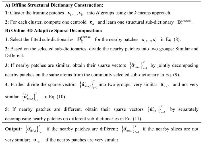
We solve this problem by applying the OMP algorithm [37] separately on each patch. Note that the positions and values of the nonzero coefficients in ${\left\{{\widehat{\mathbf{\alpha }}}_{\text{dif},i}^t\right\}}_{t=1}^T$ might be varied for reflecting the differences among the nearby patches ${\left\{{\mathbf{x}}_{\text{dif},i}^t\right\}}_{t=1}^T$. The proposed 3D sparse representation algorithm is summarized in Fig. 3.

Fig. 3.

3D adaptive sparse representation algorithm.

B. 3D Adaptive Encoding

To encode the positions and values of the nonzero coefficients representing a set of nearby patches, we first quantize the sparse vectors using a uniform quantizer [31]. Then, we utilize an adaptive strategy to preserve the positions and values of the nonzero coefficients as follows:

1. For the “very similar” nearby patches, both the positions and values of the nonzero coefficients are the same and these sparse vectors are already fused into one vector α_vs,i. Thus, only one sequence is required to store the position information and one sequence is used to preserve the value information, as shown in Fig. 4(a).

2. For the “not very similar” nearby patches, the positions of the nonzero coefficients in ${\left\{{\mathbf{\alpha }}_{\text{nvs},i}^t\right\}}_{t=1}^T$ are the same while their values are different. Thus, only one sequence is needed to store the position information while another T sequences are employed to preserve the value information, as shown in Fig. 4 (b).

3. For the “different” nearby patches the positions and values of the nonzero coefficients in ${\left\{{\widehat{\mathbf{\alpha }}}_{\text{dif},i}^t\right\}}_{t=1}^T$ are different. Thus, the position information is preserved using T different sequences, while the value information is stored with other T different sequences, as shown in Fig. 4 (c).

Fig. 4.

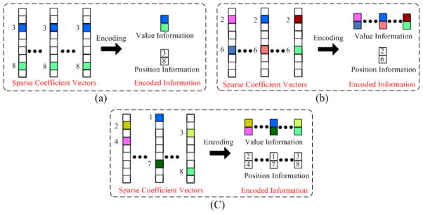
3D adaptive encoding for the three classes of the nearby sparse vectors (a) Very similar; (b) Not very similar; (c) Different. Note that the color blocks in the sparse vectors denote the nonzero coefficients. Different colors represent different values.

We label the three classes (“Very similar”, “Not very similar”, and “Different”) of nearby slices as 0, 1, and 2, respectively. These class types are stored in one sequence. In addition, the means ${\left\{m_i^t\right\}}_{t=1}^T$ of nearby patches ${\left\{{\mathbf{x}}_i^t\right\}}_{t=1}^T$ are quantized and put into T different sequences. Furthermore, indexes ${\left\{h_i^t\right\}}_{t=1}^T$ of the selected sub-dictionaries for nearby patches are stored with another T sequences. Finally, we apply Huffman coding [46] on the above sequences to create a one bit stream.

C. Decoding and Image Reconstruction

At the decoding site, given the compressed bit stream, we first extract the mean ${\left\{m_i^t\right\}}_{t=1}^T$, sparse vectors ${\left\{{\mathbf{\alpha }}_i^t\right\}}_{t=1}^T$, and indexes ${\left\{h_i^t\right\}}_{t=1}^T$ of the selected sub-dictionaries for each set of nearby patches. Then, a set of nearby patches ${\left\{{\mathbf{x}}_i^t\right\}}_{t=1}^T$ are reconstructed by a simple linear operation,

$${\mathbf{x}}_i^t={\mathbf{D}}_{h_i^t}^{\text{structural}}{\mathbf{\alpha }}_i^t+m_i^t,t=1,\dots ,T.$$ (12)

Subsequently, each patch ${\widehat{\mathbf{x}}}_i^{t_s}$ (where t_s denotes a specific patch) is further enhanced by weighted averaging of the nearby patches: ${\widehat{\mathbf{x}}}_i^{t_s}={\displaystyle \sum _{t=1}^T}{w}_i^{t,t_s}{\widehat{\mathbf{x}}}_i^t$, where $w_i^{t,t_s}$ [20] is estimated as:

$$w_i^{t,t_s}=\frac{exp\left(-{\Vert {\widehat{\mathbf{x}}}_i^t-{\widehat{\mathbf{x}}}_i^{t_s}\Vert }_2^2/h\right)}{\text{Norm}}.$$ (13)

In (13), Norm is defined as ${\displaystyle \sum _{t=1}^T}exp\left(-{\Vert {\widehat{\mathbf{x}}}_i^t-{\widehat{\mathbf{x}}}_i^{t_s}\Vert }_2^2/h\right)$ and h is a predefined scalar. Finally, we recover each B-scan by combining its reconstructed patches in a raster-scan order.

IV. Experimental Results

To validate the effectiveness of the proposed 3D-ASRC algorithm, we compared its performance with those of four well-known compression approaches: JPEG 2000, MPEG-4, SPIHT [47], K-SVD [29], and three variants of the proposed algorithm: SRC-Dif, 2D-ASRC, 3D-ASRC-WA. We emulated the JPEG 2000 method with “imwrite” function in the Matlab 2012a [48] and the MPEG-4 method with the “export” function in QuickTime Player Pro 7.0 software [49]. We implemented the SPIHT method with the Matlab code downloaded from [50]. For the K-SVD method, we first learn only one dictionary from a large number of training patches off-line and then use this dictionary for the compression as detailed in [29]. For the SRC-Dif method, we utilize the “different-patch” based sparse representation and encoding scheme for compression. Note that, in final reconstruction stage, the 3D weighted averaging technique utilized in the proposed 3D-ASRC method is also applied to the SRC-Dif method. For the 2D-ASRC method, instead of using the temporal nearby patches among the nearby slices, we denoted a number of spatial nearby patches within one slice as the nearby patches. Then, we utilized the adaptive sparse representation algorithm for the compression of the spatial nearby patches. For the 3D-ASRC-WA method, we do not use the 3D weighted averaging technique for the final reconstruction, compared to the 3D-ASRC method.

A. Data Sets

In our experiments, we first used volumetric scans of human retinas from 26 different subjects with and without non-neovascular AMD, imaged by an 840-nm wavelength SDOCT system from Bioptigen, Inc. (Durham, NC, USA) with an axial resolution of ~4.5 μm per pixel in tissue. This dataset is part of the A2A SDOCT clinical trial [39], which was already utilized in our previous works for denoising and interpolation of SDOCT images [20, 23], and is freely available online¹. Each patient was imaged twice. The first scan was a 6.6×6.6 mm² volume with 100 B-scans and 1000 A-scans including the fovea. The second scan was centered at the fovea with 40 azimuthally repeated B-scans each with 1000 A-scans spanning 6.6 mm. Since these SDOCT images were very noisy, we first registered the second set of B-scans with the StackReg image registration plug-in [51] in ImageJ and then averaged them to create a less noisy image of the fovea. The averaged image for each dataset was then used as the reference image to compute quantitative metrics of image quality. From these 26 datasets, we randomly selected 16 subjects to test the performance of the proposed method while the remaining datasets from the other 10 subjects were used to train the dictionary and set algorithmic parameters. The subjects and the related datasets used in the dictionary training phase were strictly separated from those used in the testing phase. Following the work in [20], we chose to train our images based on the B-scans from the foveal area, since they contain more diverse structures as compared to more peripheral scans. In the 16 human datasets, the average percentage of patches labeled as “similar” in the proposed 3D-ASRC method is 83.4%.

In addition, we also performed our experiments on a mouse dataset acquired by a different SDOCT system, (Bioptigen Envisu R2200), with ~ 2μm axial resolution in tissue. The acquired volume was centered at the optic nerve with 100 B-scans and 1000 A-scans. For compressing the mouse dataset, we used the same algorithmic parameters and dictionaries learned from the human retina, to demonstrate the robustness of this algorithm for compressing images from different imaging scenarios. In the mouse dataset, the percentage of the patches labeled as “similar” in the proposed 3D-ASRC method is 81.2%.

For both mouse and human data, each A-scan included 1024 pixels. In most retinal SDOCT images, the relevant anatomical information is only present in a fraction of the imaged space. Thus, we cropped all A-scans to 360 pixels for human data and to 370 pixels for mouse data, which corresponded to the most relevant anatomic data. All images shown in Figs. 5–8 are of size 360×1000 while images in Fig. 9, 10 are of size 370×1000. All quantitative comparisons for both the human and mouse data are based on slightly larger cropped images of size 450× 1000, to exclude the smooth dark areas below the choroid or in the vitreous.

Fig. 5.

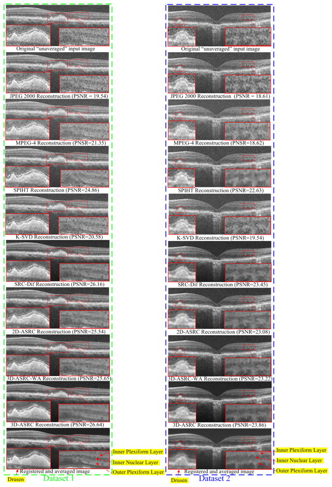
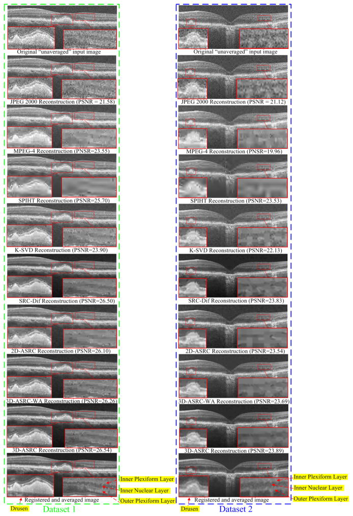
Reconstructed results using JPEG 2000, MPEG-4, SPIHT [47], K-SVD [29], SRC-Dif, 2D-ASRC, 3D-ASRC-WA and 3D-ASRC methods with compression ratio=10 on two human retinal datasets.

Fig. 8.

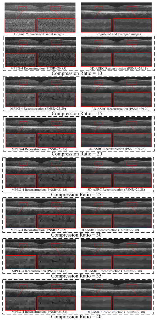
Comparison of reconstructed results using MPEG-4 and the proposed 3D-ASRC methods under seven different compression ratios (ranging from 10 to 40) on a human retinal image.

Fig. 9.

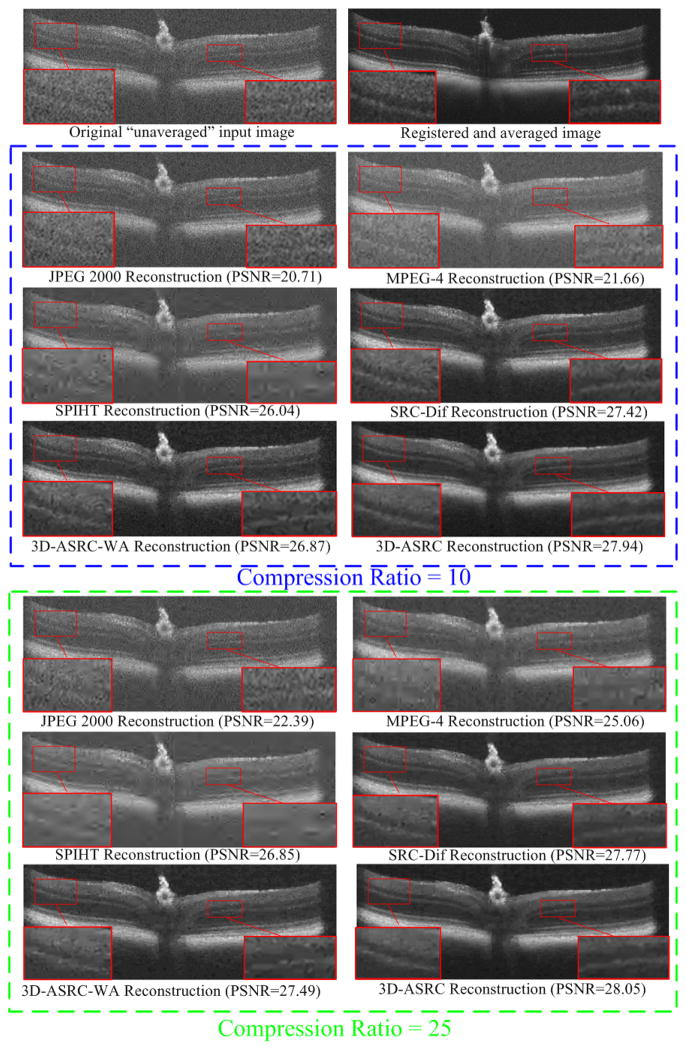
Reconstructed results using JPEG 2000, MPEG-4, SPIHT [47], SRC-Dif, 3D-ASRC-WA and the 3D-ASRC methods with compression ratios of 10 and 25 on one mouse retinal dataset.

Fig. 10.

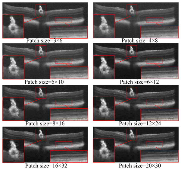
Effects of different patch sizes (from 3×6 to 20×30) on the performance of the proposed 3D-ASRC method on the mouse data.

B. Algorithm Parameters

Based on our experiments on training data, we empirically selected the parameters for the proposed 3D-ASRC algorithm. Since most of the meaningful structures (e.g., different layers) in retinal OCT images are horizontally oriented, we chose the patch size in each slice to be a rectangle of size 6×12 pixels (height×width). The number of nearby slices T was set to 5 (corresponding to ~300 microns azimuthal distance). In retinal imaging, slices from farther distances may have significant differences and thus adding them might actually reduce compression efficiency. In the dictionary training stage, the value of cluster H was chosen to be 10. In each cluster, the size of the trained dictionary was set to 72×500. Using a larger cluster number and dictionary size might enhance the effectiveness of the compression, but also result in the higher computational cost. The parameter b in (10) was set to 0.001. The above parameters were kept unchanged for all the test images to demonstrate the robustness of the algorithm to these empirically selected parameters. To control the compression ratio in different experiments, we tuned the parameter C in the error tolerance ε of (9) and (11) (e.g. the larger the value of C, the higher the compression ratio). Naturally, as the information content of different images varies, to achieve the exact same compression ratio the parameter C should be slightly changed for different datasets. For the test datasets in our experiments, the mean and standard deviation of parameter C for the compression ratios=[10, 15, 20, 25, 30, 35, 40] were [1.00, 1.07, 1.12, 1.15, 1.17, 1.19, 1.21], and [0.053, 0.054, 0.052, 0.055, 0.055, 0.057, 0.059 ], respectively. The parameters for the JPEG 2000 and MPEG-4 were set to the default values in the Matlab [48] and QuickTime Player Pro 7.0 software [49], respectively. For the K-SVD algorithm, the patch size was set to 6×12 and the trained dictionary was of size 72×500, which were similar to what was used for our 3D-ASRC method. For the 2D-ASRC method, the number of spatial nearby patches was selected to 9 and the other parameters were set to the same values as in our 3D-ASRC method.

C. Quantitative Metrics

We adopted the peak signal-to-noise-ratio (PSNR) and feature similarity index measure (FSIM) [52] to evaluate the performances of the compression methods. The PSNR and FSIM calculations require a high-quality reference image. Since our experiments are based on real data (not simulation), we used the registered and averaged images obtained from the azimuthally repeated scans as the reference image. We registered the reference image and reconstructed images using the StackReg technique [51] to significantly reduce the motion between them.

D. Experiments on Human Retinal SDOCT Images

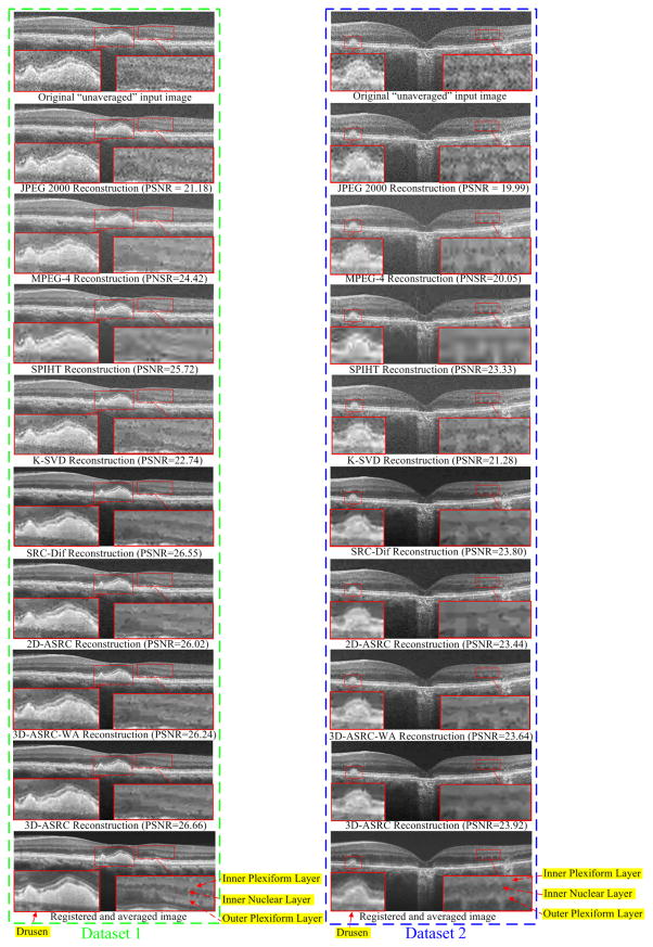
We tested the JPEG 2000, MPEG-4, SPIHT [47], K-SVD [29], SRC-Dif, 2D-ASRC, 3D-ASRC-WA, and 3D-ASRC methods on seven different compression ratios ranging from 10 to 40. Figs. 5–7 show qualitative comparisons of reconstructed results from the tested methods using the compression ratios of 10, 25, and 40, respectively. Since boundaries between retinal layers and drusen contain meaningful anatomic and pathologic information [53], we magnified one boundary area and one dursen area in each figure. As can be observed in Fig. 5, results from JPEG 2000, K-SVD, and MPEG-4 methods appear very noisy with indistinct boundaries for many important structural details (see the zoomed boundary areas of both the dataset 1 and 2). The SPIHT method greatly suppresses noise, but increases blur and introduces visible artifacts (see the zoomed drusen and boundary areas of both the dataset 1 and 2). Compared to the above methods, the proposed 2D-SDL, SRC-Dif, 2D-ASRC, 3D-ASRC-WA methods deliver comparatively better structural details, but still shows some noise artifacts. By contrast, the proposed 3D-ASRC method achieves noticeably improved noise suppression, and preserves meaningful anatomical structures, even at very high compression rates, as illustrated in Fig. 6 and Fig. 7.

Fig. 7.

Reconstructed results using JPEG 2000, MPEG-4, SPIHT [47], K-SVD [29], SRC-Dif, 2D-ASRC, 3D-ASRC-WA and 3D-ASRC methods with compression ratio=40 on two human retinal datasets.

Fig. 6.

Reconstructed results using JPEG 2000, MPEG-4, SPIHT [47], K-SVD [29], SRC-Dif, 2D-ASRC, 3D-ASRC-WA and 3D-ASRC methods with compression ratio=25 on two human retinal datasets.

The proposed 3D-ASRC method has improved performance over the SRC-Dif method mainly because the joint sparse solution (for equation (9)) utilized in the proposed 3D-ASRC method can exploit correlations among nearby patches that are similar, and is more robust to noise interferences. Specifically, the key for the sparse solution is the selection of optimal dictionary atoms for the representation of input patches, which can be negatively affected by heavy noise. The SRC-Dif method is more prone to noise artifacts because each patch separately selects its suitable atom without consideration of possible correlations among nearby patches. In contrast, the proposed 3D-ASRC method exploits correlations among nearby patches, as the nearby patches can jointly select their common atoms. Jointly exploiting correlations among similar patches to select the atoms is similar to the idea of the majority voting method [54]. That is, if the decisions of several patches are jointly considered, the final decision is usually more robust to external disturbances and thus the jointly selected atom is expected to be better than each of the separately selected atoms. Therefore, the reconstructed visual results of the proposed 3D-ASRC method present less noise and artifacts than those of the SRC-Dif method. This observation is in line with other recent works [23, 55, 56] that have also demonstrated that exploiting correlations among similar patches can achieve better representation and thus leads to improved performance in other image restoration applications. In addition, in cases of high compression ratios (e.g. 40), some meaningful structures in the visual results of the SRC-Dif method are more blurred than those of the 3D-ASRC method (see the zoomed drusen and layer boundary areas of Dataset 2 in Fig. 7). The improved image quality for such high compression ratio conditions is mainly due to efficient reduction of storage for sparse coefficients in the proposed 3D adaptive representation and encoding scheme. Thus, compared with the SRC-Dif method, under the same compression ratio, the proposed 3D-ASRC method can use more sparse coefficients (corresponding to meaningful dictionary atoms) to better reconstruct the structures in the original OCT image.

Fig. 8 illustrates visual comparisons of reconstructed images of the MPEG-4 and the proposed 3D-ASRC methods under seven different compression ratios. As can be observed, the proposed 3D-ASRC method can generally preserve retinal layer structures and boundaries for different compression ratios. In contrast, under low compression ratios (e.g. 10 and 15), the results using the MPEG-4 method appear very noisy, while some meaningful structures are over-smoothed for higher compression ratios (e.g. from 25 to 40).

Quantitative comparisons (PSNR and FSIM) of all the test methods at different compression ratios are reported in Tables I. Note that we can only compute the PSNR and FSIM for the one noiseless image (from the fovea) in each dataset. As can be seen in Table I, the proposed 3D-ASRC method consistently delivered better PSNR and FSIM results than the other methods. At higher compression rates, the PSNR and FSIM results of all the methods generally first improved and then became stable, or even decreased. This is because input images are noisy and the inherent smoothing of the compression methods reduces the noise level and thus improves PSNR.

Table I.

Mean of the PSNR and FSIM for 16 Foveal Images from 16 Different Subjects Reconstructed by JPEG 2000, MPEG-4, SPIHT [47], K-SVD [29], SRC-Dif, 2D-ASRC, 3D-ASRC-WA, and 3D-ASRC Under Seven Different Compression Ratios Ranging from 10–40.

Method/Compression ratio	10	15	20	25	30	35	40
JPEG 2000	19.67/0.65	20.33/0.67	20.70/0.69	21.34/0.70	21.92/0.70	22.41/0.71	22.78/0.71
MPEG-4	20.42/0.72	22.44/0.78	22.63/0.79	22.71/0.79	22.76/0.79	23.21/0.78	23.22/0.79
SPIHT	25.56/0.80	26.17/0.82	26.50/0.82	26.68/0.82	26.79/0.82	26.86/0.82	26.89/0.82
K-SVD	20.74/0.68	22.51/0.70	22.51/0.72	23.06/0.74	23.56/0.75	23.94/0.75	24.28/0.76
SRC-Dif	26.98/0.85	27.26/0.86	27.45/0.87	27.54/0.87	27.56/0.87	27.58/0.86	27.55/0.86
2D-ASRC	26.14/0.81	26.51/0.82	26.73/0.82	26.85/0.83	26.89/0.83	26.91/0.83	26.99/0.83
3D-ASRC-WA	26.31/0.82	26.70/0.83	26.97/0.84	27.11/0.85	27.23/0.85	27.29/0.85	27.33/0.85
3D-ASRC	27.60/0.88	27.65/0.87	27.68/0.87	27.71/0.87	27.75/0.87	27.75/0.87	27.74/0.87

Also, we report the average (over 16 human retinal datasets) running time of the proposed 3D-ASRC algorithm and the compared approaches for the compression and reconstruction of one human retinal image on Table II. All the programs are executed on a laptop computer with an Intel (R) Core i7-3720 CPU 2.60 GHz and 8 GB of RAM. Note that the sparsity based methods SRC-Dif, 3D-ASRC-WA, 2D-ASRC, and 3D-ASRC algorithms were coded in MATLAB, which is not optimized for speed. If more efficient coding coupled with a general purpose graphics processing unit (GPU) were adopted, the running time of these sparsity based methods are expected to be reduced significantly.

Table II.

The Average Running Time (seconds) for the Compression and Reconstruction of One Human Retinal Image by the JPEG 2000, MPEG-4, SPIHT [47], K-SVD [29], SRC-DIF, 2D-ASRC, 3D-ASRC-WA, AND 3D-ASRC METHODS Under SEVEN Different Compression Ratios Ranging from 10–40. In this Table, “Com” Denotes the Required Time for the Compression Stage while the “Rec” Stands for the Required Time for the Reconstruction Stage.

Method/Compression Ratio	10		15		20		25		30		35		40
	Com	Rec	Com	Rec	Com	Rec	Com	Rec	Com	Rec	Com	Rec	Com	Rec
JPEG 2000	0.04	0.01	0.04	0.01	0.04	0.01	0.04	0.01	0.04	0.01	0.04	0.01	0.04	0.01
MPEG-4	0.66	0.02	0.64	0.02	0.62	0.02	0.58	0.02	0.53	0.02	0.47	0.02	0.45	0.02
SPIHT	2.41	1.23	1.28	0.63	0.91	0.46	0.83	0.35	0.68	0.27	0.59	0.28	0.58	0.24
SRC-Dif	3.43	2.68	2.63	2.27	2.17	1.85	1.88	1.83	1.69	1.73	1.41	1.56	1.36	1.23
2D-ASRC	2.82	2.01	2.11	1.65	1.73	1.24	1.53	1.21	1.41	1.13	1.24	0.96	1.23	0.64
3D-ASRC-WA	2.93	2.04	2.18	1.66	1.78	1.26	1.57	1.22	1.43	1.14	1.26	0.97	1.24	0.64
3D-ASRC	2.93	2.61	2.18	2.23	1.78	1.83	1.57	1.79	1.43	1.71	1.26	1.54	1.24	1.21

E. Experiments on Mouse Retinal SDOCT Images

Fig. 9 shows qualitative and quantitative comparisons of results from the mouse dataset reconstructed by JPEG 2000, MPEG-4, SPIHT [47], SRC-Dif, 3D-ASRC-WA and 3D-ASRC methods using the compression ratios of 10 and 25, respectively. In this experiment, we used the same sparse dictionary as in our human experiments. Note that the SDOCT imaging system for acquiring the mouse images had a different axial resolution and used a different spectrometer compared to the one used for the acquisition of human images. Therefore, using the dictionary learned from human data would be sub-optimal to represent mouse data. Despite this fact, the proposed 3D-ASRC method generally delivered better results than the compared methods. The main reason why the dictionary trained on human datasets can be used to accurately represent mouse data is due to the small patch size. Specifically, instead of representing large structures (e.g. optical nerve head in the mouse data) on the test image as a whole, the sparse representation seeks the best-matched atoms from a large dictionary to represent small regions of the large structures. Although the large structures from the mouse data do not exist in the human dictionary, each small region in the large structures can be accurately represented by a set of similar atoms in the human dictionary and thus these small regions can be combined to accurately reflect the large structures.

To test the effect of different patch sizes on performance of the 3D-ASRC method on mouse data, we vary the patch sizes from 3×6 to 20×30. The qualitative results of the 3D-ASRC method using different patch sizes with compression ratio=25 are illustrated in Fig. 10. As can be observed, when the patch sizes are very small (e.g. 3×6 and 4×8), the optical nerve head area exhibits obvious block artifacts. This is due to the fact that under comparatively high compression ratios, patch sizes that are too small will lead to an insufficient number of sparse coefficients (corresponding to dictionary atoms) for representing these small patches. As the patch size increases, the block artifacts start to disappear and the reconstructed results will appear smoother. However, when the patch sizes are very large (e.g. from 12×24 to 20×30), some meaningful structures (e.g. drusen and layers in the zoomed areas) become blurred. This is because structures within the large patches of the mouse image might not find the corresponding matched atoms in the human dictionary and thus may not be well represented.

V. Conclusions

In this paper, we presented a novel sparsity based method named 3D-ASRC for efficient compression of 3D SDOCT images. Unlike the previous sparsity based methods designed for 2D images, the 3D-ASRC method simultaneously represents the nearby slices of the SDOCT images via a 3D adaptive sparse representation algorithm. Such a 3D adaptive algorithm exploits similarities among nearby slices, yet is sensitive in preserving their differences. Our experiments on the 2D version of the proposed algorithm (2D-ASRC) showed that even in the absence of information from neighboring scans, the proposed algorithm is a powerful tool for compression of OCT images. Our experiments on real clinical grade SDOCT datasets demonstrated the superiority of the proposed 3D-ASRC method over several well-known compression methods, in terms of both visual quality and quantitative metrics. Experiments on the mouse dataset attested to the robustness of the algorithm to the differences between the dataset from which the dictionary is learned and the data that is to be compressed. Indeed, any compression algorithms, including our proposed method, introduce unique compression artifacts. The imaging artifacts of the competing techniques are described in the literature (e.g. wavelet artifacts are clearly visible in Fig.7 for the SPIHT method) [57]. The dominant imaging artifact of our proposed method is the piecewise constant artifact, which may result in the loss of some features such as small inner retinal vessels. However, for some clinical applications, including retinal layer segmentation, the piecewise constant artifact is less problematic, as it even further accentuates the boundaries between retinal layers.

In this paper, the correlations among the “similar” patches of the nearby slices are utilized. We expect that by utilizing a larger number of “similar” patches we can further improve the compression rate of the proposed technique. Therefore, one of our future works is to adopt the nonlocal searching technique [55, 58] to find more “similar” patches in both inter and intra slice.

In this paper, we demonstrated the applicability of our algorithm for compression of ophthalmology OCT datasets. The algorithm described here is directly applicable to other imaging scenarios, although its relative effectiveness compared to other techniques when applied to images with different noise and signal statistics is yet to be determined. In our future publications, we will investigate the applicability of our method for analyzing a wide variety of OCT images from different tissues (e.g. dermatology [59], Gastroenterology [60], and cardiology [61]). In addition, there is a strong incentive to apply the proposed 3D adaptive sparse representation algorithm to other large-scale inverse imaging applications (e.g., 3D image reconstruction [62], denoising, deblurring, and super-resolution) and also for compressing other types of medical images including those from MRI, tomosynthesis, and X-ray computed tomography.

Table III.

Mean of PSNR and FSIM for 16 Foveal Images from 16 Different Subjects Reconstructed by the JPEG 2000, MPEG-4, SPIHT , SRC-Dif, 3D-ASRC-WA, and 3D-ASRC Methods Under Seven Different Compression Ratios Ranging from 10–40.

Method/Compression ratio	10	15	20	25	30	35	40
JPEG 2000	20.71/0.70	21.63/0.73	22.10/0.74	22.39/0.76	22.62/0.77	22.89/0.78	23.26/0.78
MPEG-4	21.66/0.77	22.85/0.79	24.99/0.82	25.06/0.83	25.11/0.83	25.11/0.93	25.11/0.83
SPIHT	26.04/0.82	26.51/0.83	26.72/0.83	26.85/0.83	26.97/0.82	27.04/0.82	27.10/0.82
SRC-Dif	27.42/0.85	27.51/0.85	27.69/0.85	27.77/0.84	27.84/0.84	27.89/0.84	27.89/0.83
3D-ASRC-WA	26.87/0.83	27.18/0.84	27.37/0.84	27.49/0.84	27.55/0.84	27.58/0.83	27.63/0.83
3D-ASRC	27.94/0.86	27.96/0.86	27.99/0.85	28.05/0.85	28.06/0.84	28.07/0.84	28.08/0.84

References

- 1.Bhat S, Larina IV, Larin KV, Dickinson ME, Liebling M. 4D reconstruction of the beating embryonic heart from two orthogonal sets of parallel optical coherence tomography slice-sequences. IEEE Trans Med Imag. 2013 Mar;32(3):578–588. doi: 10.1109/TMI.2012.2231692. [DOI] [PMC free article] [PubMed] [Google Scholar]
- 2.Huang D, Swanson EA, Lin CP, Schuman JS, Stinson WG, Chang W, Hee MR, Flotte T, Gregory K, Puliafito CA, Fujimoto JG. Optical coherence tomography. Science. 1991 Nov;254(5035):1178–1181. doi: 10.1126/science.1957169. [DOI] [PMC free article] [PubMed] [Google Scholar]
- 3.Ehlers JP, Tao K, Farsiu S, Maldonado R, Izatt JA, Toth CA. Integration of a spectral domain optical coherence tomography system into a surgical microscope for intraoperative imaging. Invest Ophthalmol Vis Sci. 2011 May;52(6):3153–3159. doi: 10.1167/iovs.10-6720. [DOI] [PMC free article] [PubMed] [Google Scholar]
- 4.Nankivil D, Dhalla AH, Gahm N, Shia K, Farsiu S, Izatt JA. Coherence revival multiplexed, buffered swept source optical coherence tomography: 400RRkHz imaging with a 100RRkHz source. Opt Lett. 2014 Jul;39(13):3740–3743. doi: 10.1364/OL.39.003740. [DOI] [PMC free article] [PubMed] [Google Scholar]
- 5.Klein T, Wieser W, Reznicek L, Neubauer A, Kampik A, Huber R. Multi-MHz retinal OCT. Biomed Opt Exp. 2013 Aug;4(10):1890–1908. doi: 10.1364/BOE.4.001890. [DOI] [PMC free article] [PubMed] [Google Scholar]
- 6.Wieser W, Draxinger W, Klein T, Karpf S, Pfeiffer T, Huber R. High definition live 3D-OCT in vivo: design and evaluation of a 4D OCT engine with 1 GVoxel/s. Biomed Opt Express. 2014 Sep;5(9):2963–2977. doi: 10.1364/BOE.5.002963. [DOI] [PMC free article] [PubMed] [Google Scholar]
- 7.Wallace GK. The JPEG still picture compression standard. Commun ACM. 1991 Apr;34(4):30–44. [Google Scholar]
- 8.Ahmed N, Natarajan T, Rao KR. Discrete cosine transform. IEEE Trans Comput. 1974 Jan;100(1):90–93. [Google Scholar]
- 9.Skodras A, Christopoulos C, Ebrahimi T. The JPEG 2000 still image compression standard. IEEE Signal Process Mag. 2001 Sep;18(5):36–58. [Google Scholar]
- 10.Burrus CS, Gopinath RA, Guo H. Introduction to wavelets and wavelet transforms: a primer. Upper Saddle River, NJ, USA: Prentice Hall; 1998. [Google Scholar]
- 11.Mousavi M, Lurie K, Land J, Javidi T, Ellerbee AK. Telemedicine + OCT: toward design of optimized algorithms for highquality compressed images. Proc. SPIE; 2014; pp. 1–10. [Google Scholar]
- 12.Schelkens P, Munteanu A, Barbarien J, Galca M, Giro-Nieto X, Cornelis J. Wavelet coding of volumetric medical datasets. IEEE Trans Med Imag. 2003 Mar;22(3):441–458. doi: 10.1109/tmi.2003.809582. [DOI] [PubMed] [Google Scholar]
- 13.Wu X, Qiu T. Wavelet coding of volumetric medical images for high throughput and operability. IEEE Trans Med Imag. 2005 Jun;24(6):719–727. doi: 10.1109/tmi.2005.846858. [DOI] [PubMed] [Google Scholar]
- 14.Srikanth R, Ramakrishnan A. Contextual encoding in uniform and adaptive mesh-based lossless compression of MR images. IEEE Trans Med Imag. 2005 Sep;24(9):1199–1206. doi: 10.1109/TMI.2005.853638. [DOI] [PubMed] [Google Scholar]
- 15.Krishnan K, Marcellin MW, Bilgin A, Nadar MS. Efficient transmission of compressed data for remote volume visualization. IEEE Trans Med Imag. 2006 Sep;25(9):1189–1199. doi: 10.1109/tmi.2006.879956. [DOI] [PubMed] [Google Scholar]
- 16.Sanchez V, Abugharbieh R, Nasiopoulos P. 3-D scalable medical image compression with optimized volume of interest coding. IEEE Trans Med Imag. 2010 Oct;29(10):1808–1820. doi: 10.1109/TMI.2010.2052628. [DOI] [PubMed] [Google Scholar]
- 17.Sanchez V, Abugharbieh R, Nasiopoulos P. Symmetry-based scalable lossless compression of 3D medical image data. IEEE Trans Med Imag. 2009 Jul;28(7):1062–1072. doi: 10.1109/TMI.2009.2012899. [DOI] [PubMed] [Google Scholar]
- 18.Rubinstein R, Bruckstein AM, Elad M. Dictionaries for sparse representation modeling. Proc IEEE. 2010 Jun;98(6):1045–1057. [Google Scholar]
- 19.Olshausen BA, Field DJ. Emergence of simple-cell receptive field properties by learning a sparse code for natural images. Nature. 1996 Jun;381(6583):607–609. doi: 10.1038/381607a0. [DOI] [PubMed] [Google Scholar]
- 20.Fang L, Li S, McNabb R, Nie Q, Kuo A, Toth C, Izatt JA, Farsiu S. Fast Acquisition and Reconstruction of Optical Coherence Tomography Images via Sparse Representation. IEEE Trans Med Imag. 2013 Nov;32(11):2034–2049. doi: 10.1109/TMI.2013.2271904. [DOI] [PMC free article] [PubMed] [Google Scholar]
- 21.Li S, Fang L, Yin H. An efficient dictionary learning algorithm and its application to 3-D medical image denoising. IEEE Trans Biomed Eng. 2012 Feb;59(2):417–427. doi: 10.1109/TBME.2011.2173935. [DOI] [PubMed] [Google Scholar]
- 22.Zhang Y, Wu G, Yap P, Feng Q, Lian J, Chen W, Shen D. Hierarchical patch-based sparse representation-A new approach for resolution enhancement of 4D-CT lung data. IEEE Trans Med Imag. 2012 Nov;31(11):1993–2005. doi: 10.1109/TMI.2012.2202245. [DOI] [PMC free article] [PubMed] [Google Scholar]
- 23.Fang L, Li S, Nie Q, Izatt JA, Toth CA, Farsiu S. Sparsity based denoising of spectral domain optical coherence tomography images. Biomed Opt Express. 2012 May;3(5):927–942. doi: 10.1364/BOE.3.000927. [DOI] [PMC free article] [PubMed] [Google Scholar]
- 24.Ravishankar S, Bresler Y. MR image reconstruction from highly undersampled k-space data by dictionary learning. IEEE Trans Med Imag. 2011;30(5):1028–1040. doi: 10.1109/TMI.2010.2090538. [DOI] [PubMed] [Google Scholar]
- 25.Xu Q, Yu H, Mou X, Zhang L, Hsieh J, Wang G. Low-dose X-ray CT reconstruction via dictionary learning. IEEE Trans Med Imag. 2012 Sep;31(9):1682–1697. doi: 10.1109/TMI.2012.2195669. [DOI] [PMC free article] [PubMed] [Google Scholar]
- 26.Lee K, Tak S, Ye JC. A data-driven sparse GLM for fMRI analysis using sparse dictionary learning with MDL criterion. IEEE Trans Med Imag. 2011 May;30(5):1076–1089. doi: 10.1109/TMI.2010.2097275. [DOI] [PubMed] [Google Scholar]
- 27.Hu T, Nunez-Iglesias J, Vitaladevuni S, Scheffer L, Xu S, Bolorizadeh M, Hess H, Fetter R, Chklovskii D. Electron microscopy reconstruction of brain structure using sparse representations over learned dictionaries. IEEE Trans Med Imag. 2013 Dec;32(12):2179–2188. doi: 10.1109/TMI.2013.2276018. [DOI] [PubMed] [Google Scholar]
- 28.Bilgic B, Chatnuntawech I, Setsompop K, Cauley S, Yendiki A, Wald L, Adalsteinsson E. Fast dictionary-based reconstruction for diffusion spectrum imaging. IEEE Trans Med Imag. 2013 Nov;32(11):2022–2033. doi: 10.1109/TMI.2013.2271707. [DOI] [PMC free article] [PubMed] [Google Scholar]
- 29.Bryt O, Elad M. Compression of facial images using the K-SVD algorithm. J Vis Commun Image Represent. 2008 May;19(4):270–282. [Google Scholar]
- 30.Zepeda J, Guillemot C, Kijak E. Image compression using sparse representations and the iteration-tuned and aligned dictionary. IEEE J Sel Topics Signal Process. 2011 Sep;5(5):1061–1073. [Google Scholar]
- 31.Skretting K, Engan K. Image compression using learned dictionaries by RLS-DLA and compared with K-SVD. Proc. IEEE Int. Conf. Acoust. Speech Signal Process; 2011; pp. 1517–1520. [Google Scholar]
- 32.Shao G, Wu Y, Liu YAX, Guo T. Fingerprint compression based on sparse representation. IEEE Trans Image Process. 2014 Feb;23(2):489–501. doi: 10.1109/TIP.2013.2287996. [DOI] [PubMed] [Google Scholar]
- 33.Starck JL, Elad M, Donoho DL. Image decomposition via the combination of sparse representations and a variational approach. IEEE Trans Image Process. 2005 Oct;14(10):1570–1582. doi: 10.1109/tip.2005.852206. [DOI] [PubMed] [Google Scholar]
- 34.Foi A. Noise estimation and removal in MR imaging: The variance stabilization approach. Proc. IEEE Int. Sym. Biomed. Imag.; 2011; pp. 1809–1814. [Google Scholar]
- 35.Aharon M, Elad M, Bruckstein AM. The K-SVD: An algorithm for designing of overcomplete dictionaries for sparse representation. IEEE Trans Signal Process. 2006 Nov;54(11):4311–4322. [Google Scholar]
- 36.Davis G, Mallat S, Avellaneda M. Adaptive greedy approximations. J Construct Approx. 1997 Mar;13(1):57–98. [Google Scholar]
- 37.Mallat SG, Zhang Z. Matching pursuits with time-frequency dictionaries. IEEE Trans Signal Process. 1993 Dec;41(12):3397–3415. [Google Scholar]
- 38.Jiao S, Knighton R, Huang X, Gregori G, Puliafito C. Simultaneous acquisition of sectional and fundus ophthalmic images with spectral-domain optical coherence tomography. Opt Express. 2005 Jan;13(2):444–452. doi: 10.1364/opex.13.000444. [DOI] [PubMed] [Google Scholar]
- 39.Farsiu S, Chiu SJ, O'Connell RV, Folgar FA, Yuan E, Izatt JA, Toth CA. Quantitative classification of eyes with and without intermediate age-related aacular degeneration using optical coherence tomography. Ophthalmol. 2014 Jan;121(1):162–172. doi: 10.1016/j.ophtha.2013.07.013. [DOI] [PMC free article] [PubMed] [Google Scholar]
- 40.Guillemot C, Pereira F, Torres L, Ebrahimi T, Leonardi R, Ostermann J. Distributed monoview and multiview video coding. IEEE Signal Process Mag. 2007 Sep;24(5):67–76. [Google Scholar]
- 41.Elad M, Aharon M. Image denoising via sparse and redundant representations over learned dictionaries. IEEE Trans Image Process. 2006 Dec;15(12):3736–3745. doi: 10.1109/tip.2006.881969. [DOI] [PubMed] [Google Scholar]
- 42.Cameron A, Lui D, Boroomand A, Glaister J, Wong A, Bizheva K. Stochastic speckle noise compensation in optical coherence tomography using non-stationary spline-based speckle noise modelling. Biomed Opt Exp. 2013 Sep;4(9):1769–1785. doi: 10.1364/BOE.4.001769. [DOI] [PMC free article] [PubMed] [Google Scholar]
- 43.Lee JY, Chiu SJ, Srinivasan P, Izatt JA, Toth CA, Farsiu S, Jaffe GJ. Fully automatic software for quantification of retinal thickness and volume in eyes with diabetic macular edema from images acquired by cirrus and spectralis spectral domain optical coherence tomography machines. Invest Ophthalmol Vis Sci. 2013 Nov;54(12):7595–7602. doi: 10.1167/iovs.13-11762. [DOI] [PMC free article] [PubMed] [Google Scholar]
- 44.Tropp JA, Gilbert AC, Strauss MJ. Algorithms for simultaneous sparse approximation. Part I: Greedy pursuit. Signal Process. 2006 Mar;86(3):572–588. [Google Scholar]
- 45.Chen Y, Nasrabadi NM, Tran TD. Hyperspectral image classification using dictionary-based sparse representation. IEEE Trans Geosci Remote Sens. 2011 Oct;49(10):3973–3985. [Google Scholar]
- 46.Skretting K, Husøy JH, Aase SO. Improved Huffman coding using recursive splitting. Proc. Norwegian Signal Process., NORSIG; 1999; pp. 92–95. [Google Scholar]
- 47.Said A, Pearlman WA. A new fast and efficient image codec based on set partitioning in hierarchical trees. IEEE Trans Circuits Syst Video Technol. 1996 Jun;6(3):243–250. [Google Scholar]
- 48.Software was downloaded at: http://www.mathworks.cn/products/matlab/.
- 49.Software was downloaded at: http://www.apple.com/quicktime/extending/.
- 50.Software was downloaded at: http://www.cipr.rpi.edu/research/SPIHT/.
- 51.Thévenaz P, Ruttimann UE, Unser M. A pyramid approach to subpixel registration based on intensity. IEEE Trans Image Process. 1998 Jan;7(1):27–41. doi: 10.1109/83.650848. [DOI] [PubMed] [Google Scholar]
- 52.Zhang L, Zhang L, Mou X, Zhang D. FSIM: a feature similarity index for image quality assessment. IEEE Trans Image Process. 2011 Aug;20(8):2378–2386. doi: 10.1109/TIP.2011.2109730. [DOI] [PubMed] [Google Scholar]
- 53.Chiu SJ, Li XT, Nicholas P, Toth CA, Izatt JA, Farsiu S. Automatic segmentation of seven retinal layers in SDOCT images congruent with expert manual segmentation. Opt Express. 2010 Aug;18(18):19413–19428. doi: 10.1364/OE.18.019413. [DOI] [PMC free article] [PubMed] [Google Scholar]
- 54.Kumar R, Banerjee A, Vemuri BC. Volterrafaces: Discriminant analysis using volterra kernels. Proc. IEEE Conf. Comput. Vis. Pattern Recognit.; 2009; pp. 150–155. [Google Scholar]
- 55.Mairal J, Bach F, Ponce J, Sapiro G, Zisserman A. Non-local sparse models for image restoration. Proc. IEEE Int. Conf. Comput. Vis.; 2009; pp. 2272–2279. [Google Scholar]
- 56.Dong W, Zhang L, Shi G. Centralized sparse representation for image restoration. Proc. IEEE Int. Conf. Comput. Vis.; 2011; pp. 1259–1266. [DOI] [PubMed] [Google Scholar]
- 57.Cavero E, Alesanco A, Castro L, Montoya J, Lacambra I, García J. SPIHT-based echocardiogram compression: clinical evaluation and recommendations of use. IEEE J Biomed Heal Inf. 2013 Jan;17(1):103–112. doi: 10.1109/TITB.2012.2227336. [DOI] [PubMed] [Google Scholar]
- 58.Buades A, Coll B, Morel JM. A review of image denoising algorithms, with a new one. Multiscale Model Simul. 2005 Jul;4(2):490–530. [Google Scholar]
- 59.Duan L, Marvdashti T, Lee A, Tang J, Ellerbee A. Automated identification of basal cell carcinoma by polarization-sensitive optical coherence tomography. Biomed Opt Express. 2014 Oct;5(10):3717–3729. doi: 10.1364/BOE.5.003717. [DOI] [PMC free article] [PubMed] [Google Scholar]
- 60.Tsai TH, Fujimoto JG, Mashimo H. Endoscopic Optical Coherence Tomography for Clinical Gastroenterology. Diagnostics. 2014 May;4(2):57–93. doi: 10.3390/diagnostics4020057. [DOI] [PMC free article] [PubMed] [Google Scholar]
- 61.Ughi G, Adriaenssens T, Sinnaeve P, Desmet W, D'hooge J. Automated tissue characterization of in vivo atherosclerotic plaques by intravascular optical coherence tomography images. Biomed Opt Express. 2013 Jun;4(7):1014–1030. doi: 10.1364/BOE.4.001014. [DOI] [PMC free article] [PubMed] [Google Scholar]
- 62.Xu D, Huang Y, Kang JU. Real-time compressive sensing spectral domain optical coherence tomography. Opt Lett. 2014 Jan;39(1):76–79. doi: 10.1364/OL.39.000076. [DOI] [PMC free article] [PubMed] [Google Scholar]