Experimental demonstration of passive acoustic imaging in the human skull cavity using CT-based aberration corrections

Abstract

Purpose:

Experimentally verify a previously described technique for performing passive acoustic imaging through an intact human skull using noninvasive, computed tomography (CT)-based aberration corrections Jones et al. [Phys. Med. Biol. 58, 4981–5005 (2013)].

Methods:

A sparse hemispherical receiver array (30 cm diameter) consisting of 128 piezoceramic discs (2.5 mm diameter, 612 kHz center frequency) was used to passively listen through ex vivo human skullcaps (n = 4) to acoustic emissions from a narrow-band fixed source (1 mm diameter, 516 kHz center frequency) and from ultrasound-stimulated (5 cycle bursts, 1 Hz pulse repetition frequency, estimated in situ peak negative pressure 0.11–0.33 MPa, 306 kHz driving frequency) Definity™ microbubbles flowing through a thin-walled tube phantom. Initial in vivo feasibility testing of the method was performed. The performance of the method was assessed through comparisons to images generated without skull corrections, with invasive source-based corrections, and with water-path control images.

Results:

For source locations at least 25 mm from the inner skull surface, the modified reconstruction algorithm successfully restored a single focus within the skull cavity at a location within 1.25 mm from the true position of the narrow-band source. The results obtained from imaging single bubbles are in good agreement with numerical simulations of point source emitters and the authors’ previous experimental measurements using source-based skull corrections O’Reilly et al. [IEEE Trans. Biomed. Eng. 61, 1285–1294 (2014)]. In a rat model, microbubble activity was mapped through an intact human skull at pressure levels below and above the threshold for focused ultrasound-induced blood–brain barrier opening. During bursts that led to coherent bubble activity, the location of maximum intensity in images generated with CT-based skull corrections was found to deviate by less than 1 mm, on average, from the position obtained using source-based corrections.

Conclusions:

Taken together, these results demonstrate the feasibility of using the method to guide bubble-mediated ultrasound therapies in the brain. The technique may also have application in ultrasound-based cerebral angiography.

1. INTRODUCTION

The use of focused ultrasound (FUS) therapy in the brain has been clinically investigated for the treatment of essential tremor,^1,2 brain tumors,^3–6 chronic neuropathic pain,^7,8 Parkinson’s disease,^9,10 and obsessive-compulsive disorder,¹¹ with pilot trials for other indications currently ongoing.¹² These treatments are thermal in nature, relying on absorption of acoustic energy at the therapeutic focus in order to generate temperature elevation within the target tissue volume, leading to irreversible protein denaturation and cell death once a sufficient thermal exposure has been reached.¹³ A major advantage of thermal-based FUS therapies is that the induced temperature rise can be measured noninvasively using magnetic resonance (MR) thermometry techniques,^14,15 which exploit the temperature dependence of the magnetic properties of water.¹⁶ MR thermometry is currently used to confirm targeting accuracy prior to treatment as well as provide online temperature monitoring during clinical FUS brain therapy,^2,5 with a temporal resolution on the order of seconds, ensuring overall treatment safety and efficacy.

Apart from thermal-based applications of FUS in the brain, a number of promising nonthermal, cavitation-mediated brain therapies are currently undergoing preclinical investigations, such as blood–brain barrier (BBB) opening for targeted drug delivery,^17–21 sonothrombolysis,^22–25 and ultrasound-induced tissue fractionation.^26,27 In contrast with the thermal-based therapies described above, these treatments rely on mechanical interactions, namely, those of the incident ultrasound field with gas- or vapor-filled microspheres that are either formed via nucleation using high amplitude pulsed ultrasound exposures²⁸ or injected intravenously in the form of encapsulated microbubbles, long used as contrast agents in diagnostic imaging.^29,30 These procedures are more challenging to monitor online via MR imaging (MRI), in part because the macroscopic temperature rise generated is insignificant.^17,26,31 The development of methods to reliably monitor acoustic activity in real-time throughout such nonthermal FUS brain therapies is critical to ensure that the induced cavitation activity and its associated bioeffects are contained within the intended target volume during treatment.

In FUS-induced BBB opening,^20,32–37 sonothrombolysis,^38–42 and histotripsy^43,44 studies, correlations between the cavitation activity measured using a single-element passive cavitation detector (PCD) and treatment outcome have been reported. Moreover, microbubble emissions have been used to select treatment pressures³⁶ and modulate them in real-time between subsequent therapy pulses³⁵ during FUS-induced BBB opening. However, the information obtained from a single-element PCD is fundamentally limited due to the inherent trade-off between the volume of sensitivity and spatial specificity of the device. The use of multielement arrays, combined with passive beamforming algorithms borrowed from other fields,^45–48 has been shown to overcome this limitation and enable spatial mapping of cavitation activity during the application of FUS in both in vitro^49–62 and in vivo^63–67 settings.

The integration of passive imaging during mechanical-based FUS brain therapies would make the procedures practical, by providing a method for real-time treatment monitoring and control. However, ultrasound imaging in the brain is complicated due to the existence of the skull, which severely attenuates and distorts acoustic waves as they pass through, particularly at higher frequencies.⁶⁸ Because of this, transcranial sonography is typically achieved through “acoustic windows” in the skull, regions where the bone thickness is minimal and fairly uniform, such as the temporal and suboccipital windows.^69–72 One approach to utilizing passive imaging in the brain could be to image through these windows using a narrow-aperture array.^64,65 However, due to the superior resolution afforded by large apertures while employing passive imaging techniques,⁴⁸ an implementation with an array covering the entire skull surface would be optimal.

Based on our findings from a numerical study investigating the use of sparse hemispherical receiver arrays for passive imaging in the brain,⁷³ a hydrophone array was designed and integrated within an existing hemispherical phased array prototype.⁷⁴ We have previously characterized the receiver array and demonstrated our system’s ability to image bubble clouds transcranially during ultrasound brain therapy⁶⁶ through the use of an invasive, source-based skull correction method.^75–77 In a separate study, we demonstrated that computed tomography (CT)-based aberration corrections,^78,79 currently used in clinical FUS brain treatments⁷⁸ for precise focusing of the therapy beam,^2,5 can additionally be used during beamforming on receive to spatially map acoustic source fields through a human skull in silico.⁷³ The purpose of the current study was to validate the proposed noninvasive aberration correction technique through a series of benchtop and in vivo experiments with ex vivo human skullcaps and our dual-mode prototype system.

2. MATERIALS AND METHODS

2.A. Ultrasound arrays

The transmit and receive arrays employed in this study have been described previously.^61,66,74 Briefly, the transmit array consisted of a subset of 128 elements from a 30 cm diameter, hemispherical phased array comprising 1372, 10 mm diameter piezoceramic tube elements with a fundamental frequency of 306 kHz.⁷⁴ The receive array consisted of 128, 2.5 mm diameter piezoceramic disk elements operating at a center frequency of 612 kHz, tuned to the second harmonic of the transmit array.^61,66 The receiver elements were fixed in the middle of 128 transmit elements in a sparse, pseudorandomized arrangement [Fig. 1(a)] that was optimized to suppress grating lobe formation and improve image quality through computer simulations.⁷³ The locations of the transmit and receive elements used in this study were determined using a triangulation-based localization method⁶⁶ using a ceramic, narrow-band fixed source (1 mm diameter, 516 kHz center frequency).

FIG. 1.

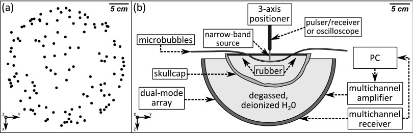
(a) Receiver element distribution. (b) Experimental setup.

2.B. Skull specimens

Four of the human calvaria specimens described in Ref. 80 were used in this study. The skull samples were fixed in 10% buffered formalin for preservation. In order to investigate a range of human skull types, four specimens were chosen to represent thin (Skull A), intermediate (Skull B and Skull D), and thick (Skull C) skulls, as shown in Fig. 2. Each specimen was mounted in a polycarbonate frame, placed in a large plastic container filled with degassed/deionized water, and had previously been imaged with a CT scanner (LightSpeed VCT, GE Healthcare, Chalfont St Giles, UK) using a bone kernel and with an isotropic resolution of 625 × 625 × 625 μm³. The CT scans were used as inputs into the numerical model presented in Sec. 2.F. Table I provides a summary of the average thickness and density values for the skull specimens used in this study.

FIG. 2.

Coronal and sagittal views of the hemispherical array, inner and outer skull surfaces, and source locations investigated for each of the specimens used in this study. The black x’s (circles) indicate locations investigated in the fixed source (tube phantom) experiments.

TABLE I.

Mean (± standard deviation) thickness and density values of the skull specimens used in this study. The values are calculated based on rays from the geometric focus of the array to each of the 128 receiver elements.

Skull	Thickness (mm)	Density (kg m−3)
A	6.1 ± 1.0	1797 ± 85
B	7.5 ± 1.3	1951 ± 196
C	10.2 ± 1.6	1946 ± 86
D	8.0 ± 1.6	1687 ± 91

2.C. Benchtop experiments

The experimental setup is shown in Fig. 1(b). The dual-mode array was filled with degassed/deionized water and was centered below a three-axis positioning system. An ex vivo human skullcap was degassed in a vacuum jar for a minimum of 3 h prior to beginning each experiment and positioned such that its geometric center was approximately coincident with the natural focus of the array (Fig. 2), though the frame attached to the skullcap limited the depth into the dome that it could be placed. A plastic bag was suspended within the skull cavity in order to raise the water level, and rubber absorbers were suspended along the air–water interface in order to mitigate confounding reflections [Fig. 1(b)].

In the first set of benchtop experiments, the fixed source described in Sec. 2.A was mounted to the three-axis positioner and moved around the field to different locations, as shown in Fig. 2. At each point, the fixed source was excited using a broadband impulse from a pulser/receiver (Panametrics, Olympus-NDT, Waltham, MA), and the signals received at each array element were recorded. The source was excited 16 consecutive times and the signals were averaged to improve the signal-to-noise ratio (SNR) of the measured traces. The resulting signals were band-pass filtered (50 kHz–2 MHz passband, fourth order Butterworth, matlab ™), removing high frequency noise and any DC bias. This experiment was conducted with four different skullcaps (Skull A, Skull B, Skull C, and Skull D) placed between the array and the source, for a total of 106 source locations spanning [−50,50] mm in X, [−70,60] mm in Y, and [0,40] mm in Z (Fig. 2).

A second set of benchtop experiments were conducted, where a thin-walled tube phantom was mounted to the three-axis positioner, and a solution of Definity™ microbubbles (Lantheus Medical Imaging, North Billerica, MA) diluted in saline was gravity fed through the tubing (flow rate: 2.1 ml min⁻¹). The polytetrafluoroethylene tubing (Cole-Parmer, Vernon Hills, IL) had an inner and outer diameter of 0.8 and 1.4 mm, respectively. The transmit array was used to excite the microbubbles transcranially, and the resulting acoustic emissions were recorded by the receiver array. Exposures were conducted at various target locations within the skull cavity [Skull B (Fig. 2)] and with varying concentrations of microbubble solution (dilution ratio ranged from 1:1000 to 1:16 000 000). Both single focus sonications and volumetric scans were performed. For volumetric scans, data were captured from the sonications at each transmit focus, and frames containing a single distinct source (peak sidelobe level < − 3 dB) were kept for image reconstruction.⁶¹ Each frame was normalized to itself, and a maximum pixel projection was taken across all remaining frames to generate a complete image of the tube.

Ultrasound transmission through the skull was achieved using geometric focusing only, since at the relatively low driving frequency, skull-induced aberrations are minimal.⁸¹ The transmit array elements were excited with a 5 cycle burst at a pulse repetition frequency (PRF) of 10 Hz using a 128-channel driving system (V-1, Verasonics, Redmond, WA), and the peak negative focal pressure (mechanical index) obtained through the skull was estimated to be 0.11–0.33 MPa (0.19–0.56) in situ, which varied depending on the target location and applied voltage. The pressure at the geometric focus of the array as a function of the driving system input voltage was measured using a calibrated fiber-optic hydrophone (Precision Acoustics, Dorset, UK) without the skull in place. This measurement was then repeated with the 1 mm diameter emitter/receiver used in the fixed source experiments, in order to calibrate the ceramic transducer. The voltage output from the ceramic transducer was measured using an oscilloscope (TDS 3014B, Tektronix, Richardson, TX). In all subsequent measurements with the skull in place, the focal pressure was monitored with the calibrated ceramic transducer. The raw RF data from the receiver array were recorded using a 128-element data acquisition system (SonixDAQ, Ultrasonix, Richmond, BC, Canada)⁸² at a sampling rate between 10 and 40 MS s⁻¹. The speed of sound in water was determined by measuring the water temperature during each experiment⁸³ using a digital thermometer (Extech Instruments, Waltham, MA). The minimum and maximum recorded temperatures were 19.2 and 24.5 °C, respectively, and the inferred speed of sound ranged from 1480 to 1495 m s⁻¹.

2.D. In vivo experiments

Three Wistar rats (male, 162–193 g) were used to assess the technique in vivo. All experiments in this study were approved by Sunnybrook Research Institute’s Animal Care Committee. The experimental protocol was similar to that of a previous study.⁶⁶ The animals were anesthetized via intramuscular injection of a mixture of ketamine (40–50 mg kg⁻¹) and xylazine (10 mg kg⁻¹). Hair on the animals’ heads was removed using an electric razor followed by application of depilatory cream. The animals were laid supine on a platform and their heads were supported by a plastic membrane that was in contact with the water-filled array. Ultrasound gel was used to acoustically couple the animal head to the membrane. The platform with the animal was moved between the array and a 1.5 T MRI (Signa 1.5 T, GE Healthcare, Milwaukee, WI) for treatment planning and monitoring of BBB opening. T₂-weighted images (fast spin echo; relaxation time: 2000 ms; echo time: 60 ms; echo train length: 4; matrix size: 128 × 128; field of view: 6 × 6 cm; slice thickness: 1 mm) were used to select appropriate target locations. All sonications were performed through the intact rat skull and through a human skullcap (Skull B).

A total of four sonications were performed in each animal, each at a different target location. Each sonication consisted of 130, 5 cycle bursts of ultrasound at a driving frequency of 306 kHz with a 1 Hz PRF. In each animal, sonications were performed at four different pressure levels (estimated in situ pressure = 0.24/0.28/0.31/0.33 MPa). The exposure level assigned to a given target location was chosen randomly for each animal. The transmit and receive equipments were the same as those used for the benchtop experiments (see Sec. 2.C). For each target location, an initial sonication was performed without microbubbles to gather baseline signals. Next, a bolus of Definity™ contrast agent (40 μl kg⁻¹) was delivered via a tail vein catheter simultaneous with the beginning of a second sonication. A minimum of 5 min passed between sonications in an animal. The received RF data were captured and stored for further processing. Post-treatment, gadolinium-based contrast-enhanced (200 μl kg⁻¹ Omniscan, GE Healthcare, Milwaukee, WI) T₁-weighted images (fast spin echo; relaxation time: 500 ms; echo time: 10 ms; echo train length: 4; matrix size: 128 × 128; field of view: 6 × 6 cm; slice thickness: 1 mm) were acquired to detect BBB opening.

2.E. Image formation

The data analysis was performed offline in matlab ™ (R2013a, Mathworks, Natick, MA). For the tube phantom and in vivo experiments, reference data taken before the injection of microbubbles were subtracted from data captured with microbubbles in order to suppress reflections off the skull and tubing, enhancing the overall contrast agent signal. The resulting signals were then digitally filtered using a band-pass filter (fourth order Butterworth, matlab ™) with a 400 kHz bandwidth centered about the second harmonic of the driving signal.⁶⁶

Images were formed using a modified version of the beamforming algorithm described in Ref. 48, known as “time exposure acoustics,” which was adapted to include correction terms to account for the acoustic propagation through skull bone.⁷³ First, a grid of points are prescribed over which the image reconstruction will take place. For each grid point r, the received signals from the array are “backpropagated” (i.e., scaled and delayed) as follows:

$${\displaystyle Q_n(\mathbf{r};t)=a_n\cdot {\hat{p}}_n(t+\frac{\Vert {\mathbf{r}}_n-\mathbf{r}\Vert }{c}-s_n)\cdot \Vert {\mathbf{r}}_n-\mathbf{r}\Vert ,}$$ (1)

where ${\hat{p}}_n\left(t\right)$ is a filtered version of p_n(t), the latter representing the time-dependent pressure measured by receiver n located at position r_n, c is the speed of sound in water, a_n and s_n are amplitude and delay correction terms to compensate for skull effects, and ‖r_n − r‖ represents the distance between receiver n and the grid point r. Multiplication by ‖r_n − r‖ accounts for geometric spreading that would occur during acoustic propagation from a point source located at r to a receiver located at r_n. An image is generated by combining the scaled and delayed signals as follows:⁴⁸

$${\displaystyle I\left(\mathbf{r}\right)=\frac{1}{T}{\int }_{t_0}^{t_0+T}\left[\underset{n\ne m}{\sum _{n=1}^N\sum _{m=1}^N}{Q}_n(\mathbf{r};t)\cdot Q_m(\mathbf{r};t)\right]\mathrm{d}t,}$$ (2)

where [t₀, t₀ + T] is the integration window and N is the total number of elements in the array. It is worth noting that in general the skull correction terms ({a_n},{s_n}) are functions of space and frequency. However, for a sufficiently small reconstruction volume and narrow frequency band, they are not expected to vary substantially.⁸⁴ Nevertheless, the use of voxel-specific skull corrections⁷³ may help improve image quality in the future.

Two methods were used to calculate the amplitude and delay terms to correct the aberrating effects induced by the skull bone. The first method, hereafter referred to as source-based corrections, is an invasive method based on comparing the signals received from the fixed source emitter placed at the imaging location of interest with and without the skull in place.^75–77,84 For receiver n, the signals received with and without the skull in place are cross correlated⁸⁵ to determine the delay term (s_n) based on the time-of-flight difference, while the amplitude term (a_n) is given by the ratio of the maximum of the signal envelope received without the skull in place to that received with the skull in place. This apodization approach is analogous to the “amplitude correction” technique described by White et al.,⁸⁶ and by others,⁷⁶ for transcranial focusing of the transmit beam.

The second method, hereafter referred to as CT-based corrections, is a noninvasive method that uses a numerical ultrasound propagation model to simulate the required aberration corrections based on the skull CT morphology and orientation with respect to the array elements.^78,79 The pulse emitted by a “virtual” point source located at the imaging location of interest is numerically propagated through the skull to the array elements, where the received signals are recorded by averaging the pressure over each receiver element’s surface.⁸⁷ The simulation is repeated with the skull removed from the computational domain in order to compute the aberration corrections for the particular location of interest, as described above. Spatial registration of the skull in the simulations was determined by measuring the location of multiple landmarks (Skull A: 7, Skull B: 8, Skull C: 6, and Skull D: 5) on the inner and outer skull surfaces that were easily identifiable in CT image data of the same specimen. For all experiments performed, the mean error in the skull landmark positions after registration was less than 1 mm.

Representative data illustrating skull aberration correction calculations at the geometric focus for one skull are displayed in Fig. 3. In determining the skull delay terms, cross correlation was performed using data from the first five cycles of each pulse. For source location-receiver element pairs where poor transmission through the skull was observed relative to the water-path case (less than 5% transmission, i.e., a_n > 20), the corresponding received signals were omitted from the beamforming process. The simulated signals were resampled to match the sampling frequency of the experimental waveforms (40 MS s⁻¹) prior to cross correlation. Transskull images produced using noninvasive CT-based skull corrections were compared with those obtained through the invasive source-based correction approach, with images formed without skull-specific corrections, and with water-path control images. Images formed with skull delay corrections only [i.e., a_n = 1 ∀ n in Eq. (1)] were also investigated.

FIG. 3.

(a) Illustration of source- and CT-based skull aberration calculations at the array’s geometric focus for Skull B. Measured and simulated signals (f = 516 kHz) captured with and without the skull in place are shown for one receiver element (top row), along with the delayed skull signals (middle row). Envelopes of the aligned signals are shown (bottom row) to demonstrate amplitude correction calculation. (b) Skull amplitude and delay terms for the entire 128-element array. The vertical black line indicates the receiver chosen for the plots in (a).

The time exposure acoustics beamforming algorithm is well suited to parallel computation, since the intensity value of each voxel at a given time can be calculated independently. As such, the reconstruction algorithm was written in the compute unified device architecture (CUDA) graphics processing unit (GPU) platform, following the “parallelization over time” approach outlined in Ref. 88. A typical reconstruction (20 × 20 × 20 mm³ volume, 0.25 × 0.25 × 0.25 mm³ voxel size, 200 sample integration time, 128 elements) took 303 ± 3 ms/frame (mean ± standard deviation, 10 frames) on a single NVIDIA GPU (GeForce GTX Titan, 6 GB memory, 2688 cores), which resulted in more than a 2500-fold speedup compared to a matlab ™ implementation run on a custom-built CPU (857 ± 7 s, 2.0 GHz processor, 32 GB memory, 6 cores). The normalized root-mean-square error⁸⁹ between the GPU and CPU reconstructions was (3.9 ± 0.1) × 10⁻³ (mean ± standard deviation) for the same 10 frames.

2.F. CT-based aberration corrections

A full wave ultrasound propagation model^90–92 was employed to calculate the aberration corrections required for transcranial image formation. Briefly, the model solves the Westervelt equation,⁹³ which can be written as

$${\displaystyle {\nabla }^{2}p-\frac{1}{c^2}\frac{{\partial }^{2}p}{\partial t^2}+\frac{\delta }{c^4}\frac{{\partial }^{3}p}{\partial t^3}+\frac{\beta }{\rho c^4}\frac{{\partial }^2{p}^2}{\partial t^2}-\nabla p\cdot \nabla (ln\rho )=0,}$$ (3)

where p is the acoustic pressure field, and c, δ, β, and ρ represent the local speed of sound, acoustic diffusivity, coefficient of nonlinearity, and density of the propagation medium, respectively. In the particular case of a narrow-band source, the acoustic diffusivity can be written in terms of the attenuation coefficient as δ = 2αc³(2πf)⁻², where f is the excitation frequency.⁹⁴ It is worth noting that c and α represent the speed of sound and attenuation coefficient, respectively, for longitudinal waves. Shear wave propagation is not taken into account in the Westervelt equation. For the purposes of this work, the linearized form of Eq. (3) was solved (i.e., β = 0).

Spatial maps of the material properties within the simulation domain were extracted from the CT images of the skull specimen of interest. First, a map of the effective skull bone density was estimated based on the CT image intensity, acquired in Hounsfield units, assuming a linear dependence.⁹¹ The resulting density maps were manually segmented in matlab ™ via thresholding to identify all voxels corresponding to skull bone. For a given source frequency of interest, maps of the longitudinal speed of sound and attenuation coefficient were generated by interpolating the empirical relations determined in Ref. 80. Voxels within the computational domain not corresponding to skull bone were assigned material parameters to that of water (ρ = 1000 kg m⁻³, α = 0) based on the values presented in Ref. 95, while the speed of sound (c) was determined directly from measurement of the water temperature.⁸³ In addition, triangulated meshes of the skull surfaces were generated from the segmented data, following the procedure outlined in Ref. 73, in order to determine the proximity of each source location to the inner skull surface.

Equation (3) was solved in cylindrical coordinates using a finite-difference time-domain (FDTD) scheme with second- and fourth-order approximations for the temporal and spatial derivatives, respectively.⁹⁰ Sound was introduced into the computational domain through a point source emitter (10-cycle, 40% cosine-tapered pulse⁹⁶ at the frequency of interest), and the super-absorbing layer approach described by Mei and Fang⁹⁷ was applied on the domain boundaries. Spatial discretization (Δh) was set to be Δh = λ/10, where λ is the acoustic wavelength in water. Numerical stability of the model was enforced by selecting the temporal discretization (Δt) such that the Courant–Friedrichs–Lewy (CFL) number⁹⁸ (CFL = c_maxΔtΔh⁻¹) was less than or equal to 0.25, where c_max is the maximum speed of sound in the simulation domain, resulting in 96–98 points/cycle for the skull specimens investigated in this study. The model was implemented using C++ and CUDA, and the simulations were run using the CPU and GPU described in Sec. 2.E. For a source located at the array’s geometric focus, the typical computation time per element was approximately 240–300 s (propagation with and without skull), depending on the source frequency and skull specimen, translating to a total of 8.5–10.5 h for the 128-element array considered in this study (compared to 24–30 h for an implementation written in C++, run on the CPU).

3. RESULTS

Figure 4 shows lateral (Z = 0; top row) and axial (Y = 0; bottom row) contour images obtained from the fixed source emitter placed at the array’s geometric focus. Transskull images generated without, with source-based, and with CT-based skull delay corrections are shown, along with the corresponding water-path control case. When skull corrections are not taken into account during receive beamforming, significant distortions in the reconstructed focal volumes result (i.e., shifted location of maximum intensity, increased sidelobe levels, and general background signal), in comparison to the water-path control case. However, by including skull delay corrections (source- or CT-based) in the reconstruction algorithm, images similar to those of the water-path case are restored, which is consistent with our previous in silico results.⁷³

FIG. 4.

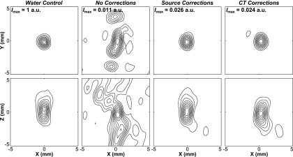
Contour images of the fixed source emitter located at the array’s geometric focus, reconstructed in water, through a human skullcap (Skull C) without skull corrections, with source-based skull delay corrections, and CT-based skull delay corrections. Lateral (Z = 0) and axial (Y = 0) reconstructions are shown. The peak intensity (I_max) for each image is given normalized to the water control case at [0,0,0]. Linear contours are displayed at 10% intervals.

Figure 5 illustrates the dependence of source location on image quality for the various reconstruction methods. Lateral contour planes of image data obtained from the fixed source emitter placed at three different locations spanning 40 mm along the X-axis are plotted for both skull correction techniques, along with the water-path control case. As the source location is moved away from the array’s geometric focus and closer to the inner skull surface, large sidelobes appear in the image generated with CT-based skull delay corrections. In contrast, both the source-based correction and water-path control image quality are less sensitive to source location and skull proximity.

FIG. 5.

Contour images of the fixed source emitter located at [0,0,0], [20,0,0], and [40,0,0] mm. Reconstructions in water and through a human skullcap (Skull C) with source-based and CT-based skull delay corrections. Lateral (Z = 0) reconstructions are shown. The peak intensity (I_max) for each image is given normalized to the water control case at [0,0,0]. Linear contours are displayed at 10% intervals.

Figure 6(a) quantifies the above trends by plotting the image SNR as a function of source location for one skull specimen. The image SNR was defined as the ratio of the main lobe intensity to the standard deviation of the background signal (all voxels located greater than a wavelength from the main lobe intensity peak), as done in Ref. 73. The reconstruction volumes were 20 × 20 × 20 mm³ with a uniform voxel size of 0.25 × 0.25 × 0.25 mm³, centered about the source location. The image SNR was found to decrease as the source location was moved away from the array’s geometric focus. Both skull delay correction techniques provided improvements in image SNR and peak sidelobe ratio (data not shown) compared to the no correction case; however, due to the skull’s high insertion loss,⁶⁸ the image SNR of the water-path control case was not fully restored. The inclusion of skull-specific amplitude corrections produced similar results to phase-only corrections for the invasive source-based technique; however, the CT-based technique performed consistently worse for each image quality metric when amplitude corrections were introduced (Fig. 6). The spatial-dependence of skull aberration corrections in transcranial ultrasound is demonstrated in Fig. 6(b). By considering only skull delay corrections calculated for [0,0,0], and applying these to the received signals from each of the source locations investigated, it can be seen that an improvement from baseline (i.e., no corrections) is only achieved for source locations up to a maximum of 20 mm away from [0,0,0] [Fig. 6(b)], which was the case for each of the four skullcaps investigated.

FIG. 6.

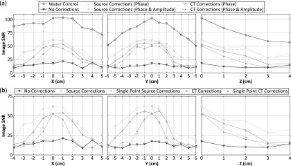
Image SNR as a function of fixed source location. (a) Results from transcranial (Skull C) reconstructions without skull corrections, with source-based and CT-based skull corrections, and water-path control reconstructions. (b) Results from transcranial (Skull C) reconstructions without skull corrections, with skull delay corrections (source- and CT-based) calculated from a single point (chosen to be [0,0,0]), and with location-specific skull delay corrections (source- and CT-based), as presented in (a).

The results from all four skullcaps investigated are summarized in Fig. 7 through different image quality metrics. A positional error with respect to the true source location was observed in the reconstructed images [Fig. 7(a)]. For source locations at least 25 mm from the inner skull surface (62 of 106), this error was 1.4 ± 1.2 mm when the effects of the skull were ignored during image reconstruction. With source-based (CT-based) skull delay corrections, this error was reduced to 0.3 ± 0.2 mm (0.4 ± 0.4 mm). In the absence of skull corrections, the −3 dB volume was found to increase with increasing skull thickness [Fig. 7(b)]. When source-based skull corrections were employed, a single focus was always produced and the mean −3 dB volume was significantly reduced. Multiple foci appeared for a subset of source locations less than 25 mm from the inner skull surface using CT-based corrections. Both skull correction techniques provided improvements in peak sidelobe ratio [Fig. 7(c)] and image SNR [Fig. 7(d)] compared to the no correction case.

FIG. 7.

Summary of the results from all fixed source experiments. The (a) positional error, (b) −3 dB volume, (c) peak sidelobe ratio, and (d) image SNR are plotted (averaged over 62 locations tested at least 25 mm from the inner skull surface, error bars denote one standard deviation) for each transcranial reconstruction case and for the water-path control case. Results for each skullcap investigated are shown, along with a mean value across all skulls.

Figure 8 shows results from a phantom microvessel experiment where the thin-walled tube was fixed near the geometric focus of the array, parallel to the X-axis, and Definity™ microbubbles diluted 1:1000 in saline were flowed through the tube. A volume scan of the tube was performed using electronic steering to scan a 20 × 5 × 12 mm³ volume with a step size of 0.5 mm in X, 1 mm in Y, and 4 mm in Z. The resulting image generated without skull corrections is substantially distorted, with strong signal appearing to originate from outside of the tube. The use of CT-based skull delay corrections led to a larger number of usable frames and resulted in a final compound image with signal confined to the tube region, with a larger portion of the tube visible. The invasive source-based skull correction method restored similar images to those generated using the noninvasive approach.

FIG. 8.

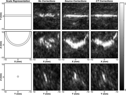
Normalized maximum pixel projection images of the tube phantom, obtained through a human skullcap (Skull B), generated by electronically scanning the transmit focus (grid dimensions: 20 × 5 × 12 mm³; step size: 0.5 mm in X, 1 mm in Y, and 4 mm in Z). Transcranial images formed without skull corrections (n_frames = 9), with source-based skull delay corrections (n_frames = 238), and CT-based (n_frames = 194) skull delay corrections are shown. The cross sectional images (bottom row) were generated by taking the maximum pixel projection within the range of [−1,1] mm in X.

A second experiment was conducted with the phantom microvessel setup, in which the microbubble concentration was decreased to a dilution ratio of 1:16 000 000. At this concentration, assuming a 50% loss of bubbles due to handling,⁹⁹ which is consistent with our previous measurements,⁶⁶ there is approximately 1 bubble per 6 mm of tubing. Compared to the relatively small size of the therapeutic focus (−3 dB lateral width = 3 mm), it is reasonable to expect that the images produced are those of single bubbles.⁶¹ Using data from single bubbles [Fig. 9(a)], the imaging system’s PSF can be estimated [Fig. 9(b)]. It is worth noting that the axial width of the main lobe was found to be approximately twice that of the lateral width, which is consistent with our previous simulations⁷³ and experimental measurements,⁶⁶ and is expected due to the hemispherical element layout. In Fig. 9(b), the measured main lobe beam dimensions, peak sidelobe ratio, and image SNR metrics for ten individual bubbles were compared with the results from corresponding simulations of point source emitters with additive noise from the experimentally measured signals,⁷³ showing good agreement.

FIG. 9.

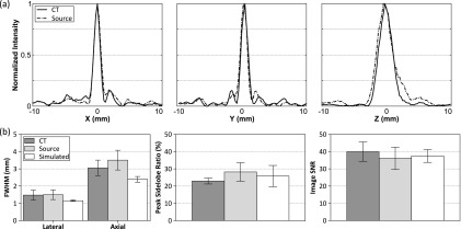
(a) Normalized intensity profiles along the X, Y, and Z directions for a single bubble located near the array’s geometric focus. Transcranial (Skull B) reconstructions with CT- and source-based skull delay corrections are shown. (b) Image quality metrics [full width at half maximum (FWHM), peak sidelobe ratio, image SNR] averaged over ten bubbles are plotted for measured (CT- and source-based skull delay corrections) and simulated data. Error bars denote one standard deviation.

Figure 10 shows results from the in vivo experiments. Representative maps of microbubble activity obtained during ultrasound exposure at pressure levels below and above the threshold for BBB opening are shown [Fig. 10(a)]. For these bursts, the location of maximum intensity in the maps generated without aberration corrections was displaced 2.3 and 7.5 mm, respectively, from the peak location in the maps generated with source-based skull corrections. In both bursts, the peak location in the maps generated with CT-based skull corrections was less than 1 mm from the location obtained with source-based corrections. A contrast-enhanced T₁-weighted MR image of the same rat is shown in Fig. 10(b). Signal enhancement indicating BBB opening is seen at location 2 of the T₁-weighted image. Sonications at the two highest pressures (0.31/0.33 MPa) resulted in BBB opening in all six cases, whereas no BBB opening was observed at either of the lowest two pressures (0.24/0.28 MPa). Summarizing the data from all sonications (Table II), it was found that during bursts that led to coherent bubble activity (peak sidelobe ratio < − 3 dB; 416/1560 bursts), without skull corrections the mean location of maximum intensity was displaced 2.3 ± 2.0 mm from the position obtained using source-based corrections, whereas with CT-based corrections this shift was reduced to 0.8 ± 0.5 mm.

FIG. 10.

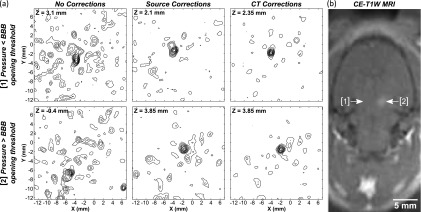
(a) Maps of microbubble activity generated in a rat model through an ex vivo human skullcap (Skull B) during FUS exposure at pressure levels below (location 1; estimated in situ pressure = 0.24 MPa) and above (location 2; 0.33 MPa) the threshold for BBB opening. Lateral planes of maximum intensity are shown for reconstructions with no skull corrections and with source- and CT-based skull delay corrections. Linear contours are displayed at 10% intervals. (b) Contrast-enhanced T₁-weighted (CE-T1W) MR image of the same rat postsonication showing enhancement at sonication location 2. The sonication direction is into the page.

TABLE II.

Summary of results from the in vivo experiments. The distance between the location of maximum intensity (mean ± standard deviation) in images (peak sidelobe ratio < − 3 dB) generated without corrections and with CT-based skull delay corrections relative to the peak location in the source-based correction case (Δ_no and Δ_CT, respectively) is shown for all four sonications in each rat. The number of frames with “coherent bubble activity” (peak sidelobe ratio < − 3 dB) during each sonication is also listed (n_frames).

Rat	Metric	0.24 MPa	0.28 MPa	0.31 MPa	0.33 MPa	All
	ΔCT	0.6 ± 0.4	0.8 ± 0.4	N/A	0.8 ± 0.6	0.7 ± 0.5
1	Δno	1.8 ± 1.1	1.4 ± 1.7	N/A	2.1 ± 0.5	1.8 ± 1.2
	nframes	101/130	62/130	0/130	63/130	226/520
	ΔCT	0.8 ± 0.6	0.7 ± N/A	1.1 ± 0.5	0.5 ± 0.2	0.9 ± 0.6
2	Δno	3.4 ± 4.5	1.9 ± N/A	2.1 ± 0.5	6.1 ± 2.3	3.1 ± 2.7
	nframes	22/130	1/130	75/130	26/130	124/520
	ΔCT	0.2 ± N/A	0.7 ± 0.4	0.9 ± 0.5	N/A	0.7 ± 0.4
3	Δno	2.5 ± N/A	2.3 ± 2.2	2.3 ± 2.4	N/A	2.3 ± 2.2
	nframes	1/130	60/130	5/130	0/130	66/520
	ΔCT	0.6 ± 0.4	0.7 ± 0.4	1.1 ± 0.5	0.7 ± 0.6	0.8 ± 0.5
All	Δno	2.0 ± 2.2	1.9 ± 2.0	2.1 ± 0.8	3.3 ± 2.3	2.3 ± 2.0
	nframes	124/390	123/390	80/390	89/390	416/1560

4. DISCUSSION

The results of this study confirm that the proposed method is capable of compensating for the aberrating effects of the skull and enable transcranial mapping of microbubble cavitation activity in a noninvasive manner. In the future, the information inferred regarding the acoustic activity within the entire skull cavity could be incorporated into existing treatment control schemes³⁵ in order to select optimal sonication parameters such that a desired level of cavitation activity is reached within the target volume. Apart from its use in a therapy monitoring context, since the microbubbles are confined to the vasculature until clearance by the lungs and kidneys, the method could also be combined with super-resolution techniques^61,114,115 to enable vascular mapping of the brain for diagnostic purposes.

Dynamic beam focusing using measurements of the ultrasound field from a reference point, different from the focal location, was investigated in the context of passive imaging through the skull bone [Fig. 6(b)]. Previous studies have investigated the range of validity of this approach for transmit beam focusing through heterogeneous media.^84,100,116 Using an 810 kHz, 120-element phased array (circular discs, 19 mm diameter), Clement and Hynynen measured a 24 mm radial steering range (50% intensity drop-off) when focusing through an ex vivo human skull.⁸⁴ In an earlier study, VanBaren et al. focused a 500 kHz, 64-element cylindrical-section array (rectangular elements, 3 × 150 mm²) through a rubber abberator and found that any attempt to focus beyond 20 mm from the reference point led to a degradation in focal quality.¹⁰⁰ With our system, improvements in image quality (i.e., image SNR) relative to the no correction case were found for all locations 10 mm from the reference point ([0,0,0]) and for 70% of the locations with a separation of 20 mm, while for locations 30 mm and farther from the reference point, no substantial changes from baseline were observed. These results suggest that this approach is valid over a similar range on receive as it has been found to be on transmit, though it is worth noting that this range is highly dependent on the specific array geometry and operating frequency employed.

Results from the in vivo experiments demonstrated the feasibility of mapping microbubble activity in the brain through a human skull. Images of bubble activity were obtained starting at pressure levels below the threshold for BBB opening, which is consistent with our previous results obtained without the presence of a human skull.⁶⁶ Although the technique was applied during FUS-induced BBB opening in the present work, the method is directly applicable to other cavitation-mediated brain therapies, such as ultrasound-assisted clot lysis,^24,25 tissue fractionation,^26,27 or cavitation-enhanced ablation.^101–103 Furthermore, the proposed technology could be used to confirm the absence of inertial cavitation during thermal ablation therapies in the brain, in order to avoid hemorrhagic events.^104,105

Potential sources of error when applying simulation-based methods for transcranial aberration correction include registration (i.e., orientation of skull with respect to transducer array elements) as well as modeling errors. In this study, registration was performed by measuring a handful of landmarks on the inner and outer skull surfaces in the reference frame of the array elements and locating their corresponding voxels in the CT dataset of the same specimen. This process led to a registration error on the order of 1 mm. Although this is a non-negligible fraction of the wavelength at the frequencies investigated in this study (≈0.4 λ), it is worth noting that this misregistration would be reduced in a clinical setting, where the patient’s entire pretreatment CT dataset would be registered to a corresponding MR dataset taken while the patient was stereotactically fixed to the FUS device.

The transcranial propagation model used in this study supports only longitudinal propagation in the skull bone. In the future, the use of more complex models incorporating shear-wave propagation^106–108 or higher order numerical approaches^109,110 may improve aberration correction, particularly at source locations close to the inner skull surface where the angles of incidence are such that significant mode conversion is present. Indeed, our use of a model that neglects shear wave propagation may explain the increased sensitivity of CT-based correction image quality to skull proximity observed in this study (Fig. 5), though further investigations are required in order to confirm this. These approaches will first require that the acoustical properties for shear wave propagation in skull bone as a function of density and frequency be accurately determined. On the other hand, more simplistic and computationally efficient models could also be employed,^78,111–113 in order to reduce treatment planning times. Furthermore, mapping of low-frequency cavitation activity in the brain may be possible without skull-specific corrections,⁷³ due to the diminished aberrations present with longer acoustic wavelengths.⁸¹

Apart from the mechanics of the numerical model, the acoustic parameters used in the simulation domain must also be accurately replicated. In this study, the longitudinal acoustical parameters of skull bone at our frequencies of interest (516 kHz for fixed source experiments and 612 kHz for microbubble mapping) were estimated by interpolating empirical datasets obtained at different frequencies (f_low = 270 kHz and f_high = 836 kHz).⁸⁰ Although the longitudinal sound speed of skull bone has been shown to be relatively constant over this frequency range, the attenuation varies substantially.⁸⁰ This interpolation is likely the reason that the CT-based amplitude and phase corrected images performed worse than phase corrections only, and it is expected that amplitude corrections calculated from data at the appropriate frequency would improve the sidelobe structure and focal quality (i.e., image SNR) compared to phase-only corrections, as is the case on transmit.⁸⁶

Finally, another limitation of this study is that skullcaps were used as opposed to full human skull specimens. Although it is unclear exactly how reflections off of the skull bone will impact the reconstructed images, they are expected to have an effect, particularly when longer pulse lengths are used. Despite the outstanding issues with the method, it is worth noting that clinical implementation of this technique would be simplified by the fact that CT-based skull corrections are already required for transmit focusing.

5. CONCLUSION

This study demonstrates that patient-specific aberration corrections obtained using a numerical ultrasound propagation model combined with CT-derived cranial morphology enable passive imaging of acoustic sources through the intact human skull in a noninvasive manner. The technique was shown to be capable of transcranially imaging a narrow-band fixed source, as well as ultrasound-stimulated microbubbles in microvessel-mimicking tube phantoms and in a rat model of BBB opening. Based on the results of this noninvasive approach, we conclude that the reconstruction algorithm may be useful for the monitoring and control of FUS treatments in the brain, particularly microbubble-mediated applications, in order to improve therapeutic safety and efficacy. Additionally, the method may also have application in ultrasound-based vascular imaging in the brain. Future work in this area will concentrate on comprehensive in vivo testing of the technique, along with further algorithm development with a view toward improving the imageable volume within the skull cavity.

REFERENCES

- 1.Elias W. J., Huss D., Voss T., Loomba J., Khaled M., Zadicario E., Frysinger R. C., Sperling S. A., Wylie S., Monteith S. J., Druzgal J., Shah B. B., Harrison M., and Wintermark M., “A pilot study of focused ultrasound thalamotomy for essential tremor,” N. Engl. J. Med. 369, 640–648 (2013). 10.1056/NEJMoa1300962 [DOI] [PubMed] [Google Scholar]
- 2.Lipsman N., Shwartz M. L., Huang Y., Lee L., Sankar T., Chapman M., Hynynen K., and Lozano A. M., “MR-guided focused ultrasound thalamotomy for essential tremor: A proof-of-concept study,” Lancet Neurol. 12, 462–468 (2013). 10.1016/S1474-4422(13)70048-6 [DOI] [PubMed] [Google Scholar]
- 3.Heimburger R. F., “Ultrasound augmentation of central nervous system tumor therapy,” Indiana Med. 78, 469–476 (1985). [PubMed] [Google Scholar]
- 4.Ram Z., Cohen Z. R., Harnof S., Tal S., Faibel M., Nass D., Maier S. E., Hadani M., and Mardor Y., “Magnetic resonance imaging-guided, high-intensity focused ultrasound for brain tumor therapy,” Neurosurgery 59, 949–956 (2006). [DOI] [PubMed] [Google Scholar]
- 5.McDannold N., Clement G. T., Black P., Jolesz F., and Hynynen K., “Transcranial magnetic resonance imaging-guided focused ultrasound surgery of brain tumors: Initial findings in 3 patients,” Neurosurgery 66, 323–332 (2010). 10.1227/01.NEU.0000360379.95800.2F [DOI] [PMC free article] [PubMed] [Google Scholar]
- 6.Coluccia D., Fandino J., Schwyzer L., O’Gorman R., Remonda L., Anon J., Martin E., and Werner B., “First noninvasive thermal ablation of a brain tumor with MR-guided focused ultrasound,” J. Ther. Ultrasound 2, 17 (7pp.) (2014). 10.1186/2050-5736-2-17 [DOI] [PMC free article] [PubMed] [Google Scholar]
- 7.Martin E., Jeanmonod D., Morel A., Zadicario E., and Werner B., “High-intensity focused ultrasound for noninvasive functional neurosurgery,” Ann. Neurol. 66, 858–861 (2009). 10.1002/ana.21801 [DOI] [PubMed] [Google Scholar]
- 8.Jeanmonod D., Werner B., Model A., Michels L., Zadicario E., Schiff G., and Martin E., “Transcranial magnetic resonance imaging-guided focused ultrasound: Noninvasive central lateral thalamotomy for chronic neuropathic pain,” Neurosurg. Focus 32, E1 (11pp.) (2012). 10.3171/2011.10.FOCUS11248 [DOI] [PubMed] [Google Scholar]
- 9.Fry W. J. and Fry F. J., “Fundamental neurological research and human neurosurgery using intense ultrasound,” IRE Trans. Med. Electron. ME-7, 166–181 (1960). 10.1109/IRET-ME.1960.5008041 [DOI] [PubMed] [Google Scholar]
- 10.Magara A., Bühler R., Moser D., Kowalski M., Pourtehrani P., and Jeanmonod D., “First experience with MR-guided focused ultrasound in the treatment of Parkinson’s disease,” J. Ther. Ultrasound 2, 11 (8pp.) (2014). 10.1186/2050-5736-2-11 [DOI] [PMC free article] [PubMed] [Google Scholar]
- 11.Jung H. H., Kim S. J., Roh D., Chang J. G., Chang W. S., Kweon E. J., Kim C.-H., and Chang J. W., “Bilateral thermal capsulotomy with MR-guided focused ultrasound for patients with treatment-refractory obsessive-compulsive disorder: A proof-of-concept study,” Mol. Psychiatry (2014) [E-pub ahead of print]. 10.1038/mp.2014.154 [DOI] [PubMed] [Google Scholar]
- 12.Lipsman N., Mainprize T. G., Schwartz M. L., Hynynen K., and Lozano A. M., “Intracranial applications of magnetic resonance-guided focused ultrasound,” Neurotherapeutics 11, 593–605 (2014). 10.1007/s13311-014-0281-2 [DOI] [PMC free article] [PubMed] [Google Scholar]
- 13.Hynynen K., Vykhodtseva N. I., Chung A. H., Sorrentino V., Colucci V., and Jolesz F. A., “Thermal effects of focused ultrasound on the brain: Determination with MR imaging,” Radiology 204, 247–253 (1997). 10.1148/radiology.204.1.9205255 [DOI] [PubMed] [Google Scholar]
- 14.Ishihara Y., Calderon A., Watanabe H., Okamoto K., Suzuki Y., Kuroda K., and Suzuki Y., “A precise and fast temperature mapping using water proton chemical shift,” Magn. Reson. Med. 34, 814–823 (1995). 10.1002/mrm.1910340606 [DOI] [PubMed] [Google Scholar]
- 15.De Poorter J., De Wagter C., De Deene Y., Thomsen C., Ståhlberg F., and Achten E., “Noninvasive MRI thermometry with the proton resonance frequency (PRF) method: in vivo results in human muscle,” Magn. Reson. Med. 33, 74–81 (1995). 10.1002/mrm.1910330111 [DOI] [PubMed] [Google Scholar]
- 16.Hindman J. C., “Proton resonance shift of water in the gas and liquid states,” J. Chem. Phys. 44, 4582–4592 (1966). 10.1063/1.1726676 [DOI] [Google Scholar]
- 17.Hynynen K., McDannold N., Vykhodtseva N., and Jolesz F. A., “Noninvasive MR imaging-guided focal opening of the blood-brain barrier in rabbits,” Radiology 220, 640–646 (2001). 10.1148/radiol.2202001804 [DOI] [PubMed] [Google Scholar]
- 18.Choi J. J., Pernot M., Small S. A., and Konofagou E. E., “Noninvasive, transcranial and localized opening of the blood-brain barrier using focused ultasound in mice,” Ultrasound Med. Biol. 33, 95–104 (2007). 10.1016/j.ultrasmedbio.2006.07.018 [DOI] [PubMed] [Google Scholar]
- 19.Liu H.-L., Hua M.-Y., Chen P.-Y., Chu P.-C., Pan C.-H., Yang H.-W., Huang C.-Y., Wang J.-J., Yen T.-C., and Wei K.-C., “Blood-brain barrier disruption with focused ultrasound enhances delivery of chemotherapeutic drugs for glioblastoma treatment,” Radiology 255, 415–425 (2010). 10.1148/radiol.10090699 [DOI] [PubMed] [Google Scholar]
- 20.McDannold N., Arvanitis C. D., Vykhodtseva N., and Livingstone M. S., “Temporary disruption of the blood-brain barrier by use of ultrasound and microbubbles: Safety and efficacy evaluation in rhesus macaques,” Cancer Res. 72, 3652–3663 (2012). 10.1158/0008-5472.CAN-12-0128 [DOI] [PMC free article] [PubMed] [Google Scholar]
- 21.Aryal M., Vykhodtseva N., Zhang Y.-Z., Park J., and McDannold N., “Multiple treatments with liposomal doxorubicin and ultrasound-induced disruption of blood-tumor and blood-brain barriers improve outcomes in a rat glioma model,” J. Control. Release 169, 103–111 (2013). 10.1016/j.jconrel.2013.04.007 [DOI] [PMC free article] [PubMed] [Google Scholar]
- 22.Trübestein G., Engel C., Etzel F., Sobbe A., Cremer H., and Stumpff U., “Thrombolysis by ultrasound,” Clin. Sci. Mol. Med., Suppl. 3, 697s–698s (1976). [DOI] [PubMed] [Google Scholar]
- 23.Tachibana K. and Tachibana S., “Albumin microbubble echo-contrast material as an enhancer for ultrasound accelerated thrombolysis,” Circulation 92, 1148–1150 (1995). 10.1161/01.CIR.92.5.1148 [DOI] [PubMed] [Google Scholar]
- 24.Culp W. C., Flores R., Brown A. T., Lowery J. D., Roberson P. K., Hennings L. J., Woods S. D., Hatton J. H., Culp B. C., Skinner R. D., and Borrelli M. J., “Successful microbubble sonothrombolysis without tissue-type plasminogen activator in a rabbit model of acute ischemic stroke,” Stroke 42, 2280–2285 (2011). 10.1161/STROKEAHA.110.607150 [DOI] [PMC free article] [PubMed] [Google Scholar]
- 25.Burgess A., Huang Y., Waspe A. C., Ganguly M., Goertz D. E., and Hynynen K., “High-intensity focused ultrasound (HIFU) for dissolution of clots in a rabbit model of embolic stroke,” PLoS One 7, e42311 (2012). 10.1371/journal.pone.0042311 [DOI] [PMC free article] [PubMed] [Google Scholar]
- 26.Alkins R., Huang Y., Pajek D., and Hynynen K., “Cavitation-based third ventriculostomy using MRI-guided focused ultrasound,” J. Neurosurg. 119, 1520–1529 (2013). 10.3171/2013.8.JNS13969 [DOI] [PMC free article] [PubMed] [Google Scholar]
- 27.Kim Y., Hall T. L., Xu Z., and Cain C. A., “Transcranial histotripsy therapy: A feasibility study,” IEEE Trans. Ultrason. Ferroelectr. Freq. Control 61, 582–593 (2014). 10.1109/TUFFC.2014.2947 [DOI] [Google Scholar]
- 28.Noltingk B. E. and Neppiras E. A., “Cavitation produced by ultrasonics,” Proc. Phys. Soc., Sect. B 63, 674–685 (1950). 10.1088/0370-1301/63/9/305 [DOI] [Google Scholar]
- 29.Feinstein S. B., Shah P. M., Bing R. J., Meerbaum S., Corday E., Chang B.-L., Santillan G., and Fujibayashi Y., “Microbubble dynamics visualized in the intact capillary circulation,” J. Am. Coll. Cardiol. 4, 595–600 (1984). 10.1016/S0735-1097(84)80107-2 [DOI] [PubMed] [Google Scholar]
- 30.Calliada F., Campani R., Bottinelli O., Bozzini A., and Sommaruga M. G., “Ultrasound contrast agents: Basic principles,” Eur. J. Radiol. 27, S157–S160 (1998). 10.1016/S0720-048X(98)00057-6 [DOI] [PubMed] [Google Scholar]
- 31.Fatar M., Stroick M., Griebe M., Alonso A., Hennerici M. G., and Daffertshofer M., “Brain temperature during 340-kHz pulsed ultrasound insonation: A safety study for sonothrombolysis,” Stroke 37, 1883–1887 (2006). 10.1161/01.STR.0000226737.47319.aa [DOI] [PubMed] [Google Scholar]
- 32.McDannold N., Vykhodtseva N., and Hynynen K., “Targeted disruption of the blood-brain barrier with focused ultrasound: Association with cavitation activity,” Phys. Med. Biol. 51, 793–807 (2006). 10.1088/0031-9155/51/4/003 [DOI] [PubMed] [Google Scholar]
- 33.Tung Y.-S., Vlachos F., Choi J. J., Deffieux T., Selert K., and Konofagou E. E., “In vivo transcranial cavitation threshold detection during ultrasound-induced blood-brain barrier opening in mice,” Phys. Med. Biol. 55, 6141–6155 (2010). 10.1088/0031-9155/55/20/007 [DOI] [PMC free article] [PubMed] [Google Scholar]
- 34.Tung Y.-S., Marquet F., Teichert T., Ferrera V., and Konofagou E. E., “Feasibility of noninvasive cavitation-guided blood-brain barrier opening using focused ultrasound and microbubbles in nonhuman primates,” Appl. Phys. Lett. 98, 163704 (2011). 10.1063/1.3580763 [DOI] [PMC free article] [PubMed] [Google Scholar]
- 35.O’Reilly M. A. and Hynynen K., “Blood-brain barrier: Real-time feedback-controlled focused ultrasound disruption by using an acoustic emissions-based controller,” Radiology 263, 96–106 (2012). 10.1148/radiol.11111417 [DOI] [PMC free article] [PubMed] [Google Scholar]
- 36.Arvanitis C. D., Livingstone M. S., Vykhodtseva N., and McDannold N., “Controlled ultrasound-induced blood-brain barrier disruption using passive acoustic emissions monitoring,” PLoS One 7, e45783 (2012). 10.1371/journal.pone.0045783 [DOI] [PMC free article] [PubMed] [Google Scholar]
- 37.Wu S.-Y., Tung Y.-S., Marquet F., Downs M. E., Sanchez C. S., Chen C. C., Ferrera V., and Konofagou E., “Transcranial cavitation detection in primates during blood-brain barrier opening-a performance assessment study,” IEEE Trans. Ultrason. Ferroelectr. Freq. Control 61, 966–978 (2014). 10.1109/TUFFC.2014.2992 [DOI] [PMC free article] [PubMed] [Google Scholar]
- 38.Datta S., Coussios C.-C., McAdory L. E., Tan J., Porter T., De Courten-Myers G., and Holland C. K., “Correlation of cavitation with ultrasound enhancement of thrombolysis,” Ultrasound Med. Biol. 32, 1257–1267 (2006). 10.1016/j.ultrasmedbio.2006.04.008 [DOI] [PMC free article] [PubMed] [Google Scholar]
- 39.Prokop A. F., Soltani A., and Roy R. A., “Cavitational mechanisms in ultrasound-accelerated fibrinolysis,” Ultrasound Med. Biol. 33, 924–933 (2007). 10.1016/j.ultrasmedbio.2006.11.022 [DOI] [PubMed] [Google Scholar]
- 40.Datta S., Coussios C.-C., Ammi A. Y., Mast T. D., de Courten-Myers G. M., and Holland C. K., “Ultrasound-enhanced thrombolysis using Definity® as a cavitation nucleation agent,” Ultrasound Med. Biol. 34, 1421–1433 (2008). 10.1016/j.ultrasmedbio.2008.01.016 [DOI] [PMC free article] [PubMed] [Google Scholar]
- 41.Wright C., Hynynen K., and Goertz D., “In vitro and in vivo high-intensity focused ultrasound thrombolysis,” Invest. Radiol. 47, 217–225 (2012). 10.1097/RLI.0b013e31823cc75c [DOI] [PMC free article] [PubMed] [Google Scholar]
- 42.Leeman J. E., Kim J. S., Yu F. T. H., Chen X., Kim K., Wang J., Chen X., Villaneuva F. S., and Pacella J. J., “Effect of acoustic conditions on microbubble-mediated microvascular sonothrombolysis,” Ultrasound Med. Biol. 38, 1589–1598 (2012). 10.1016/j.ultrasmedbio.2012.05.020 [DOI] [PubMed] [Google Scholar]
- 43.Xu Z., Fowlkes J. B., Rothman E. D., Levin A. M., and Cain C. A., “Controlled ultrasound tissue erosion: The role of dynamic interaction between insonation and microubbble activity,” J. Acoust. Soc. Am. 117, 424–435 (2005). 10.1121/1.1828551 [DOI] [PMC free article] [PubMed] [Google Scholar]
- 44.Parsons J. E., Cain C. A., Abrams G. D., and Fowlkes J. B., “Pulsed cavitational ultrasound therapy for controlled tissue homogenization,” Ultrasound Med. Biol. 32, 115–129 (2006). 10.1016/j.ultrasmedbio.2005.09.005 [DOI] [PubMed] [Google Scholar]
- 45.Wolf E. and Shewell J. R., “The inverse wave propagator,” Phys. Lett. A 25, 417–418 (1967). 10.1016/0375-9601(67)90056-4 [DOI] [Google Scholar]
- 46.Sato T., Uemura K., and Sasaki K., “Super-resolution acoustical passive system using algebraic reconstruction,” J. Acoust. Soc. Am. 67, 1802–1808 (1980). 10.1121/1.384257 [DOI] [Google Scholar]
- 47.Troitskiy P., Husebye E. S., and Nikolaev A., “Lithospheric studies based on holographic principles,” Nature 294, 618–623 (1981). 10.1038/294618a0 [DOI] [Google Scholar]
- 48.Norton S. J. and Won I. J., “Time exposure acoustics,” IEEE Trans. Geosci. Remote Sens. 38, 1337–1343 (2000). 10.1109/36.843027 [DOI] [Google Scholar]
- 49.Gyöngy M., Arora M., Noble J. A., and Coussios C. C., “Use of passive arrays for characterization and mapping of cavitation activity during HIFU exposure,” Proc. IEEE Ultrason. Symp. 871–874 (2008). 10.1109/ULTSYM.2008.0210 [DOI] [Google Scholar]
- 50.Salgaonkar V. A., Datta S., Holland C. K., and Mast T. D., “Passive cavitation imaging with ultrasound arrays,” J. Acoust. Soc. Am. 126, 3071–3083 (2009). 10.1121/1.3238260 [DOI] [PMC free article] [PubMed] [Google Scholar]
- 51.Farny C. H., Holt R. G., and Roy R. A., “Temporal and spatial detection of HIFU-induced inertial and hot-vapor cavitation with a diagnostic ultrasound system,” Ultrasound Med. Biol. 35, 603–615 (2009). 10.1016/j.ultrasmedbio.2008.09.025 [DOI] [PubMed] [Google Scholar]
- 52.Gyöngy M. and Coussios C.-C., “Passive spatial mapping of inertial cavitation during HIFU exposure,” IEEE Trans. Biomed. Eng. 57, 48–56 (2010). 10.1109/TBME.2009.2026907 [DOI] [PubMed] [Google Scholar]
- 53.Gyöngy M. and Coussios C.-C., “Passive cavitation mapping for localization and tracking of bubble dynamics,” J. Acoust. Soc. Am. 128, EL175–EL180 (2010). 10.1121/1.3467491 [DOI] [PubMed] [Google Scholar]
- 54.Gyöngy M. and Coviello C. M., “Passive cavitation mapping with temporal sparsity constraint,” J. Acoust. Soc. Am. 130, 3489–3497 (2011). 10.1121/1.3626138 [DOI] [PubMed] [Google Scholar]
- 55.Gateau J., Aubry J.-F., Pernot M., Fink M., and Tanter M., “Combined passive detection and ultrafast active imaging of cavitation events induced by short pulses of high-intensity ultrasound,” IEEE Trans. Ultrason. Ferroelectr. Freq. Control 58, 517–532 (2011). 10.1109/TUFFC.2011.1836 [DOI] [PMC free article] [PubMed] [Google Scholar]
- 56.Coviello C. M., Kozick R. J., Hurrell A., Smith P. P., and Coussios C.-C., “Thin-film sparse boundary array design for passive acoustic mapping during ultrasound therapy,” IEEE Trans. Ultrason. Ferroelectr. Freq. Control 59, 2322–2330 (2012). 10.1109/tuffc.2012.2457 [DOI] [PubMed] [Google Scholar]
- 57.Choi J. J. and Coussios C.-C., “Spatiotemporal evolution of cavitation dynamics exhibited by flowing microbubbles during ultrasound exposure,” J. Acoust. Soc. Am. 132, 3538–3549 (2012). 10.1121/1.4756926 [DOI] [PubMed] [Google Scholar]
- 58.Haworth K. J., Mast T. D., Radhakrishnan K., Burgess M. T., Kopechek J. A., Huang S.-L., McPherson D. D., and Holland C. K., “Passive imaging with pulsed ultrasound insonations,” J. Acoust. Soc. Am. 132, 544–553 (2012). 10.1121/1.4728230 [DOI] [PMC free article] [PubMed] [Google Scholar]
- 59.Jensen C. R., Ritchie R. W., Gyöngy M., Collin J. R. T., Leslie T., and Coussios C.-C., “Spatiotemporal monitoring of high-intensity focused ultrasound therapy with passive acoustic mapping,” Radiology 262, 252–261 (2012). 10.1148/radiol.11110670 [DOI] [PubMed] [Google Scholar]
- 60.Jensen C. R., Cleveland R. O., and Coussios C. C., “Real-time temperature estimation and monitoring of HIFU ablation through a combined modeling and passive acoustic mapping approach,” Phys. Med. Biol. 58, 5833–5850 (2013). 10.1088/0031-9155/58/17/5833 [DOI] [PubMed] [Google Scholar]
- 61.O’Reilly M. A. and Hynynen K., “A super-resolution ultrasound method for brain vascular mapping,” Med. Phys. 40, 110701(7pp.) (2013). 10.1118/1.4823762 [DOI] [PMC free article] [PubMed] [Google Scholar]
- 62.Pouliopoulos A. N., Bonaccorsi S., and Choi J. J., “Exploiting flow to control the in vitro spatiotemporal distribution of microubbble-seeded acoustic cavitation activity in ultrasound therapy,” Phys. Med. Biol. 59, 6941–6957 (2014). 10.1088/0031-9155/59/22/6941 [DOI] [PubMed] [Google Scholar]
- 63.Vignon F., Shi W. T., Powers J. E., Everbach E. C., Liu J., Gao S., Xie F., and Porter T. R., “Microbubble cavitation imaging,” IEEE Trans. Ultrason. Ferroelectr. Freq. Control 60, 661–670 (2013). 10.1109/TUFFC.2013.2615 [DOI] [PMC free article] [PubMed] [Google Scholar]
- 64.Arvanitis C. D. and McDannold N., “Integrated ultrasound and magnetic resonance imaging for simultaneous temperature and cavitation monitoring during focused ultrasound therapies,” Med. Phys. 40, 112901(14pp.) (2013). 10.1118/1.4823793 [DOI] [PMC free article] [PubMed] [Google Scholar]
- 65.Arvanitis C. D., Livingstone M. S., and McDannold N., “Combined ultrasound and MR imaging to guide focused ultrasound therapies in the brain,” Phys. Med. Biol. 58, 4749–4761 (2013). 10.1088/0031-9155/58/14/4749 [DOI] [PMC free article] [PubMed] [Google Scholar]
- 66.O’Reilly M. A., Jones R. M., and Hynynen K., “Three-dimensional transcranial ultrasound imaging of microbubble clouds using a sparse hemispherical array,” IEEE Trans. Biomed. Eng. 61, 1285–1294 (2014). 10.1109/TBME.2014.2300838 [DOI] [PMC free article] [PubMed] [Google Scholar]
- 67.Choi J. J., Carlisle R. C., Coviello C., Seymour L., and Coussios C.-C., “Non-invasive and real-time passive acoustic mapping of ultrasound-mediated drug delivery,” Phys. Med. Biol. 59, 4861–4877 (2014). 10.1088/0031-9155/59/17/4861 [DOI] [PubMed] [Google Scholar]
- 68.Fry F. J. and Barger J. E., “Acoustical properties of the human skull,” J. Acoust. Soc. Am. 63, 1576–1590 (1978). 10.1121/1.381852 [DOI] [PubMed] [Google Scholar]
- 69.Aaslid R., Markwalder T.-M., and Nornes H., “Noninvasive transcranial Doppler ultrasound recording of flow velocity in basal cerebral arteries,” J. Neurosurg. 57, 769–774 (1982). 10.3171/jns.1982.57.6.0769 [DOI] [PubMed] [Google Scholar]
- 70.Kirkham F. J., Padayachee T. S., Parsons S., Seargeant L. S., House F. R., and Gosling R. G., “Transcranial measurement of blood velocities in the basal cerebral arteries using pulsed Doppler ultrasound: Velocity as an index of flow,” Ultrasound Med. Biol. 12, 15–21 (1986). 10.1016/0301-5629(86)90139-0 [DOI] [PubMed] [Google Scholar]
- 71.Smith S. W., Chu K., Idriss S. F., Ivancevich N. M., Light E. D., and Wolf P. D., “Feasibility study: Real-time 3-D ultrasound imaging of the brain,” Ultrasound Med. Biol. 30, 1365–1371 (2004). 10.1016/j.ultrasmedbio.2004.08.012 [DOI] [PubMed] [Google Scholar]
- 72.Lindsey B. D., Nicoletto H. A., Bennett E. R., Laskowitz D. T., and Smith S. W., “Simultaneous bilateral real-time 3-D transcranial ultrasound imaging at 1 MHz through poor acoustic windows,” Ultrasound Med. Biol. 39, 721–734 (2013). 10.1016/j.ultrasmedbio.2012.11.019 [DOI] [PMC free article] [PubMed] [Google Scholar]
- 73.Jones R. M., O’Reilly M. A., and Hynynen K., “Transcranial passive acoustic mapping with hemispherical sparse arrays using CT-based skull-specific aberration corrections: A simulation study,” Phys. Med. Biol. 58, 4981–5005 (2013). 10.1088/0031-9155/58/14/4981 [DOI] [PMC free article] [PubMed] [Google Scholar]
- 74.Song J. and Hynynen K., “Feasibility of using lateral mode coupling method for a large scale ultrasound phased array for noninvasive transcranial therapy,” IEEE Trans. Biomed. Eng. 57, 124–133 (2010). 10.1109/TBME.2009.2028739 [DOI] [PMC free article] [PubMed] [Google Scholar]
- 75.Smith S. W., Phillips D. J., von Ramm O. T., and Thurstone F. L., “Some advances in acoustic imaging through skull,” in Ultrasonic Tissue Characterization II, NSB Publication No. 525 , edited byLinzer M. (U.S. GPO, Washington, DC, 1979), pp. 209–218. [Google Scholar]
- 76.Thomas J.-L. and Fink M. A., “Ultrasonic beam focusing through tissue inhomogeneities with a time reversal mirror: application to transskull therapy,” IEEE Trans. Ultrason. Ferroelectr. Freq. Control 43, 1122–1129 (1996). 10.1109/58.542055 [DOI] [Google Scholar]
- 77.Hynynen K. and Jolesz F. A., “Demonstration of potential noninvasive ultrasound brain therapy through an intact skull,” Ultrasound Med. Biol. 24, 275–283 (1998). 10.1016/S0301-5629(97)00269-X [DOI] [PubMed] [Google Scholar]
- 78.Clement G. T. and Hynynen K., “A non-invasive method for focusing ultrasound through the human skull,” Phys. Med. Biol. 47, 1219–1236 (2002). 10.1088/0031-9155/47/8/301 [DOI] [PubMed] [Google Scholar]
- 79.Aubry J.-F., Tanter M., Pernot M., Thomas J.-L., and Fink M., “Experimental demonstration of noninvasive transskull adaptive focusing based on prior computed tomography scans,” J. Acoust. Soc. Am. 113, 84–93 (2003). 10.1121/1.1529663 [DOI] [PubMed] [Google Scholar]
- 80.Pichardo S., Sin V. W., and Hynynen K., “Multi-frequency characterization of the speed of sound and attenuation coefficient for longitudinal transmission of freshly excised human skulls,” Phys. Med. Biol. 56, 219–250 (2011). 10.1088/0031-9155/56/1/014 [DOI] [PMC free article] [PubMed] [Google Scholar]
- 81.Yin X. and Hynynen K., “A numerical study of transcranial focused ultrasound beam propagation at low frequency,” Phys. Med. Biol. 50, 1821–1836 (2005). 10.1088/0031-9155/50/8/013 [DOI] [PubMed] [Google Scholar]
- 82.Cheung C. C. P., Yu A. C. H., Salimi N., Yiu B. Y. S., Tsang I. K. H., Kerby B., Azar R. Z., and Dickie K., “Multi-channel pre-beamformed data acquisition system for research on advanced ultrasound imaging methods,” IEEE Trans. Ultrason. Ferroelectr. Freq. Control 59, 243–253 (2012). 10.1109/TUFFC.2012.2184 [DOI] [PubMed] [Google Scholar]
- 83.Bilaniuk N. and Wong G. S. K., “Speed of sound in pure water as a function of temperature,” J. Acoust. Soc. Am. 93, 1609–1612 (1993). 10.1121/1.406819 [DOI] [Google Scholar]
- 84.Clement G. T. and Hynynen K., “Micro-receiver guided transcranial beam steering,” IEEE Trans. Ultrason. Ferroelectr. Freq. Control 49, 447–453 (2002). 10.1109/58.996562 [DOI] [PubMed] [Google Scholar]
- 85.Knapp C. H. and Carter G. C., “The generalized correlation method for estimation of time delay,” IEEE Trans. Acoust., Speech, Signal Process. 24, 320–327 (1976). 10.1109/TASSP.1976.1162830 [DOI] [Google Scholar]
- 86.White J., Clement G. T., and Hynynen K., “Transcranial ultrasound focus reconstruction with phase and amplitude correction,” IEEE Trans. Ultrason. Ferroelectr. Freq. Control 52, 1518–1522 (2005). 10.1109/TUFFC.2005.1516024 [DOI] [PubMed] [Google Scholar]
- 87.Harris G. R., “Review of transient field theory for a baffled planar piston,” J. Acoust. Soc. Am. 70, 10–20 (1981). 10.1121/1.386687 [DOI] [Google Scholar]
- 88.Chiffot C., “Real-time passive mapping of acoustic cavitation during ultrasound therapy using parallel computing architectures,” M.Sc. dissertation, University of Oxford, Oxford, UK, 2011. [Google Scholar]
- 89.Fienup J. R., “Invariant error metrics for image reconstruction,” Appl. Opt. 36, 8352–8357 (1997). 10.1364/AO.36.008352 [DOI] [PubMed] [Google Scholar]
- 90.Connor C. W. and Hynynen K., “Bio-acoustic thermal lensing and nonlinear propagation in focused ultrasound surgery using large focal spots: A parametric study,” Phys. Med. Biol. 47, 1911–1928 (2002). 10.1088/0031-9155/47/11/306 [DOI] [PubMed] [Google Scholar]
- 91.Connor C. W., Clement G. T., and Hynynen K., “A unified model for the speed of sound in cranial bone based on genetic algorithm optimization,” Phys. Med. Biol. 47, 3925–3944 (2002). 10.1088/0031-9155/47/22/302 [DOI] [PubMed] [Google Scholar]
- 92.Connor C. W. and Hynynen K., “Patterns of thermal deposition in the skull during transcranial focused ultrasound surgery,” IEEE Trans. Biomed. Eng. 51, 1693–1706 (2004). 10.1109/TBME.2004.831516 [DOI] [PubMed] [Google Scholar]
- 93.Westervelt P. J., “Parametric acoustic array,” J. Acoust. Soc. Am. 35, 535–537 (1963). 10.1121/1.1918525 [DOI] [Google Scholar]
- 94.Hamilton M. F. and Morfey C. L., “Model equations,” in Nonlinear Acoustics, edited byHamilton M. F. and Blackstock D. T. (Academic, San Diego, 1998), Chap. 3, pp. 41–63. [Google Scholar]
- 95.Duck F. A., “Acoustic properties of tissue at ultrasonic frequencies,” in Physical Properties of Tissue: A Comprehensive Reference Book, edited by Duck F. A. (Academic, London, 1990), Chap. 4, pp. 73–135. [Google Scholar]
- 96.Harris F. J., “On the use of windows for harmonic analysis with the discrete Fourier transform,” Proc. IEEE 66, 51–83 (1978). 10.1109/PROC.1978.10837 [DOI] [Google Scholar]
- 97.Mei K. K. and Fang J., “Superabsorption: A method to improve absorbing boundary conditions,” IEEE Trans. Antennas Propag. 40, 1001–1010 (1992). 10.1109/8.166524 [DOI] [Google Scholar]
- 98.Courant R., Friedrichs K., and Lewy H., “Über die partiellen differenzengleichungen der mathematischen physik,” Math. Ann. 100, 32–74 (1928) (in German). 10.1007/BF01448839 [DOI] [Google Scholar]
- 99.Talu E., Powell R. L., Longo M. L., and Dayton P. A., “Needle size and injection rate impact microbubble contrast agent population,” Ultrasound Med. Biol. 34, 1182–1185 (2008). 10.1016/j.ultrasmedbio.2007.12.018 [DOI] [PMC free article] [PubMed] [Google Scholar]
- 100.VanBaren P., Seip R., and Ebbini E. S., “A new algorithm for dynamic focusing of phased-array hyperthermia applicators through tissue inhomogeneities,” Proc. IEEE Ultrason. Symp. 1221–1224 (1993). 10.1109/ULTSYM.1993.339613 [DOI] [Google Scholar]
- 101.McDannold N. J., Vykhodtseva N. I., and Hynynen K., “Microbubble contrast agent with focused ultrasound to create brain lesions at low power levels: MR imaging and histologic study in rabbits,” Radiology 241, 95–106 (2006). 10.1148/radiol.2411051170 [DOI] [PubMed] [Google Scholar]
- 102.Vykhodtseva N., McDannold N., and Hynynen K., “Induction of apoptosis in vivo in the rabbit brain with focused ultrasound and Optison®,” Ultrasound Med. Biol. 32, 1923–1929 (2006). 10.1016/j.ultrasmedbio.2006.06.026 [DOI] [PubMed] [Google Scholar]
- 103.Huang Y., Vykhodtseva N. I., and Hynynen K., “Creating brain lesions with low-intensity focused ultrasound with microbubbles: A rat study at half a megahertz,” Ultrasound Med. Biol. 39, 1420–1428 (2013). 10.1016/j.ultrasmedbio.2013.03.006 [DOI] [PMC free article] [PubMed] [Google Scholar]
- 104.Hynynen K., Chung A. H., Colucci V., and Jolesz F. A., “Potential adverse effects of high-intensity focused ultrasound exposure on blood vessels in vivo,” Ultrasound Med. Biol. 22, 193–201 (1996). 10.1016/0301-5629(95)02044-6 [DOI] [PubMed] [Google Scholar]
- 105.Hoerig C. L., Serrone J. C., Burgess M. T., Zuccarello M., and Mast T. D., “Prediction and suppression of HIFU-induced vessel rupture using passive cavitation detection in an ex vivo model,” J. Ther. Ultrasound 2, 14(18pp.) (2014). 10.1186/2050-5736-2-14 [DOI] [PMC free article] [PubMed] [Google Scholar]
- 106.Pulkkinen A., Huang Y., Song J., and Hynynen K., “Simulations and measurements of transcranial low-frequency ultrasound therapy: skull-base heating and effective area of treatment,” Phys. Med. Biol. 56, 4661–4683 (2011). 10.1088/0031-9155/56/15/003 [DOI] [PubMed] [Google Scholar]
- 107.Pinton G., Aubry J.-F., Bossy E., Muller M., Pernot M., and Tanter M., “Attenuation, scattering, and absorption of ultrasound in the skull bone,” Med. Phys. 39, 299–307 (2012). 10.1118/1.3668316 [DOI] [PubMed] [Google Scholar]
- 108.Pulkkinen A., Werner B., Martin E., and Hynynen K., “Numerical simulations of clinical focused ultrasound functional neurosurgery,” Phys. Med. Biol. 59, 1679–1700 (2014). 10.1088/0031-9155/59/7/1679 [DOI] [PMC free article] [PubMed] [Google Scholar]
- 109.Komatitsch D., Barnes C., and Tromp J., “Wave propagation near a fluid-solid interface: A spectral element approach,” Geophysics 65, 623–631 (2000). 10.1190/1.1444758 [DOI] [Google Scholar]
- 110.Huttunen T., Kaipio J. P., and Monk P., “An ultra-weak method for acoustic fluid-solid interaction,” J. Comput. Appl. Math. 213, 166–185 (2008). 10.1016/j.cam.2006.12.030 [DOI] [Google Scholar]
- 111.Clement G. T. and Hynynen K., “Correlation of ultrasound phase with physical skull properties,” Ultrasound Med. Biol. 28, 617–624 (2002). 10.1016/S0301-5629(02)00503-3 [DOI] [PubMed] [Google Scholar]
- 112.Pinton G. F., Aubry J.-F., and Tanter M., “Direct phase projection and transcranial focusing of ultrasound for brain therapy,” IEEE Trans. Ultrason. Ferroelectr. Freq. Control 59, 1149–1159 (2012). 10.1109/TUFFC.2012.2305 [DOI] [PubMed] [Google Scholar]
- 113.Jing Y., Meral F. C., and Clement G. T., “Time-reversal transcranial ultrasound beam focusing using a k-space method,” Phys. Med. Biol. 57, 901–917 (2012). 10.1088/0031-9155/57/4/901 [DOI] [PMC free article] [PubMed] [Google Scholar]
- 114.Desailly Y., Couture O., Fink M., and Tanter M., “Sono-activated ultrasound localization microscopy,” Appl. Phys. Lett. 103, 174107(4pp.) (2013). 10.1063/1.4826597 [DOI] [Google Scholar]
- 115.-Jeffries K. C., Browning R. J., Tang M.-X., Dunsby C., and Eckersley R. J., “In vivo acoustic super-resolution and super-resolved velocity mapping using microbubbles,” IEEE Trans. Med. Imag. 34, 433–440 (2015). 10.1109/TMI.2014.2359650 [DOI] [PubMed] [Google Scholar]
- 116.Tanter M., Thomas J.-L., and Fink M., “Focusing and steering through absorbing and aberrating layers: application to ultrasonic propagation through the skull,” J. Acoust. Soc. Am. 103, 2403–2410 (1998). 10.1121/1.422759 [DOI] [PubMed] [Google Scholar]