Nucleosome positioning and composition modulate in silico chromatin flexibility

Abstract

The dynamic organization of chromatin plays an essential role in the regulation of gene expression and in other fundamental cellular processes. The underlying physical basis of these activities lies in the sequential positioning, chemical composition, and intermolecular interactions of the nucleosomes—the familiar assemblies of ~ 150 DNA base pairs and eight histone proteins—found on chromatin fibers. Here we introduce a mesoscale model of short nucleosomal arrays and a computational framework that make it possible to incorporate detailed structural features of DNA and histones in simulations of short chromatin constructs. We explore the effects of nucleosome positioning and the presence or absence of cationic N-terminal histone tails on the ‘local’ inter-nucleosomal interactions and the global deformations of the simulated chains. The correspondence between the predicted and observed effects of nucleosome composition and numbers on the long-range communication between the ends of designed nucleosome arrays lends credence to the model and to the molecular insights gleaned from the simulated structures. We also extract effective nucleosome-nucleosome potentials from the simulations and implement the potentials in a larger-scale computational treatment of regularly repeating chromatin fibers. Our results reveal a remarkable effect of nucleosome spacing on chromatin flexibility, with small changes in DNA linker length significantly altering the interactions of nucleosomes and the dimensions of the fiber as a whole. In addition, we find that these changes in nucleosome positioning influence the statistical properties of long chromatin constructs. That is, simulated chromatin fibers with the same number of nucleosomes exhibit polymeric behaviors ranging from Gaussian to worm-like, depending upon nucleosome spacing. These findings suggest that the physical and mechanical properties of chromatin can span a wide range of behaviors, depending on nucleosome positioning, and that care must be taken in the choice of models used to interpret the experimental properties of long chromatin fibers.

1. Introduction

The large-scale organization of the genome plays an important role in its biological processing. For example, the interactions of enhancer and promoter elements activate gene transcription over distances up to hundreds of thousands base pairs on chromatin, the dynamic assembly of DNA and proteins found in the nucleus of a cell [1]. Although this association of DNA with proteins tends to shorten the distance between interacting loci, the molecular contacts that are needed to effect transcription necessitate even further deformations of the double helix. The wrapping of DNA on the surface of the nucleosome, the fundamental packaging unit of DNA on chromatin, reduces the end-to-end separation of the ~ 150 histone-associated base pairs (bp) by only a factor of 7–8^‡. The short pieces of linker DNA that join successive nucleosomes must also contribute to long-range communication along the genome. The subtle fluctuations of these protein-free base pairs can lead to sizable structural deformations with the increase in chain length [2] and can accordingly bring widely separated sites on chromatin into close contact.

Despite the known connection between genomic function and dynamics, the physical principles that underlie the spatial arrangements of chromatin remain a matter of debate. The flexibility of the chromatin fiber — often expressed in terms of the persistence length, a measure of the distance over which segments of the nucleosome-decorated DNA chain remain directionally correlated [3, 4] — seemingly differs in cellular versus chemical environments. Interpretations of various in vivo measurements of the distances between genomic sites lead to values of the persistence length of up to a few hundred nanometers (60–200 nm) [5–7]. By contrast, the response of single chromatin fibers to direct mechanical manipulation points to persistence lengths of a few tens of nanometers (20–50 nm) [8–11]. Moreover, new interpretations of the dynamics of selected yeast chromosome loci yield persistence lengths comparable to or even smaller than the in vitro values (≤30 nm) [12]. Persistence lengths in the latter range are compatible with simple models of chromatin that take account of the elastic properties of DNA and the spatial constraints imposed by nucleosome formation [13, 14]. The larger values are suggestive of highly ordered nucleosome arrays that are stabilized by strong inter-nucleosomal attractions [15].

Recent studies of enhancer-promoter interactions on well-defined nucleosome arrays offer a new biochemical and biophysical perspective on chromatin structure and deformation [16–18]. The presence of nucleosomes facilitates distant communication between transcriptional proteins bound at the ends of DNA chains [16]. Moreover, the communication between regulatory proteins, measured in terms of the level of RNA transcripts, is more pronounced on chains containing intact nucleosomes compared to those in which the positively charged N-terminal tails of the histone proteins are removed [17]. Selective excision of the tails from histones H3 and H4 has a greater effect on the biochemical signal than the loss of tails from histones H2A and H2B [18].

Interpretation of these findings has led to a new mesoscale representation of chromatin that incorporates the chemical and spatial features of the nucleosome and the natural physical properties of the protein-free DNA linkers [17,19]. Features introduced in the model include the capability to neutralize or delete specific histone residues and to position nucleosomes and regulatory proteins at precise locations along DNA. These fine structural details arise naturally through the representation of DNA as a sequence of base pairs rather than as a series of rigid-helical segments or beads of the sort employed in earlier work [13–15, 20]. Simulations of looping performed with the mesoscale model capture the enhancement in long-range communication between regulatory proteins detected experimentally on nucleosome arrays compared to bare DNA and account successfully for the variation in communication levels with the numbers and composition of histones [17, 18]. The correspondence between predicted and observed looping propensities lends credence to the model and to the molecular insights gleaned from the computed structures.

Here we take advantage of the structural information collected in the looping simulations to develop a nucleosome-level description of chromatin and to investigate the effects of nucleosome placement and composition on the properties of regularly repeating polymers comparable in length to the spacing of the distance-sensitive probes used to characterize genomic elements in vivo [5–7]. The interactions of nucleosomes are based on the patterns of nucleosome-nucleosome association captured in the mesoscale structures, and the polymeric properties are determined directly from these ‘local’ chain properties. The variation in the average end-to-end distances and in the components of the mean end-to-end vector with chain length reveal the extent to which the simulated chains resemble the simple polymer models often used to interpret the large-scale physical properties of chromatin, e.g., an ideal wormlike chain [3]. Our results reveal that, depending on the chain length and the linker length, the statistical properties of the long chromatin constructs do not always follow the behavior obtained from simple polymer models.

2. Methods

The mesoscale model of chromatin that we employ takes account of the elasticity of nucleosome-free DNA (i.e., the bending and twisting of the DNA linkers between successive nucleosomes) and the electrostatic interactions of nucleosomes and DNA. The model also includes a collision-detection step for assessment of excluded-volume effects.

2.1. Base-pair level representation of DNA

We describe the DNA in chromatin as a collection of base pairs, each of which is represented by a precisely positioned orthonormal frame. We use six rigid-body parameters, referred to as the base-pair step or step parameters, to specify the relative orientation and displacement of successive base pairs, and denote the parameters for the ith and (i + 1)th base pairs, following the nomenclature in [21], as ${\underset{\_}{p}}^i=({\theta }_1^i,{\theta }_2^i,{\theta }_3^i,{\rho }_1^i,{\rho }_2^i,{\rho }_3^i)$. The first three parameters are angles referred to respectively as tilt, roll, and twist, and the last three parameters are displacements respectively called shift, slide, and rise [22]. The set of all such parameters completely characterizes the spatial configuration of the DNA model.

For a given DNA fragment of N base pairs, we define an elastic energy deformation as:

$${\mathcal{E}}_{\text{elas}}=\frac{1}{2}\sum _{i=1}^{N-1}{({\underset{\_}{p}}^i-{\underset{\_}{\overline{p}}}^i)}^{\top }{\mathit{F}}^i({\underset{\_}{p}}^i-{\underset{\_}{\overline{p}}}^i),$$ (1)

where the vector ${\underset{\_}{\overline{p}}}^i$ contains the intrinsic step parameters of the ith base-pair step (i.e., the step parameters describing the rest state of the specified step) and the 6 × 6 force constant matrix Fⁱ contains the elastic moduli associated with the different modes of step deformation. For this work we use a B-DNA-like rest state ( ${\underset{\_}{\overline{p}}}^i=(0,0,360/10.5,0,0,3.4)$, where the angles are in degrees and the distances in Ångströms), and a force constant matrix corresponding to an isotropic inextensible elastic model (with local deformations corresponding to bending and twisting persistence lengths of 47.7 nm and 66.5 nm, respectively).

Our DNA model also takes account of the anionic charges carried by the double helix. To facilitate computations, we coarse-grain the charges along the sugar-phosphate backbone. That is, we partition the DNA fragment into groups of three base-paired nucleotides, and for each group we place a point charge at the geometric center of the three base-pair origins. We accordingly set the magnitude of the charge at the selected point to three times that of a single base pair. The set of charges, which lie along the DNA linkers and on the surface of the nucleosome core particle, contribute to the electrostatic interactions within the chromatin construct as outlined below.

2.2. Nucleosome model

Our nucleosome model, derived from a representative high-resolution crystal structure [23], consists of a rigid-body description of the eight core histone proteins and a set of coarse-grained protein and DNA charges. The folded residues within the histone core (i.e., the parts of protein other than the disordered tails) lie inside a wedge-shaped object made up of two cylinders. Each cylinder contains the atoms from one of the two H2A·H2B·H3·H4 tetramers, and the pair of cylinders provides a good approximation of the volume occupied by protein (Figure 1). The locations, orientations, and dimensions of the cylinders are based on a principal component analysis of the C_α atoms that comprise the constituent proteins. Charged amino-acid atoms within the assembly are clustered on the basis of their interatomic distances into ~ 25 groups for the coarse-grained treatment of electrostatic interactions.

Figure 1.

Three-dimensional representation of the coarse-grained nucleosome model used in this work. The images along the top row depict the two cylinders used to define the excluded volume of the eight core histone proteins, and the thin black axes in those images represent the local frame associated with the nucleosome core particle. The images along the bottom row show the mobile tail charges (red spheres), annotated for three of the four histone tails, on the outside of the cylinders (in orange). The tail charges from histone H2A, which lie inside the cylinders, are not visible. The bound DNA is represented in blue.

The charged residues on the histone tails that lie outside the (cylindrical) protein core are modeled as mobile point charges. The motions of the charges are random and the charges in each tail are constrained to locations within a spherical cap centered at the point where the tail exits the protein core (see the red spheres in Figure 1). The dimensions of the spherical caps are based on estimates of the radii of gyration of the histone tails obtained from detailed atomic simulations [24].

2.3. Electrostatic interactions within chromatin

As noted above, our chromatin model includes electrostatic charges from the DNA, the histone protein core, and the histone tails. The different charges contribute to the electrostatic interactions within the nucleosomal array. We rely on a simple approach to model the electrostatic interactions and use a Debye-Hückel potential to compute the pairwise interaction energy.

For two charges q_i and q_j respectively located at positions r_i and r_j, the pairwise energy of electrostatic interaction ϕ is given by:

$$\varphi (q_i,{\underset{\_}{r}}_i,q_j,{\underset{\_}{r}}_j)=\frac{1}{4\pi {\epsilon }_0{\epsilon }_r}{\xi }_i{q}_i{\xi }_j{q}_j\frac{exp\left(-|{\underset{\_}{r}}_i-{\underset{\_}{r}}_j|/{\lambda }_D\right)}{|{\underset{\_}{r}}_i-{\underset{\_}{r}}_j|}.$$ (2)

The ε₀ and ε_r in this expression are the permittivity of a vacuum and the relative permittivity of the solvent, respectively, and the λ_D is the Debye length, a value related to the salt composition of the environmental milieu. The parameters ξ_i and ξ_j are charge-scaling factors set to unity for protein and to the fraction of the DNA charge reduced by the condensation of counter-ions [25]. The total energy of electrostatic interaction is computed as the sum of pairwise interactions for all combinations of charges except for the charged pairs that lie in the same DNA linker. The latter restriction avoids a stiffening of the DNA linkers beyond the range of deformations incorporated in the elastic energy.

Here we use a Debye length λ_D = 0.83 nm to account for the divalent buffer solutions used in reference experiments [17, 18] and a charge reduction factor ξ = 0.15 for DNA consistent with the ionic composition and double-helical structure [25]. The charge per DNA base pair is set to −2e so that each reduced point charge in the coarse-grained model is −0.9e.

2.4. Monte Carlo simulations of chromatin constructs

We use the mesoscale model in Monte Carlo Markov Chain (MCMC) simulations of regular chromatin fibers with different numbers of nucleosomes and variable linker lengths. Here we focus on regularly repeating constructs made of 13 or 20 nucleosomes with the linker lengths fixed at values between 15 bp and 80 bp.

The simulations sample configurations of the protein-free DNA linkers and positions of the histone tail charges. That is, the degrees of freedom of the system correspond to the base-pair step parameters of the DNA linkers and the variables that decribe the locations of the charges on the mobile tails within each nucleosome frame. The DNA on the surface of the nucleosome cores is assigned the step parameters found in the selected crystal structure [23] and is not modified during the course of the simulations. The simulations implement the Metropolis-Hastings algorithm [26, 27] to generate configurations of the system.

In addition, we include a collision-detection step to reject configurations in which nucleosomes and/or DNA collide (we check for nucleosome/nucleosome, DNA/DNA, and nucleosome/DNA collisions). The collision detection is implemented with the help of the ODE library [28] and accounts for excluded-volume effects within the chromatin system. The nucleosomes are represented as two cylinders for the collision-detection step (see the description above) and each DNA base pair is modeled as a sphere of radius r_DNA = 1 nm. The software then checks for overlap between all geometrical objects. We model the mobile histone-tail charges as points and verify that they do not enter any of the geometrical objects representing nucleosome cores and DNA.

A typical simulation includes an initial burn-in run to bring the system to thermal equilibrium and a subsequent longer run to generate chromatin configurations. A single simulation step entails the following:

1. random selection of a DNA base-pair step among the protein-free steps and alteration of its rigid-body parameters by addition of a random perturbation;

2. random selection of a nucleosome and shuffling of all histone tail charges (i.e., generation of a new set of tail charges);

3. collision detection and rejection of a configuration if a collision is detected;

4. computation of the energy and performance of the acceptance test if a configuration is free of collisions.

The outcome of the simulations is a set of configurations for each nucleosome array (with a given number of core particles and linker length). The results presented here are based on collections of 20,000 to 25,000 configurations for a given construct (with the saved configurations recorded every 200 successful steps). The acceptance ratio in the simulations, calibrated during the burn-in runs, ranges between 0.25 and 0.3 [29].

Full details of the model, in particular, the structural information related to the modeling of histone tail charges and the validation of the computations against a variety of experiments, will be presented elsewhere.

2.5. Computational framework

Because each simulation consists of several steps, we have created a workflow that combines data and processes into a configurable and structured set of steps that translate our scientific problem into a semi-automated computational solution. This allows us to execute a large number of simulations efficiently and thus to explore the entire parameter space. To ensure that the resulting solution can be run in the acceptable time limits we have deployed our application workflow on top of the CometCloud framework. CometCloud is an autonomic framework for enabling real-world applications on top of software-defined federated cyberinfrastructures, that can integrate public and private clouds, and HPC data-centers. The main advantage of using CometCloud is scalability and portability: the target application can scale transparently across geographically distributed and heterogenous resources. CometCloud uses cloud abstractions to provide resources elastically while adapting the underlying computational capacity to the needs of the user and the application.

We have combined our chromatin simulation application with the CometCloud infrastructure using the master/worker paradigm. In this scenario, the MCMC simulation serves as a computational engine, while CometCloud is responsible for orchestrating the entire execution. The master/worker model is among several directly supported by CometCloud, and it perfectly matches problems with a large pool of independent tasks. The master component takes care of generating tasks, collecting results, verifying that all tasks are executed properly, and keeping a log of the execution. All tasks are automatically placed in the CometCloud-managed task space for execution. In this approach, the sole responsibility of the workers is to execute tasks pulled from the task space. To achieve this, each worker creates a subscription that indicates the types and computational characteristics of the tasks of interest. As soon as the tasks are placed into the task space, the autonomic manager notifies each worker when there are tasks matching its subscription. This publish/subscribe model enables an efficient use of the resources by reducing the overhead induced by workers blindly querying the task space for tasks to compute.

The experimental testbed that we have used consists of a set of state-of-the-art HPC resources that are offered on-demand using cloud abstractions. In particular we have a 32-core SMP system (Snake) with Intel Xeon X7550 processors and 128GB or RAM memory, and a cluster composed of 32 machines with 8 cores (Intel Xeon E56620) and 24GB or RAM memory each.

3. Results

3.1. Effective chromatin stiffness

The Gaussian nature of the distributions of end-to-end distances collected in the Monte Carlo simulations of various nucleosome arrays allows us to estimate the stiffness of a regularly repeating chromatin fiber as a function of linker length. That is, we consider each chromatin construct as a harmonic oscillator subject to thermal fluctuations and express the effective spring constant k_fiber in terms of the variance of the computed end-to-end distance (Δr)²:

$$k_{\text{fiber}}=\frac{k_{\mathrm{B}}T}{{(\mathrm{\Delta }r)}^2}.$$ (3)

In other words, the effective stiffness is inversely proportional to the variance of the end-to-end distance. We can therefore determine an effective stiffness for each construct and examine the dependence of this stiffness on linker length (Figure 2).

Figure 2.

Logarithmic plot of effective chromatin stiffness k_fiber as a function of the linker length ℓ. These results were computed with Equation (3) and converted into pN · nm⁻¹ by assuming room temperature. The blue squares depict the value of k_fiber for each value of ℓ and the vertical gray lines denote the linker lengths equal to an integral number of DNA helical repeats. The dashed line represents a linear fit of the data and highlights the overall exponential decay of the effective stiffness with increasing linker length.

Our results for chromatin constructs containing 20 nucleosomes show an overall exponential decrease in the effective stiffness with linker length as highlighted by the linear fit in Figure 2. In addition, we find an oscillatory pattern in the stiffness with smaller changes in linker length. These oscillations span a period roughly equal to the assumed 10.5 bp DNA helical repeat. For linker lengths above 30 bp, the effective stiffness of the chromatin constructs is smaller for linker lengths equal to an integral, as opposed to a non-integral, number of helical repeats. For shorter linker lengths, the pattern is less regular due to the constrained nature of the system. For example, we find that nucleosomal arrays with a linker length of 25 bp have a much smaller effective stiffness than those with a linker of length of 21 bp (i.e., two helical repeats).

This harmonic approximation is not intended to be an accurate description of the fluctuations in the end-to-end distance of such fibers, but is rather a preliminary approach to quantify the overall (i.e., effective) stiffness of chromatin fibers as a function of linker lengths. We show later how to characterize more rigorously the stiffness of chromatin constructs.

3.2. Nucleosome interaction scores

We use the simulations to score the interactions between nucleosome pairs within the deformable chromatin constructs. That is, we compute an energy of interaction per nucleosome, denoted ε, which includes the electrostatic interactions of a nucleosome with all the other charges in the system. In addition, this energy accounts for the elastic deformations of the two halves of the linkers entering and exiting each nucleosome as well as the electrostatic interactions of those linker halves with the other charges in the system. Figure 3 shows this interaction score as a function of linker length.

Figure 3.

Interaction score per nucleosome ε as a function of the linker length ℓ. The vertical gray lines denote linker lengths equal to an integral number of helical repeats. The red dots (for ℓ = 30 bp and 60 bp) correspond to values deduced from single-molecule experiments in [11] (note that these measurement were performed at a different salt concentration from that used in the simulations).

The variations of the interaction score ε with linker length appear to be out of phase with the changes in effective fiber stiffness (see Figure 2). As a consequence, for linker lengths above 30 bp, the interaction score per nucleosome is higher for linker lengths equal to an integral number of helical repeats than for linker lengths equal to a half-integral number of helical repeats. Surprisingly, chains with very short linker lengths sometimes have low interaction scores, e.g., 21 bp and 22 bp. We also show in Figure 3 the interaction energy per nucleosome deduced from single-molecule experiments [11]. Although the measurements were made at a different salt concentration (the cited experimental system corresponds to a Debye length λ_D = 0.94 nm) and the modeling of electrostatic interactions is highly approximate, the simulated interaction scores closely match the experimentally derived values.

Our findings suggest that there is an inverse relation between the effective chromatin fiber stiffness (defined in Equation (3)) and the interaction score per nucleosome, at least for linker lengths above 30 bp. That is, low interaction scores correspond to more flexible fibers and vice versa. For shorter linker lengths, excluded-volume effects may play an important role in the stiffening of the fiber. Another interesting feature of our results is that for linker lengths above 40 bp, the lowest interaction scores, corresponding to the local minima in Figure 3, are very similar (4 – 5 k_BT). The similarity of values indicates that a large part of the interaction score for constructs with shorter linker lengths comes from the elastic energy stored in the DNA linkers. For longer linker lengths the elastic deformation is distributed over longer stretches of bare DNA, with the lesser bending and twisting in the stretches reducing the elastic energy. In other words, the lowest interaction scores tend to correspond to the nucleosome/nucleosome interaction energy. Indeed, one can confirm this argument by computing the elastic energy stored in protein-free DNA as a function of the linker length (data not shown here).

3.3. Covariance analysis of nucleosome/nucleosome interactions

We describe the ‘local’ deformations of the system in terms of a covariance analysis of nucleosome/nucleosome spatial positions and orientations. This is done by introducing a rigid-body description of the relative arrangements of all nucleosome pairs within the chromatin construct (see Appendix A). For a given configuration of the system, we collect the six rigid-body parameters p(i, j) describing the geometry of all pairs (i, j) of nucleosomes. The mean values of these parameters, denoted $\underset{\_}{\overline{p}}(i,j)$, are then estimated over the set of configurations obtained in the simulations. We introduce the latter values in a 6 × 6 covariance matrix σ(i, j) as:

$$\mathit{\sigma }(i,j)=\langle (\underset{\_}{p}(i,j)-\underset{\_}{\overline{p}}(i,j)){(\underset{\_}{p}(i,j)-\underset{\_}{\overline{p}}(i,j))}^{\top }\rangle .$$ (4)

We proceed along the lines of the method presented in [30] and elaborated in [31] for DNA base pairs to obtain a force constant matrix for each nucleosome pair. That is, we define Q(i, j) = σ(i, j)⁻¹, where the matrix Q(i, j) contains the elastic moduli associated with each mode of deformation of the six nucleosome rigid-body parameters. These force constant matrices are then used as block matrices to build a global matrix representing the force constants of all pairs of nucleosomes in the simulated chromatin system.

We show in Figure 4 examples of such global force constant matrices for chromatin constructs with 23-bp and 28-bp DNA linkers. We find remarkable differences in the force-constant patterns between these two systems even though they have similar interaction scores (~ 18k_BT and ~ 19k_BT, respectively, for 23-bp and 28-bp constructs; see Figure 3). The effective global stiffnesses, however, differ substantially (k_fiber = 0.206 pN·nm⁻¹ and k_fiber = 0.033 pN·nm⁻¹, respectively; see Figure 2). The magnitudes of the force constants within the 23-bp construct exceed those in the 28-bp construct. Moreover, the coupling between nucleosome pairs extends farther in the 23-bp construct (up to five nucleosomes away, involving (i, i + 5) pairs in Figure 4) than in the 28-bp construct (with interactions extending only to (i, i + 3) pairs). These differences most likely arise from the very different average configurations of the two constructs (see the small, schematic representations in Figure 4). In particular, the denser packing of the 23-bp construct compared to the 28-bp construct facilitates the longer-range interaction between sequentially distant nucleosomes.

Figure 4.

Color-coded representation of the rescaled global force constant matrices for the central ten nucleosomes of 20-nucleosome chromatin constructs with (upper triangle) 28-bp and (lower triangle) 23-bp linkers. The black mesh separates the block matrices corresponding to different pairs of nucleosomes. The average configuration of the chromatin constructs, obtained from the mean values of the rigid-body parameters between all nucleosome pairs, are represented in the upper left and lower right corners of the figure. The nucleosomes are color-coded to illustrate the average three- and twofold periodicity of the two systems — red-white-orange and red-white for the 28-bp and 23-bp constructs, respectively. The axes and variables in the upper right corner denote the ordering of rigid-body parameters within each block matrix, and the color-scale at the bottom depicts the level of inverse covariance (i.e., the relative magnitude of the force constants).

As described below, the set of force constants obtained from the covariance analysis can be used to perform ideal polymer simulations. That is, we can coarse-grain our mesoscale model to treat nucleosomes as rigid-bodies subject to the pair potentials found in the simulated ‘short’ constructs. This higher-level treatment has the advantage of dramatically reducing the complexity of the simulations and gives us the opportunity to study much longer chromatin fragments.

3.4. Influence of nucleosome composition

As noted above, our model of chromatin was first designed to mimic the observed effects of nucleosome composition and numbers on the long-range communication between transcriptional proteins attached to the ends of saturated, precisely positioned, nucleosome-decorated arrays [17]. The mesoscale treatment of protein and DNA makes it possible to remove histone tail charges selectively and to study their influence on the spatial configurations of the chromatin constructs. Our simulations of regular 13-nucleosome arrays with 30-bp DNA linkers account successfully for the production of RNA transcripts found when the transcriptional proteins—the activator protein NtrC and RNA polymerase—come in direct contact. The computations capture the enhanced communication found on constructs with intact nucleosomes compared to tailless nucleosomes (i.e., nucleosomes with all tail charges respectively present or absent) [17] and the relative levels of communication on arrays of nucleosomes that carry only the charges on the tails of histones H2A and H2B or histones H3 and H4 [18]. Here we describe the relative deformabilities of the modeled constructs in terms of the global force-constant matrices extracted from the pairwise interactions of nucleosomes in the different simulations (Figure 5). Given the shortened length of the arrays and our interest in understanding the changes in motions that may accompany removal of the histone tails, we focus attention on the spatial correlations between the three central nucleosomes.

Figure 5.

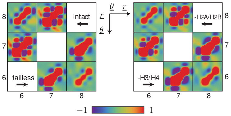
Color-coded representation of the rescaled global force constant matrices for the central three nucleosomes of 13-nucleosome chromatin constructs with intact or modified nucleosomes. The matrix on the left represents the force constants for intact nucleosomes versus tailless nucleosomes, while the matrix on the right represents the force constants for nucleosomes without H2A·H2B tails (-H2A/H2B) versus nucleosomes without H3·H4 tails (-H3/H4). The black mesh separates the block matrices corresponding to different pairs of nucleosomes. The axes and variables in the upper right corner denote the ordering of rigid-body parameters within each block matrix, and the color-scale at the bottom depicts the level of inverse covariance (i.e., the relative magnitude of the force constants).

We first notice that the force constants obtained for constructs with intact nucleosomes (upper triangle in the left half of Figure 5) resemble those reported in Figure 4 for longer constructs with 28-bp linkers. Moreover, the pattern of interactions associated with the intact nucleosomes resembles that obtained for constructs with nucleosomes missing H2A and H2B tails. We find different patterns for constructs made up of tailless nucleosomes or nucleosomes missing the tails of histones H3 and H4, and we see that these two constructs more closely resemble one another than the constructs with intact nucleosomes or without H2A and H2B tails. The removal of tail charges appears to lessen the interdependence, i.e., correlations, of rigid-body parameters, as evidenced by the color changes (corresponding to reductions in magnitude) of the off-diagonal entries in the force constant matrices. The removal of H3 and H4 tails appears to have a particularly significant effect on the coupling of the angular motions and displacements of successive nucleosomes and on the spatial arrangements of the second neighbors (i.e., (i, i + 2) pair). The changes in the force constant matrices underlie the large-scale deformations of the nucleosomal arrays that bring terminal residues in close proximity and subsequently allow for the interactions of attached transcriptional proteins.

3.5. Ideal polymer simulations

We use the results of our covariance analysis to build an ideal polymer model. The model takes the effective pair potentials obtained from the covariance analysis to describe the interactions of nucleosomes within chromatin. In other words, we now model chromatin as a collection of interacting nucleosomes, a great simplification of the system that makes it possible to simulate much longer fragments than with our base-pair-level mesoscale model. Once again, this higher-order approach is analogous to what has been previously done with DNA using a rigid base-pair model [30].

We consider a set of N_ncp nucleosomes and we denote p(i, j) the six rigid-body parameters describing the relative spatial arrangement of the ith and jth nucleosomes. The rest state for the nucleosome pair (i, j) is denoted $\underset{\_}{\overline{p}}(i,j)$ and the associated force constant matrix is denoted Q(i, j). We evaluate the total energy E of the chromatin fragment by computing the energy associated with each nucleosome pair, that is:

$$E=\frac{1}{2}\sum _{(i,j)/\mid i-j\mid \le n_{int}}\left[\frac{1}{2}{\left(\underset{\_}{p}(i,j)-\underset{\_}{\overline{p}}(i,j)\right)}^{\top }\mathit{Q}(i,j)(\underset{\_}{p}(i,j)-\underset{\_}{\overline{p}}(i,j))\right],$$ (5)

where the summation is restricted to the (i, j) pairs that are not sequentially farther apart than n_int nucleosomes. The outer factor of ½ in this expression avoids double counting pair interactions. The model only requires knowledge of the force constant matrices Q(i, j) and the vectors $\underset{\_}{\overline{p}}(i,j)$ describing the rest states of the various nucleosome pairs. The other parameter of the model, n_int, corresponds to the extent of nucleosome-nucleosome interactions. Here we choose n_int = 5; that is, we consider interactions between nucleosomes up to the (i, i + 5) pair.

The ideal polymer simulations are set up as regular MCMC simulations, in which at each step we select an (i, i+1) pair of nucleosomes and alter the corresponding rigid-body parameters by adding a randomly generated perturbation. The modified configuration is then accepted or rejected based on the Metropolis-Hasting algorithm [26,27].

We illustrate the method with chromatin constructs of 300 and 1000 nucleosomes with linker lengths of 21 bp or 24 bp. We show in Figure 6 selected snapshots of such constructs, and in Figure 7 we show the end-to-end distance distributions for construct with 300 nucleosomes. In addition, we fit the distributions in Figure 7 with the Gaussian-chain formula, that is:

$$P(r)=\frac{4\pi r^2}{{\left(\frac{2}{3}\pi \langle r^2\rangle \right)}^{3/2}}exp\left(-\frac{3r^2}{2\pi \langle r^2\rangle }\right).$$ (6)

Figure 6.

Snapshots of chromatin constructs generated with our ideal polymer simulations. The depicted constructs contain 300 and 1000 nucleosomes (ncps) with linker lengths of 21 bp or 24b p. The sequential color-coding (red-white) highlights the twofold periodicity found in the average constructs.

Figure 7.

End-to-end distance distributions and Gaussian-chain fits for chromatin constructs containing 300 nucleosomes with linker lengths equal to (blue) 21 bp and (red) 24 bp. The histograms represent the end-to-end distance distributions collected for the two types of constructs in our ideal polymer simulations. The solid lines denote the Gaussian-chain fits obtained with Equation (6). Note that, the distribution of the more flexible construct (21 bp, in blue) follows Gaussian chain statistics, whereas that of the more rigid construct (24 bp, in red) differs substantially from a Gaussian chain. The histogram data are based on 20,000 configurations generated in our ideal polymer simulations.

The results in Figure 7 reveal two different behaviors for constructs with 300 nucleosomes, depending on the linker length. The end-to-end distance for the chromatin construct with 21-bp linkers follows Gaussian-chain statistics, whereas there is a clear discrepancy between the predicted Gaussian-chain behavior and the distribution collected in our simulations for the construct with 24-bp linkers (compare the red solid line with the red histograms in Figure 7). Indeed, the distribution for the latter construct appears to be closer to those obtained with worm-like chain models (see the results in [32]). This suggests that the construct with 21-bp linkers is more flexible than that with 24-bp linkers. We show below two different approaches to characterize the persistence lengths of these constructs and confirm the greater flexibility of the construct with shorter linkers.

We evaluate the persistence length by first computing the tangent correlations along the construct and then fitting the data with a ribbon-like model [33] (see Appendix B). We find persistence lengths of ~ 28 ncp and ~ 55 ncp for chromatin constructs with linker lengths of 21 bp and 24 bp, respectively, where the lengths are expressed in units of nucleosomes rather than through-space distances (see below). These persistence lengths correspond to respective genomic distances of ~ 4.7 kbp and ~ 9.4 kbp, a remarkable change in chain flexibility for a very small variation in the linker length.

Note that, we choose not to express these persistence lengths in a distance unit as the values do not necessarily reflect the physical length over which the tangent correlations vanish. Indeed, the computed values strongly depend on fiber conformation (i.e., the suprahelical arrangement of nucleosomes). In other words, because the folding of chromatin into a fiber-like structure is highly sensitive to the spacing between nucleosomes (i.e., the DNA linker length) it is difficult to define a physically relevant contour length. In particular, this raises the question of how to use polymer models that involve a precise definition of the contour length. We are currently investigating how to define coarse-grained centerlines for chromatin constructs with very different helical arrangements.

In order to obtain additional measurements of the persistence length for the same systems, we extracted persistence vectors along the constructs (i.e., configurational averages of the chain vectors connecting each nucleosome to the first nucleosome, expressed in the reference frame of the first nucleosome) [4] (see Appendix B). The variation of the vectorial components along the two chains shows the asymptotic behavior expected when parts of the chain are no longer directionally correlated (Figure 8). We determine the persistence lengths from the norm of the limiting persistence vectors, obtaining values of ~ 76.9 nm for the construct with 21-bp linkers and ~ 149.4 nm for the construct with 24-bp linkers. Interestingly, two of the components ( $a_y^{21}$ and $a_z^{21}$) of the persistence vector of the construct with 21-bp linkers converge to significantly large values (~ 35 nm and ~ 68 nm, respectively). By contrast, a single component ( $a_y^{24}$) captures most of the magnitude of the persistence vector for the construct with 24-bp linkers. Importantly, the ratio of persistence lengths is very similar to the ratio of the persistence lengths obtained by fitting the tangent correlations.

Figure 8.

Components of the persistence vector along chromatin construct with 300 nucleosomes for linker lengths equal to (thick lines) 21 bp and (thin lines) 24 bp. The color-coding denotes the three components of the persistence vectors.

The components of the persistence vector reveal other useful information about the chromatin constructs. Specifically, the limiting magnitudes of the three components provide insights into the orientation of the nucleosomes with respect to the fiber axis. For example, in the case of the construct with linker lengths of 24 bp, the largest component of the limiting persistence vector lies along the y axis (denoted $a_y^{24}$ in Figure 8). This is the component of the vector parallel to the y axis of the local frame attached to the first nucleosome of the construct (see Figure 1 for the local frame axes). Examination of representative chain configurations shows that this direction corresponds to the direction of the local suprahelical axis around which the nucleosomes are organized (see the zoom-in inset in the top right of Figure 6, where the y-axes run across the more open sides of the nucleosome wedges, in the same direction as the lightly shaded lines seen on specific wedges). The same interpretation holds for the 21-bp linker construct, for which the two main components lie along the y– and z–axes. As evident from the zoom-in inset in the top left of Figure 6, the nucleosomes are organized such that both the normals and the axes across the open sides of the wedges describe comparable angles with respect to the fiber axis. This particular direction corresponds, within the local frame of the first nucleosome, to a vector with components of comparable magnitude along the y– and z–axes (see the definition of the local frame in Figure 1). The periodicity in smaller components of the persistence length over short lengths provides additional insights into the geometry of the simulated fibers, as will be described elsewhere.

4. Discussion

The mesoscale model of nucleosomal arrays presented in this work makes it possible to investigate how nucleosome positioning, at the level of a single base pair, (i.e., linker length) influences the overall architecture and deformations of chromatin. The model also allows us to account for chemical modifications of nucleosomes, such as histone-tail modifications, by removing the relevant charges in the system. We implemented the model in a methodical study of short chromatin constructs containing up to twenty nucleosomes with linker lengths ranging from 15 bp to 80 bp. We have extracted, from these simulations, two global quantities characterizing the stiffness and the magnitude of the interactions in the constructs. These data reveal a remarkable effect of nucleosome positioning on chromatin properties. For linker lengths above 30 bp, we find a clear distinction between constructs with linker lengths corresponding to integral numbers of DNA helical repeats and those with linker lengths equal to half-integral numbers of repeats. The former have a lower effective stiffness and a higher interaction score per nucleosome. For constructs with linker lengths shorter than 30 bp, excluded-volume effects and the very short distances between nucleosomes appear to have a significant impact on chromatin properties. In addition, we have introduces a method to derive effective ‘local’ nucleosome pairwise potentials from the mesoscale simulations. This information makes it possible to perform simulations of regularly repeating chromatin constructs over a much larger scale (i.e., ideal polymer simulations) than the mesoscale calculation and, therefore, to estimate the persistence lengths of long chromatin fibers. To illustrate the approach we focus on two constructs with different, but close, linker lengths and estimate the associated persistence lengths.

The ideal polymer simulations show that the statistical properties of the long chromatin constructs strongly depend on nucleosome positioning. The distributions of end-to-end distances can differ appreciably, even for a small change in linker length. For example, for constructs of 300 nucleosomes we find that a change of 3 bp in linker length is enough to shift the end-to-end distribution from Gaussian to worm-like chain behavior. Moreover, our estimates of the persistence lengths for these two constructs show a two-fold increase over the 3-bp change in linker length. Our findings therefore bring into question the applicability of simple polymer models, such as worm-like and Gaussian chain models, in the interpretation of certain chromatin experiments. Our computations suggest that the length of the chromatin chain and the precise locations of nucleosomes along the construct can drive the statistical properties of the system towards very different behaviors ranging from stiff to floppy polymers. As a consequence, without minimal a priori knowledge of these molecular features, the choice of one polymer model versus another to fit experimental or numerical data could bias the derivation of quantities such as the persistence length.

We also present two different methods to estimate the persistence lengths of the chromatin constructs generated in the ideal polymer simulations. The first method is based on a worm-like chain model that takes account of the superhelical arrangement of nucleosomes and is referred to as a ribbon-like model [33]. The second method relies on the computation of the persistence vector along the construct [4]. The two methods yield different results in different units, although the relative magnitudes of the values obtained for two different constructs are very close. Notably, our estimates of the persistence length for chromatin constructs with linker lengths equal to 21 bp and 24 bp (76.9 nm and 149.4 nm, respectively) fall in the range of previously reported values. We remark, however, that, it is complicated to define the persistence length of a chromatin construct in a unique way. For example, the persistence lengths obtained from the ribbon-like model assume worm-like chain behavior of the chromatin chain, which, as mentioned above, is not necessarily the case. Thus, the persistence vector approach might provide a more unbiased estimate of the persistence length, as well as information about the local geometry of the chromatin fiber.

The characterization of chromatin stiffness is a difficult task because of the structural plasticity of the long, protein-DNA assembly. From this perspective, unraveling the relationship between chromatin architecture and nucleosome positioning is an important task. In this study we have focused on regularly repeating chromatin constructs, that is, arrays of nucleosomes regularly positioned along DNA. An exciting, and more biologically relevant, development of our work, will be to focus on chromatin constructs with the more irregularly spaced nucleosomes detect in vivo, e.g., [34].

Appendix A. Geometry of a collection of nucleosomes

We present here the geometrical method used to describe a collection of nucleosomes in terms of rigid-body parameters. Each nucleosome is represented by an orthonormal frame, and the set of all such frames is used to characterize the geometry of all pairs of nucleosomes within the chromatin system.

For two nucleosome frames centered respectively at positions x₁ and x₂, we denote d₁ and d₂ the matrices containing the nucleosome frame axes as columns. The relative arrangement of a pair of nucleosomes is then described by six rigid-body parameters: three angles describing the rotation between the two frames and three components describing the displacement vector.

The three angles, denoted θ₁, θ₂, θ₃, are defined in the exact same way as the tilt, roll, and twist angles introduced for the description of DNA base-pair step geometry (see references [21,22] for more details). That is, these angles are obtained from the rotation matrix d₁^⊤d₂. The three translational parameters, denoted r = (r₁, r₂, r₃) ^⊤ correspond to the projection of the joining vector x₂ − x₁ on the frame of the first nucleosome, that is, r = d₁^⊤(x₂ − x₁). The six parameters form a vector denoted p(1, 2) for nucleosomes 1 and 2.

For a collection of nucleosomes on an arbitrary chromatin chain, one can compute the rigid-body parameters associated with each pair of nucleosomes, and then for a set of such chains determine the mean values and standard deviations of the parameters. While the computation is straightforward for translational parameters, the angular parameters follow circular statistics and one needs to take account of their periodicity. For a series of angular values {α_i} we define the mean value 〈α〉, following [35], as:

$$tan\langle \alpha \rangle =\frac{\langle sin\alpha \rangle }{\langle cos\alpha \rangle }=\frac{{\sum }_{i=1}^{N}sin{\alpha }_i}{{\sum }_{i=1}^{N}cos{\alpha }_i},$$ (A.1)

where N is the number of values. We also account for the angular periodicity when computing differences between two angles. For two angle α₁ and α₂ we define Δα = α₁ − α₂ as:

$$\mathrm{\Delta }\alpha =\text{sign}\left(\left(\begin{array}{c}cos{\alpha }_1\hfill \\ sin{\alpha }_1\hfill \\ 0\end{array}\right)\times \left(\begin{array}{c}cos{\alpha }_2\hfill \\ sin{\alpha }_2\hfill \\ 0\end{array}\right)·\left(\begin{array}{c}0\\ 0\\ 1\end{array}\right)\right)arccos\left(\left(\begin{array}{c}cos{\alpha }_1\hfill \\ sin{\alpha }_1\hfill \\ 0\end{array}\right)·\left(\begin{array}{c}cos{\alpha }_2\hfill \\ sin{\alpha }_2\hfill \\ 0\end{array}\right)\right).$$ (A.2)

With the help of these formulas we can efficiently compute angular means and standard deviations across a set of parameters.

Appendix B. Persistence length and persistence vector

For a given type of construct, we extract from our ideal polymer simulations the origins of every nucleosomes, denoted {xⁱ}. We use those data to extract the persistence length of the simulated constructs using two different approaches.

Figure B1.

Tangent correlations along a chromatin construct of 300 nucleosomes separated by linkers of 24 bp. The blue line denotes the fit obtained with Equation (B.1). The inset represents a zoom on the first 40 nucleosomes; in this plot the red dots represent the tangent correlations extracted from our ideal polymer simulations. Note that, the oscillations in the tangent correlations are typical of a superhelical arrangement.

First, we rely on a ribbon model [33], which, like the worm-like chain model, defines the persistence length as the typical length over which the correlations in the tangent decrease by a factor 1/e. In other words, we compute the tangent correlations along the construct, that is, the discrete function 〈t₁ · t_i〉, where t_i = xⁱ⁺¹ − xⁱ/|xⁱ⁺¹ − xⁱ|. Our numerical results are then fitted using the following formula [33]:

$$\langle {\underset{\_}{t}}_1·{\underset{\_}{t}}_i\rangle =e^{-\frac{i}{L^{\mathrm{R}}}}cos(ki),$$ (B.1)

where L^R is the persistence length in units of number of nucleosomes and k is related to the helical periodicity of the chromatin construct. We show in Figure B1 an example of such a fit for a chromatin construct containing 300 nucleosomes with linker lengths equal to 24 bp. The oscillations in the tangent correlations are a consequence of the suprahelical arrangement of nucleosomes within the construct.

In addition, we also compute the persistence length with the approach of Flory [4], that is, we compute the components of the persistence vector a(i) along the system as:

$$\underset{\_}{a}(i)={\mathit{d}}^1\langle {\underset{\_}{x}}^i-{\underset{\_}{x}}^1\rangle ,$$ (B.2)

where d¹ is the local frame of the first nucleosome, which is left unchanged during all the simulations. The components of the vector a(i) are expected to reach a plateau after a certain number of nucleosomes. Those asymptotic values contain information about the geometry of the system as well as about the persistence length.

References

- 1.Schoenfelder S, Clay I, Fraser P. Curr Opin Genet Dev. 2010;20:127–133. doi: 10.1016/j.gde.2010.02.002. [DOI] [PubMed] [Google Scholar]
- 2.Olson WK, Marky NL, Jernigan RL, Zhurkin VB. J Mol Biol. 1993;232:530–554. doi: 10.1006/jmbi.1993.1409. [DOI] [PubMed] [Google Scholar]
- 3.Kratky O, Porod G. Rec Trav Chim Pays-Bas. 1949;68:1106–1122. [Google Scholar]
- 4.Flory PJ. Proc Natl Acad Sci, USA. 1973;70:1819–1823. doi: 10.1073/pnas.70.6.1819. [DOI] [PMC free article] [PubMed] [Google Scholar]
- 5.Bystricky K, Heun P, Gehlen L, Langowski J, Gasser SM. Proc Natl Acad Sci, USA. 2004;101:16495–16500. doi: 10.1073/pnas.0402766101. [DOI] [PMC free article] [PubMed] [Google Scholar]
- 6.Dekker J. J Biol Chem. 2008;283:34532–34540. doi: 10.1074/jbc.M806479200. [DOI] [PMC free article] [PubMed] [Google Scholar]
- 7.Tjong H, Gong K, Chen L, Alber F. Genome Res. 2012;22:1295–1305. doi: 10.1101/gr.129437.111. [DOI] [PMC free article] [PubMed] [Google Scholar]
- 8.Cui Y, Bustamante C. Proc Natl Acad Sci, USA. 2000;97:127–132. doi: 10.1073/pnas.97.1.127. [DOI] [PMC free article] [PubMed] [Google Scholar]
- 9.Bancaud A, Conde e Silva N, Barbi M, Wagner G, Allemand JF, Mozziconacci J, Lavelle C, Croquette V, Victor JM, Prunell A, Viovy JL. Nature Str Mol Biol. 2006;13:444–450. doi: 10.1038/nsmb1087. [DOI] [PubMed] [Google Scholar]
- 10.Celedon A, Nodelman IM, Wildt B, Dewan R, Searson P, Wirtz D, Bowman GD, Sun SX. Nano Lett. 2009;9:1720–1725. doi: 10.1021/nl900631w. [DOI] [PMC free article] [PubMed] [Google Scholar]
- 11.Kruithof M, Chien FT, Routh A, Logie C, Rhodes D, van Noort J. Nature Str Mol Biol. 2009;16:534–540. doi: 10.1038/nsmb.1590. [DOI] [PubMed] [Google Scholar]
- 12.Hajjoul H, Mathon J, Ranchon H, Goiffon I, Mozziconacci J, Albert B, Carrivain P, Victor JM, Gadal O, Bystricky K, Bancaud A. Genome Res. 2014;23:1829–1838. doi: 10.1101/gr.157008.113. [DOI] [PMC free article] [PubMed] [Google Scholar]
- 13.Schiessel H, Gelbart WM, Bruinsma R. Biophys J. 2001;80:1940–1956. doi: 10.1016/S0006-3495(01)76164-4. [DOI] [PMC free article] [PubMed] [Google Scholar]
- 14.Ben-Haïm E, Lesne A, Victor JM. Phys Rev E Stat Nonlin Soft Matter Phys. 2001;64:051921. doi: 10.1103/PhysRevE.64.051921. [DOI] [PubMed] [Google Scholar]
- 15.Wedemann G, Langowski J. Biophys J. 2002;82:2847–2859. doi: 10.1016/S0006-3495(02)75627-0. [DOI] [PMC free article] [PubMed] [Google Scholar]
- 16.Rubtsov M, Polikanov Y, Bondarenko V, Wang YH, Studitsky VM. Proc Natl Acad Sci, USA. 2006;102:17690–17695. doi: 10.1073/pnas.0603819103. [DOI] [PMC free article] [PubMed] [Google Scholar]
- 17.Kulaeva OI, Zheng G, Polikanov YS, Colasanti AV, Clauvelin N, Mukhopadhyay S, Sengupta AM, Studitsky VM, Olson WK. J Biol Chem. 2012;287:20248–20257. doi: 10.1074/jbc.M111.333104. [DOI] [PMC free article] [PubMed] [Google Scholar]
- 18.Nizovtseva EV, Polikanov YS, Kulaeva OI, Clauvelin N, Postnikov Y, Dimitrov S, Bustin M, Olson WK, Studitsky VM. 2014 doi: 10.1134/S0026898419060132. submitted. [DOI] [PMC free article] [PubMed] [Google Scholar]
- 19.Olson WK, Clauvelin N, Colasanti AV, Singh G, Zheng G. Biophys Rev. 2012;4:171–178. doi: 10.1007/s12551-012-0093-8. [DOI] [PMC free article] [PubMed] [Google Scholar]
- 20.Arya G, Schlick T. Proc Natl Acad Sci, USA. 2006;103:16236–16241. doi: 10.1073/pnas.0604817103. [DOI] [PMC free article] [PubMed] [Google Scholar]
- 21.Coleman BD, Olson WK, Swigon D. J Chem Phys. 2003;118:7127–7140. [Google Scholar]
- 22.Dickerson RE, Bansal M, Calladine CR, Diekmann S, Hunter WN, Kennard O, von Kitzing E, Lavery R, Nelson HCM, Olson WK, Saenger W, Shakked Z, Sklenar H, Soumpasis DM, Tung CS, Wang AHJ, Zhurkin VB. Nucleic Acids Res. 1989;17:1797–1803. [Google Scholar]
- 23.Luger K, Mader AW, Richmond RK, Sargent DF, Richmond TJ. Nature. 1997;389:251–260. doi: 10.1038/38444. [DOI] [PubMed] [Google Scholar]
- 24.Potoyan DA, Papoian GA. J Am Chem Soc. 2011;133:7405–7415. doi: 10.1021/ja1111964. [DOI] [PubMed] [Google Scholar]
- 25.Manning GS. Quart Rev Biophys. 1978;11:179–246. doi: 10.1017/s0033583500002031. [DOI] [PubMed] [Google Scholar]
- 26.Metropolis N, Rosenbluth AW, Rosenbluth MN, Teller AH, Teller E. J Chem Phys. 1953;21:1087–1092. [Google Scholar]
- 27.Hastings WK. Biometrika. 1970;57:97–109. [Google Scholar]
- 28.Smith R. 2001–2014 http://www.ode.org.
- 29.Liu JS. Monte Carlo Strategies in Scientific Computing. New York: Springer-Verlag; 2001. [Google Scholar]
- 30.Olson WK, Gorin AA, Lu XJ, Hock LM, Zhurkin VB. Proc Natl Acad Sci, USA. 1998;95:11163–11168. doi: 10.1073/pnas.95.19.11163. [DOI] [PMC free article] [PubMed] [Google Scholar]
- 31.Gonzalez O, Petkevičiūė D, Maddocks JH. J Chem Phys. 2013;138:055102. doi: 10.1063/1.4789411. [DOI] [PubMed] [Google Scholar]
- 32.Becker N, Rosa A, Everaers R. Euro Phys J E. 2010;32:53–69. doi: 10.1140/epje/i2010-10596-0. [DOI] [PubMed] [Google Scholar]
- 33.Giomi L, Mahadevan L. Phys Rev Lett. 2010:238104. doi: 10.1103/PhysRevLett.104.238104. [DOI] [PubMed] [Google Scholar]
- 34.Brogaard K, Xi L, Wang JP, Widom J. Nature. 2012;486:496–501. doi: 10.1038/nature11142. [DOI] [PMC free article] [PubMed] [Google Scholar]
- 35.Fisher NI. Statistical Analysis of Circular Data. Cambridge: Cambridge University Press; 1993. [Google Scholar]