High-resolution mapping of the protein interaction network for the human transcription machinery and affinity purification of RNA polymerase II-associated complexes

Abstract

Thirty years of research on gene transcription has uncovered a myriad of factors that regulate, directly or indirectly, the activity of RNA polymerase II (RNAPII) during mRNA synthesis. Yet many regulatory factors remain to be discovered. Using protein affinity purification coupled to mass spectrometry (AP-MS), we recently unraveled a high-density interaction network formed by RNAPII and its accessory factors from the soluble fraction of human cell extracts. Validation of the dataset using a machine learning approach trained to minimize the rate of false positives and false negatives yielded a high-confidence dataset and uncovered novel interactors that regulate the RNAPII transcription machinery, including a new protein assembly we named the RNAPII-Associated Protein 3 (RPAP3) complex.

1. Introduction

Protein affinity purification coupled to mass spectrometry (AP-MS) is a method of choice for the characterization of protein complexes and the identification of protein interaction partners. Among the various possible strategies for conducting AP-MS, the use of an affinity tag attached to the protein of interest has been widely used. For example, the Tandem Affinity Purification (TAP) procedure was used by many different groups in yeast and mammalian cells to characterize protein interaction networks and complexes involved in various cellular processes [1,2]. The output of the AP-MS procedure is usually a list of proteins in which each putative interactor is attributed a mass spectrometry (MS) score through the use of specialized software such as MASCOT or SEQUEST. Making sense of these lists is often the major challenge of the procedure. Even if a negative control is used to identify proteins that contaminate the affinity purified eluate (e.g. proteins found both in the control and affinity purified eluates), the challenge remains significant, especially when dealing with interactors that are either unexpected (proteins known to function in a different pathway or process) or that have not been previously characterized and have not been assigned a function. However, these proteins that are unexpected in a list of candidate interactors are often the most promising in terms of proteomic discovery.

As the experimental validation of the complete list of putative interaction partners (preys) for a tagged protein (bait) is not an option because it may contain many proteins, more manageable solutions need to be defined. Five specific solutions are most convenient. First, the use of additional purification steps that would “clean” the affinity purified eluate from contaminating proteins have been used in many reports [3]; one caveat of this solution is that weak, transient interactions will more readily be disrupted, leading to the loss of putatively interesting interactors. Secondly, the use of high-accuracy mass spectrometers leads to a significant decrease in the rate of false positives generated by the inaccuracy in the molecular mass of peptides used in protein identification. Thirdly, the use of expression systems that avoid the overexpression of the tagged proteins has been shown to minimize the occurrence of spurious interactions in protein–protein interaction datasets. Fourthly, the development of computational procedures that help to increase the confidence in protein–protein interaction datasets is often powerful and very useful [4]. Finally, a number of approaches could be employed, ranging from label-free methods to more accurate strategy such as SILAC, to perform quantitative MS comparison of negative controls and AP samples. Quantitative MS is a highly valuable strategy to differentiate real interacting proteins from co-purified species.

In previous work, we reported the development and use of a multistep procedure for the systematic analysis of the protein interaction network for the human RNAPII transcription machinery [5,6]. This proteomic procedure couples (i) affinity purification of tagged proteins (TAP-tagging) from the soluble cell fraction in gentle conditions in order to preserve weak, transient interactions, (ii) the identification of co-purified proteins using sensitive, high-accuracy mass spectrometry, (iii) the validation of protein–protein interactions using a computational algorithm trained to minimize the rate of false positive and false negative interactions and (iv) the schematic representation of protein–protein interaction networks to visualize protein connectivity. A key aspect of our procedure relies on the reciprocal tagging of preys identified in our experiments. This step is important to confirm some interactions and to expand the dataset. In this procedure, the accuracy of the network that we end up mapping increases proportionally with the number of baits used in our AP-MS experiments. As compared to the dataset we published in 2007 [6], which was built using 32 baits, the dataset used in the current report uses 77 baits. Coupled to other technical improvements of the procedure, especially regarding MS accuracy and sensitivity, the dataset used in the current report permits a higher resolution in mapping the human RNAPII transcription network. A schematic representation of our procedure is presented in Fig. 1.

Fig. 1.

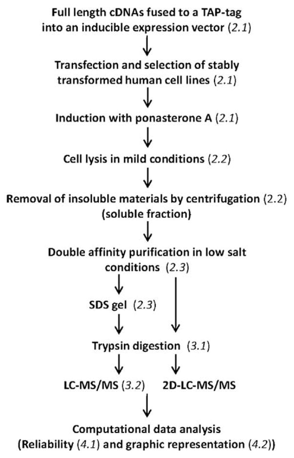
Schematic representation of our multi-step proteomics procedure. The procedure couples the regulated expression of affinity tagged proteins (baits) in human cells, the purification of putative interaction partners (preys) in the form of protein complexes, the identification of co-purified proteins using mass spectrometry (MS) and the computational validation and analysis of the data. Each step is referred to the appropriate section in the text.

Our previous 32-bait dataset allowed the identification of two novel factors that regulate the activity of the positive transcription elongation factor P-TEFb, a factor that is recruited to the RNAPII elongation complex where it functions by phosphorylating the RNAPII CTD and negative elongation factors such as NELF and DSIF to stimulate transcriptional elongation. The newly identified factors favor the sequestration of P-TEFb away from chromatin DNA. Indeed, the methylphosphate capping enzyme MEPCE and the RNA-binding protein LARP7 associate with and stabilize the 7SK snRNA which, in association with inhibitory proteins termed HEXIMs, binds to P-TEFb and prevents its recruitment to transcribing RNAPII complexes [6,7]. The formation of transcriptionally active P-TEFb requires its dissociation from the HEXIM-7SK inhibitory complex.

The 32-bait dataset also identified a set of proteins that are tightly connected to RNAPII [5,6]. Accordingly, these proteins were named RNAPII-Associated Proteins (RPAPs). Although the exact function of these factors remains elusive, the 77-bait dataset now reveals that one of these RPAPs, RPAP3, is part of an 11-subunit protein complex akin to that described by Gstaiger and colleagues [8] (see figures for details). Of note, and in contrast to the aforementioned report, we have not found STAP1 in any of our purifications, and our complex is more similar in composition with that described in a recent report [9], with the exception that, unlike POLR2E (RPB5), our data do not support the idea that the RNAPIII subunit POLR3A (RPC1) is a bona fide component of this complex. In addition to POLR2E, this complex contains human homologs of the yeast R2TP complex [10,11], including RPAP3 (Tah1, Spag), PIH1D1 (Pih1, Nop17), RUVBL1 (Tip49) and RUVBL2 (Tip48). WDR92 (Monad), whose interaction with RPAP3 was recently published [12], is also present but unlike R2TP, this complex comprises PFDN2 and PFDN6 (HKE2), two subunits shared with the canonical prefoldin complex, and three prefoldin-like proteins, UXT (ART-27), PDRG1 and C19orf2 (URI, RMP). The latter is a well-characterized protein known to bind POLR2E [13] and has a conserved role in TOR signaling [8,14]. Other proteins co-purified with some tagged subunits of the RPAP3 (R2TP/Prefoldin-like) complex, notably POLR2A (RPB1), RPAP2, RPAP4 and RP11-529I10.4 (DPCD), confirming that these are likely transient interactors, but not components of the stable complex. The unidirectionality of these interactions also supports this conclusion.

2. Affinity purification of RNA polymerase II and its associated proteins

2.1. Generation of stable human cell lines expressing TAP-tagged proteins

Full-length human cDNAs (Open Biosystems) were amplified by PCR and cloned into the pMZI vector using either XhoI, XbaI, SalI, NotI or NdeI sites. pMZI drives the expression of proteins with a C-terminal TAP-tag in mammalian cells under the control of an ecdysone inducible promoter [1]. The resulting plasmids were transfected into HEK 293 cells (ATCC) previously transfected with pVgRxR (Invitrogen), which encodes the ecdysone receptor heterodimer. Stable clones were selected and grown in DMEM media supplemented by 10% fetal bovine serum, 2 mM glutamine, 30 μg/ml Bleocin (Calbiochem) and 300 μg/ml G418 (Invitrogen). Once the culture reached a volume of about one-hundred 150 mm plates and a confluency of 20%, the cells were induced in half of these plates in 3 μM ponasterone A (Invitrogen). The other half is maintained as is to serve as a negative control. Two days following induction, the cells were harvested in ice-cold PBS by tapping plates and centrifuged at 3000 rpm for 10 min at 4 °C in a SLA-3000 rotor (Sorvall). Supernatant was discarded and pellets (2.5–3 g of cells for each induced and non-induced cultures) were dislodged with 20 ml ice-cold PBS, transferred to 50 ml Falcon tubes and spun once more for 10 min at 4 °C in a table top centrifuge at 3000 rpm. Following decantation, the pellets were usually frozen at −70 °C before proceeding the next day with extraction of protein complexes.

2.2. Preparation of whole cell extracts

All of the following steps were performed on ice to limit protein precipitation and proteolysis. Buffer A (10 mM Hepes, pH 7.9, 1.5 mM MgCl₂, 10 mM KCl, 0.5 mM DTT, 0.5 mM AEBSF, complete EDTA-free protease inhibitor cocktail (Roche)) was added to the pellet with a ratio of 4/3 (ml/g of cells). The mixture was transferred to a 10 or 30 ml glass homogenizer (Wheaton) and the pellet was broken up by 10 gentle strokes while being careful not to create foam in the sample. By pipetting up and down, buffer B (50 mM Hepes, pH 7.9, 1.5 mM MgCl₂, 0.5 mM DTT, 0.5 mM AEBSF, 1.26 M K acetate, glycerol 75%) was mixed in the lysate with a ratio of 1/1 (ml/g of cells). Membranes were further disrupted by 10 extra pestle strokes. The lysate was poured into an ultracentrifuge tube and incubated for 30 min at 4 °C on a mixer and then spun at 37,000 rpm for 3 h at 4 °C in a 50.2TI rotor (Beckman Coulter). The soluble fraction was separated from insoluble materials and dialyzed overnight using 18 mm Spectra/Por 3 membranes (Spectrum Laboratories) in 3 l dialysis buffer (10 mM Hepes, pH 7.9, 0.1 mM EDTA, 0.1 mM DTT, 0.1 M K acetate, 10% glycerol). The following day, the cell extracts were transferred to 15 ml Corex tubes and centrifuged once more at 14,000 rpm for 30 min at 4 °C in a SS-34 rotor (Sorvall). The final protein concentration in the lysate is typically around 4 mg/ml.

2.3. Tandem-affinity purification

For each gram of cells harvested, 50 μl of the IgG sepharose 6 Fast Flow beads (GE Healtcare) used in the first affinity purification were washed by centrifugation at 3000g for 2 min at 4 °C once in 1 ml of Tris-saline Tween-20 (TST) buffer (50 mM Tris–HCl, pH 7.6, 150 mM NaCl, 0.05% Tween-20) and then twice in 500 μl immunoprecipitation (IPP) buffer (10 mM Tris–HCl, pH 8, 100 mM NaCl, 0.1% Triton X-100, 10% glycerol). The whole cell extract was incubated with the washed beads for 1 h at 4 °C on a mixer. The resin was then washed twice in 500 μl IPP before loading onto a Bio-spin disposable chromatography column (Bio-Rad). Five hundred microliter of TEV buffer (10 mM Tris–HCl, pH 8, 100 mM NaCl, 0.1% Triton X-100, 0.5 mM EDTA, 10% glycerol, 1 mM DTT) were allowed to drip out by gravity before plugging the column and adding 30 units of AcTEV protease (Invitrogen) in 200 μl of TEV. The column was incubated over night at 4 °C on a mixer to allow cleavage of the protein A component of the tagged polypeptide, thereby freeing the protein complexes from the IgG beads.

The next morning, the column was opened and drained into a tube containing 50 μl of calmodulin sepharose 4B beads (GE Healthcare) that were previously washed twice in 500 μl calmodulin binding (CBB) buffer (10 mM Tris–HCl, pH 8, 100 mM NaCl, 1 mM immidazole, 1 mM Mg acetate, 2 mM CaCl₂, 0.1% Triton X-100, 10% glycerol, 10 mM β-mercaptoethanol). The column was further washed with 50 μl of TEV and 2 × 300 μl of CBB all of which were eluted by gravity flow onto the calmodulin resin before adding 0.8 μl of 1 M CaCl₂ directly to the tube. The resulting mixture was incubated 2 h at 4 °C on a mixer. Following incubation, the beads were washed twice in 500 μl CBB and loaded into another Bio-spin column. To push out remaining CBB from the beads, 40 μl of calmodulin elution (CEB) buffer (10 mM Tris–HCl, pH 8, 100 mM NaCl, 1 mM immidazole, 1 mM Mg acetate, 2 mM EGTA, 10% glycerol, 10 mM β-mercaptoethanol) was added to the column. The protein complexes were then eluted from the beads by addition of two volumes of 100 μl and 150 μl of CEB. The eluate was frozen in liquid nitrogen and its volume was reduced to about 30 μl using a speed vac. The complexes were then separated on a 1 mm NuPAGE 4–12% Bis-Tris Gel (Invitrogen) followed by silver staining (see Fig. 2 for an example). Although yields and recoveries of protein complexes usually vary from bait to bait, probably because the accessibility of the affinity tag also varies depending on the bait, this procedure generally yields sufficient amounts of proteins to proceed successfully with mass spectrometry analysis.

Fig. 2.

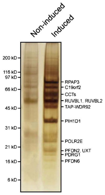
Purification of the TAP-tagged human RPAP3 complex. TAP eluates of induced or non-induced HEK 293 cells expressing TAP-tagged RPAP3 (WDR92) were analyzed by SDS–PAGE. Gel lanes were cut from top to bottom, singling out discernable proteins, slices were digested with trypsin, and analyzed by LC-MS/MS. The position of molecular weight markers (left) and that of identified components of the RPAP3 and CCT complexes (right) are shown.

3. Analysis of protein complexes using mass spectrometry

3.1. Protein digestion with trypsin

The in-gel digestion protocol is based on the results obtained by Havlis et al. [15]. This protocol allows performing the protein digestion step in 6 h without compromising the peptide yield over conventional trypsin digestion protocols (data not shown). The entire gel lane was excised into 18–20 bands and each band was cut in 1 mm³ pieces. For the following steps, all volumes were adjusted according to the volume of gel pieces. Gel pieces were first washed with water for 5 min and destained twice with the destaining buffer (100 mM sodium thiosulfate, 30 mM potassium ferricyanide) for 15 min. An extra wash of 5 min was performed after destaining with a buffer of ammonium bicarbonate (50 mM). Gel pieces were then dehydrated with acetonitrile. Proteins were reduced by adding the reduction buffer (10 mM DTT, 100 mM ammonium bicarbonate) for 30 min at 40 °C, and then alkylated by adding the alkylation buffer (55 mM iodoacetamide, 100 mM ammonium bicarbonate) for 20 min at 40 °C. Gel pieces were dehydrated and washed at 40 °C by adding ACN for 5 min before discarding all the reagents. Gel pieces were dried for 5 min at 40 °C and then re-hydrated at 4 °C for 40 min with the trypsin solution (6 ng/μl of trypsin sequencing grade from Promega, 25 mM ammonium bicarbonate). The concentration of trypsin was kept low to reduce signal suppression effects and background originating from autolysis products when performing LC-MS/MS analysis. Protein digestion was performed at 58 °C for 1 h and stopped with 15 μl of 1% formic acid/2% acetonitrile. Supernatant was transferred into a 96-well plate and peptides extraction was performed with two 30-min extraction steps at room temperature using the extraction buffer (1% formic acid/50% ACN). All peptide extracts were pooled into the 96-well plate and then completely dried in vacuum centrifuge. The plate was sealed and stored at −20 °C until LC-MS/MS analysis.

3.2. LC-MS/MS

Prior to LC-MS/MS, peptide extracts were re-solubilized under agitation for 15 min in 12 μl of 0.2% formic acid and then centrifuged at 2000 rpm for 1 min. The LC column was a C18 reversed-phase column packed with a high-pressure packing cell. A 75 μm i.d. fused silica capillary of 100 mm long was packed with the C18 Jupiter 5 μm 300 Å reverse-phase material (Phenomenex). This column was installed on the nanoLC-2D system (Eksigent) and coupled to the LTQ Orbitrap (ThermoFisher Scientific). The buffers used for chromatography were 0.2% formic acid (buffer A) and 100% acetonitrile/0.2% formic acid (buffer B). During the first 12 min, 5 μl of sample were loaded on column with a flow of 650 nl/min and, subsequently, the gradient went from 2–80% buffer B in 20 min and then came back to 2% buffer B for 10 min. LC-MS/MS data acquisition was accomplished using a four scan event cycle comprised of a full scan MS for scan event 1 acquired in the Orbitrap which enables high resolution/high mass accuracy analysis. The mass resolution for MS was set to 30,000 (at m/z 400) and used to trigger the three additional MS/MS events acquired in parallel in the linear ion trap for the top three most intense ions. Mass over charge ratio range was from 380 to 2000 for MS scanning with a target value of 500,000 charges and from ~1/3 of parent m/z ratio to 2000 for MS/MS scanning with a target value of 20,000 charges. The data dependent scan events used a maximum ion fill time of 100 ms and 1 microscan to increase the duty cycle for ion detection. Target ions already selected for MS/MS were dynamically excluded for 15 s. Nanospray, capillary and tube lens voltages were set to 0.9–1.6 kV, 5 and 100 V, respectively. Capillary temperature was set to 200 °C. MS/MS conditions were: normalized collision energy, 35 V; activation q, 0.25; activation time, 30 ms.

In some experiments, we used two-dimensional (2D-) LC-MS/MS on peptide mixtures generated by trypsin digestion of TAP eluates that have not been submitted to SDS gel analysis. In most cases, the gel-free 2D-LC-MS/MS method produced results that were mainly confirmatory (and in some cases complementary) to the gel-based method described in the previous paragraph. For this reason 2D-LC-MS/MS will not be described in details here.

3.3. Protein identification

Protein database searching was performed with Mascot 2.1 (Matrix Science) against the human NCBInr protein database. The mass tolerances for precursor and fragment ions were set to 10 ppm and 0.6 Da, respectively. Trypsin was used as the enzyme allowing for up to 2 missed cleavages. Carbamidomethyl and oxidation of methionine were allowed as variable modifications.

4. MS data analysis

4.1. Reliability of protein–protein interactions

The list of candidate prey proteins identified by MS for a given bait is likely to contain a certain fraction of false-positives. These erroneous interactions could be the result of incorrect peptide identification, transient/indirect interactions, contamination of gel lanes, etc. The rate of incorrect peptide identification can be estimated using a decoy database [16], consisting for example of reversed protein sequences. The number of peptide matches to the decoy sequences, compared to the number of hits in the real database, is an estimate of the false discovery rate. In our case, we estimate that only 13% of all the peptides matched are likely false-positives. However, indirect interactions and contaminants represent a much more significant source of false-positives, which we propose to identify as follows. Previously, we developed an approach to assign a confidence score to each candidate interaction, based on the Mascot score of the prey and the local topology of the network [6]. Here, we describe an improved approach to the estimation interaction reliability score (IRS), following in part ideas originally proposed by Ewing et al. [4].

Several factors reflect, to various degrees, the probability that a candidate interaction is real. First are the output of the MS instrument and software, measuring the confidence in the identification of a given prey P from a bait B. The popular Mascot program [17] outputs various statistics supporting the protein identified. Two of them proved particularly useful at distinguishing true from false positive predictions: (i) the total Mascot score for P, and (ii) the highest Mascot score of all peptides found for P. In addition to MS-specific scores, our confidence in a particular interaction is reflected by properties of the protein–protein interaction (PPI) network surrounding the interaction of interest. In particular, the presence of proteins C₁, C₂, … C_n interacting with both B and P may increase our belief in an interaction between B and P. We call n the number of common partners. Finally, other factors may affect our confidence in interaction (B, P): (i) whether the interaction is bidirectional (P is found as a prey when B is the bait, and vice-ver-sa); (ii) the number of baits that found P as a prey.

The five features describing each interaction detected (Mascot score, best peptide Mascot score, number of common partners, bid-irectionality, and number of baits per prey) are combined into a predictor using a logistic regression approach, which predicts the probability that an interaction is correct as a function of a weighted sum of these features and combinations thereof. Specifically, our logistic regression model includes 19 terms: each of the 5 features, the square of the value of each of the features (with the exception of the bidirectionality, which is a binary feature), and each of the products of the values of pairs of features (10 terms). Training the predictor, i.e. choosing the weight attributed to each of the 19 terms, requires a training set of interactions detected by mass spectrometry and deemed likely true positives, and a set of interactions deemed likely false positives. In Jeronimo et al. [6], we manually identified a set of 149 interactions that are strongly supported by the literature, and a set of 54 interactions that, on the basis of the function of the proteins alone (but without using our PPI data), seem likely false-positives. We call these interactions Literature-Likely and Literature-Unlikely, respectively. This high-quality training set, though small, provides an excellent basis for the evaluation of our approach. However, its limited size reduces its usefulness for training a complex predictor such as that proposed here. As an alternative, we used the protein Gene Ontology (GO) annotation [18] to label interactions as GO-Likely or GO-Unlikely. Let us call a GO category “x%-specific” if less than x% of the proteins annotated within the network have this annotation. An interaction was labeled GO-Likely if the bait and the prey share a 3%-specific GO annotation. On the opposite, an interaction was labeled GO-Unlikely if the bait and the prey both have 10%-specific GO annotations but these do not overlap. It is important to note that our training procedure does not require our positive and negative training sets to be pure (i.e. to respectively contain only true positive and true negative interactions), nor do they need to be complete. The only requirement is that they are substantially enriched for a representative subset of these interactions. In our network of 5106 candidate interactions, 248 were labeled GO-Likely and 2403 were labeled GO-Unlikely, a sufficiently large training set to accurately learn the weights of our logistic regression and avoid over-fitting. Regression weights were chosen so as to minimize the cross-entropy between the prediction and the label. Weights assigned to each feature or feature combination (both standardized to have mean 0 and standard deviation 1) are listed in Supplementary Table 1. Because our training set is very noisy (in particular, many interactions labeled as GO-Likely are not real), the sensitivity and specificity of the predictor on the GO-based labels is relatively low (68% sensitivity and 69% specificity). However, when the same predictor is evaluated on the basis of its ability to separate Literature-Likely interactions from Literature-Unlikely ones (even though it has never used this type of labels for training), we obtain a more accurate estimate of its accuracy. As shown in Fig. 3 choosing an appropriate score threshold results in an 81% sensitivity (fraction of Literature-Likely predicted as positives), and 81% specificity (fraction of Literature-Unlikely predicted as negatives). In fact, given the likely presence of a few mis-annotated interactions in our literature-based set, the true accuracy of our prediction is likely to be higher than that. At the chosen threshold, 2355 of the 5106 candidate interactions are predicted as reliable. The Interaction Reliability Score (IRS) assigned to an interaction is the posterior probability of the interaction being real, given the score obtained from the logistic regression (assuming an equal priori probability for true and false interactions).

Fig. 3.

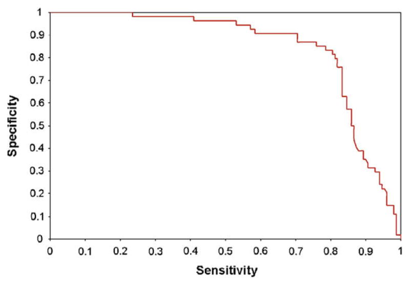
Sensitivity–specificity (ROC) curve for our logistic regression predictor on a set of literature-based interaction annotations (149 positive, 54 negative). Sensitivity, fraction of positive interactions that are predicted as positive. Specificity, fraction of negative interactions that are predicted as negative.

4.2. Graphic representation of protein–protein interactions

The assignment of IRS to individual protein–protein interactions and the selection of those interactions with IRS over a stringent threshold define high-confidence PPI datasets. Many different tools can be used to represent the data in a comprehensive manner. Here, we present two examples. Fig. 5 shows a graphical representation of part of our high-confidence interaction dataset in which edges that extend from a given bait are connected to the preys that have been confidently identified in our experiments. In this representation, which was generated using the VisANT software [19], the nodes have been clustered according to their GO annotation and/or the degree of connectivity between nodes. Fig. 4 shows a heat map where preys and baits are clustered based on the similarity of their sets of partners. Both Figs. 4 and 5 indicate the existence of the RPAP3 complex (R2TP/Prefoldin-like) and its tight connection to RNAPII and the CCT complex.

Fig. 5.

Network highlighting the composition of the RPAP3 (R2TP/prefoldin-like) complex (blue box). Subunit overlap with PFD (light blue box) and RNAP I, II and III (yellow box) is shown, as are interactions with RPAP2, RPAP4, RP11-529I10.4 (green nodes) and CCT complex (red box). Tagged proteins (baits) are in color, while untagged ones are represented in gray.

Fig. 4.

Heat map of a subset of our protein interaction network pertaining to the RPAP3 (R2TP/prefoldin-like) complex. For each pair bait/prey, the IRS is shown by color intensity (white being no interaction).

Appendix A. Supplementary data

Supplementary data associated with this article can be found, in the online version, at doi:10.1016/j.ymeth.2009.05.005.

References

- 1.Rigaut G, Shevchenko A, Rutz B, Wilm M, Mann M, Seraphin B. Nat Biotechnol. 1999;17:1030–1032. doi: 10.1038/13732. [DOI] [PubMed] [Google Scholar]
- 2.Puig O, Caspary F, Rigaut G, Rutz B, Bouveret E, Bragado-Nilsson E, Wilm M, Seraphin B. Methods. 2001;24:218–229. doi: 10.1006/meth.2001.1183. [DOI] [PubMed] [Google Scholar]
- 3.Florens L, Carozza MJ, Swanson SK, Fournier M, Coleman MK, Workman JL, Washburn MP. Methods. 2006;40:303–311. doi: 10.1016/j.ymeth.2006.07.028. [DOI] [PMC free article] [PubMed] [Google Scholar]
- 4.Ewing RM, Chu P, Elisma F, Li H, Taylor P, Climie S, McBroom-Cerajewski L, Robinson MD, O’Connor L, Li M, Taylor R, Dharsee M, Ho Y, Heilbut A, Moore L, Zhang S, Ornatsky O, Bukhman YV, Ethier M, Sheng Y, Vasilescu J, Abu-Farha M, Lambert JP, Duewel HS, Stewart II, Kuehl B, Hogue K, Colwill K, Gladwish K, Muskat B, Kinach R, Adams SL, Moran MF, Morin GB, Topaloglou T, Figeys D. Mol Syst Biol. 2007;3(89):1–17. doi: 10.1038/msb4100134. [DOI] [PMC free article] [PubMed] [Google Scholar]
- 5.Jeronimo C, Langelier MF, Zeghouf M, Cojocaru M, Bergeron D, Baali D, Forget D, Mnaimneh S, Davierwala AP, Pootoolal J, Chandy M, Canadien V, Beattie BK, Richards DP, Workman JL, Hughes TR, Greenblatt J, Coulombe B. Mol Cell Biol. 2004;24:7043–7058. doi: 10.1128/MCB.24.16.7043-7058.2004. [DOI] [PMC free article] [PubMed] [Google Scholar]
- 6.Jeronimo C, Forget D, Bouchard A, Li Q, Chua G, Poitras C, Therien C, Bergeron D, Bourassa S, Greenblatt J, Chabot B, Poirier GG, Hughes TR, Blanchette M, Price DH, Coulombe B. Mol Cell. 2007;27:262–274. doi: 10.1016/j.molcel.2007.06.027. [DOI] [PMC free article] [PubMed] [Google Scholar]
- 7.Krueger BJ, Jeronimo C, Roy BB, Bouchard A, Barrandon C, Byers SA, Searcey CE, Cooper JJ, Bensaude O, Cohen EA, Coulombe B, Price DH. Nucleic Acids Res. 2008;36:2219–2229. doi: 10.1093/nar/gkn061. [DOI] [PMC free article] [PubMed] [Google Scholar]
- 8.Gstaiger M, Luke B, Hess D, Oakeley EJ, Wirbelauer C, Blondel M, Vigneron M, Peter M, Krek W. Science. 2003;302:1208–1212. doi: 10.1126/science.1088401. [DOI] [PubMed] [Google Scholar]
- 9.Sardiu ME, Cai Y, Jin JJ, Swanson SK, Conaway RC, Conaway JW, Florens L, Washburn MP. Proc Natl Acad Sci USA. 2008;105:1454–1459. doi: 10.1073/pnas.0706983105. [DOI] [PMC free article] [PubMed] [Google Scholar]
- 10.Zhao RM, Davey M, Hsu YC, Kaplanek P, Tong A, Parsons AB, Krogan N, Cagney G, Mai D, Greenblatt J, Boone C, Emili A, Houry WA. Cell. 2005;120:715–727. doi: 10.1016/j.cell.2004.12.024. [DOI] [PubMed] [Google Scholar]
- 11.Zhao RM, Kakihara Y, Gribun A, Huen J, Yang GC, Khanna M, Costanzo M, Brost RL, Boone C, Hughes TR, Yip CM, Houry WA. J Cell Biol. 2008;180:563–578. doi: 10.1083/jcb.200709061. [DOI] [PMC free article] [PubMed] [Google Scholar]
- 12.Itsuki Y, Saeki M, Nakahara H, Egusa H, Irie Y, Terao Y, Kawabata S, Yatani H, Kamisaki Y. FEBS Lett. 2008;582:2365–2370. doi: 10.1016/j.febslet.2008.05.041. [DOI] [PubMed] [Google Scholar]
- 13.Dorjsuren D, Lin Y, Wei WX, Yamashita T, Nomura T, Hayashi N, Murakami S. Mol Cell Biol. 1998;18:7546–7555. doi: 10.1128/mcb.18.12.7546. [DOI] [PMC free article] [PubMed] [Google Scholar]
- 14.Djouder N, Metzler SC, Schmidt A, Wirbelauer C, Gstaiger M, Aebersold R, Hess D, Krek W. Mol Cell. 2007;28:28–40. doi: 10.1016/j.molcel.2007.08.010. [DOI] [PubMed] [Google Scholar]
- 15.Havlis J, Thomas H, Sebela M, Shevchenko A. Anal Chem. 2003;75:1300–1306. doi: 10.1021/ac026136s. [DOI] [PubMed] [Google Scholar]
- 16.Elias JE, Gygi SP. Nat Methods. 2007;4:207–214. doi: 10.1038/nmeth1019. [DOI] [PubMed] [Google Scholar]
- 17.Perkins DN, Pappin DJ, Creasy DM, Cottrell JS. Electrophoresis. 1999;20:3551–3567. doi: 10.1002/(SICI)1522-2683(19991201)20:18<3551::AID-ELPS3551>3.0.CO;2-2. [DOI] [PubMed] [Google Scholar]
- 18.Ashburner M, Ball CA, Blake JA, Botstein D, Butler H, Cherry JM, Davis AP, Dolinski K, Dwight SS, Eppig JT, Harris MA, Hill DP, Issel-Tarver L, Kasarskis A, Lewis S, Matese JC, Richardson JE, Ringwald M, Rubin GM, Sherlock G. Nat Genet. 2000;25:25–29. doi: 10.1038/75556. [DOI] [PMC free article] [PubMed] [Google Scholar]
- 19.Hu Z, Snitkin ES, DeLisi C. Brief Bioinform. 2008;9:317–325. doi: 10.1093/bib/bbn020. [DOI] [PMC free article] [PubMed] [Google Scholar]
Associated Data
This section collects any data citations, data availability statements, or supplementary materials included in this article.