Heterogeneous growth-induced prestrain in the heart

Abstract

Even when entirely unloaded, biological structures are not stress-free, as shown by Y.C. Fung’s seminal opening angle experiment on arteries and the left ventricle. As a result of this prestrain, subject-specific geometries extracted from medical imaging do not represent an unloaded reference configuration necessary for mechanical analysis, even if the structure is externally unloaded. Here we propose a new computational method to create physiological residual stress fields in subject-specific left ventricular geometries using the continuum theory of fictitious configurations combined with a fixed-point iteration. We also reproduced the opening angle experiment on four swine models, to characterize the range of normal opening angle values. The proposed method generates residual stress fields which can reliably reproduce the range of opening angles between 8.7±1.8 and 16.6 ± 13.7 as measured experimentally. We demonstrate that including the effects of prestrain reduces the left ventricular stiffness by up to 40%, thus facilitating the ventricular filling, which has a significant impact on cardiac function. This method can improve the fidelity of subject-specific models to improve our understanding of cardiac diseases and to optimize treatment options.

1. Introduction

Biological tissues inherently contain some prestrain, or equivalently residual stress (Vaishnav and Vossoughi, 1987; Fung, 1993; Humphrey, 2002). This has been evidenced in the opening angle experiments, performed originally on the artery in (Chuong and Fung, 1986), and then on the left ventricle in (Omens and Fung, 1990). The exact origin of the prestrain is still an open question: it may be induced by inhomogeneous tissue growth, or the constant exchange of matter within the tissues and associated remodeling, cell death, and renewal, etc. (Fung, 1993; Humphrey, 2002). Moreover, prestrain potentially exists across multiple spatial scales, including the sub-cellular (Kumar, Maxwell, et al., 2006; Deguchi, Ohashi and Sato, 2006), cellular, and structural levels (Fung, 1993; Humphrey, 2002; Guo, Lanir and Kassab, 2007).

It is important to distinguish between these different types of prestrain. Indeed, sub-cellular prestrain surely affects the response of individual cells, but is confined to the cells and cannot be characterized on the macroscopic level (Kumar, Maxwell, et al., 2006; Deguchi, Ohashi and Sato, 2006; Webster, Ng and Fletcher, 2014). Conversely, structural, or global, residual stress (imagine a stress-free straight beam glued into a circular shape for which a single cut would release all the residual stress at once) are most probably not seen in vivo. In support of this, while original experiments showed that the first cut released most of the residual stress (Liu and Fung, 1989; Han and Fung, 1996), later experiments revealed that subsequent cuts always release additional residual stress (Greenwald, Moore, et al., 1997). Hence, we investigate the prestrain generated on the cellular scale, a scale where living tissues are composed of many different components in frictional contact and constant relative motion. Cellular prestrain is analogous to the one present in engineering materials (e.g., between grains in metals) or between components in composites, which is usually induced by the process or differences in coefficients of thermal expansion. It is present everywhere in living systems and it can have a tremendous impact on their macroscopic behavior.

To address cardiovascular diseases, one approach is the use of personalized models for quantitative diagnostic, prognostic, and treatment optimization (Lee, Genet, et al., 2014b). The current bottlenecks in personalized cardiac modeling include the assessment of myofiber architecture (Toussaint, Stoeck, et al., 2013; Harmer, Pushparajah, et al., 2013), non-invasive pressure measurement, tissue properties orthotropy and regionality (Lee, Wenk, et al., 2011; Xi, Lamata, et al., 2011; Marchesseau, Delingette, et al., 2013). Another important limitation is our understanding of prestrain and residual stress. Indeed, as a result of prestrain, subject-specific geometries of biological structures extracted from medical imaging do not represent the reference configuration required for mechanical analysis, even if the images correspond to an externally unloaded state. To identify the truly unstressed reference configuration, we have to solve an inverse problem that is highly non-linear.

In this paper, we propose a computational method to introduce physiological residual stress fields in subject-specific left ventricular geometries. The proposed method is embedded within the continuum theory of fictitious configurations and uses a fixed-point iteration on the geometry itself. (Wang, Luo, et al., 2013) recently proposed an alternative approach, also using fixed-point iterations on the geometry to recover a relaxed configuration. However, they use (Shams, Destrade and Ogden, 2011)’s method to introduce residual stress in the invariant-based Holpzapfel model (Holzapfel and Ogden, 2009) through additional pseudo-invariants. This implies that (i) the method is limited to invariant-based formulations, (ii) that residual stress is introduced as an ad hoc parameter to fit experimental data (Costa, May-Newman, et al., 1997), and (iii) that the resulting residual stress field is not strictly speaking divergence free, i.e., auto-balanced. Here, the residual stress is generated mechanistically by the underlying biological process, heterogeneous growth, and is naturally auto-balanced.

2. Methods

2.1. Opening angle experiment

2.1.1. Animal preparation

We performed all animal experiments in accordance with national and local ethical guidelines, including the Principles of Laboratory Animal Care, the Guide for the Care and Use of Laboratory Animals (National Research Council (US) Committee for the Update of the Guide for the Care and Use of Laboratory Animals, 2011) and the National Association for Biomedical Research (Cardon, Bailey and Bennett, 2012), and an approved Indiana University Purdue University Indianapolis IACUC protocol regarding the use of animals in research. Four Yorkshire pigs (55.1 ± 3.0 Kg body weight) of either sex were used in this study. The pigs were fasted overnight and surgical anesthesia was induced with TKX (Telazol 10 mg/kg, Ketamine 5 mg/kg, Xylazine 5 mg/kg) and maintained with 1–2% Isoflurane-balance O₂ during acute, non-aseptic surgery. An introducer sheath was placed percutaneously in the right jugular vein for administration of drugs. The chest was opened through a mid-line sternotomy and the heart was arrested with an IV bolus injection of saturated KCl solution (20 mL) under deep anesthesia and proper anticoagulation with Heparin (100 IU/kg body weight).

2.1.2. Heart preparation

The heart was excised and placed in cardioplegic solution. We cannulated and perfused the left anterior descending, the left circumflex, and the right coronary arteries with a solution (Lin and Yin, 1998) of the following composition in mmol: NaCl, 127; KH2PO4, 1.3; MgSO4, 0.6; NaHCO3, 25; KCl, 2.3; CaCl2, 2.5; dextrose, 11.2; BDM (2,3 butanedione monoxime, Sigma, St. Louis, MO), 30. After perfusion, the aorta and pulmonary arteries, the right and left atria, and the right ventricular free wall were carefully cut, keeping an intact left ventricle in the shape of a cone.

2.1.3. Experimental procedure

After the first basal slice was discarded, three 1-cm-thick slices were cut from the left ventricle (basal, equatorial, and apical) and placed in petri dishes containing perfusion solution (see Figure 3). Two cameras were set up to photograph the cross-sectional surfaces of the slice from the top and the bottom surfaces simultaneously. A baseline picture was taken before a radial cut was made in the middle of the left ventricular free wall. Immediately after the cut was made, continuous pictures were taken every five minutes for a period of 30 minutes. The opening angle was measured with a program for image processing and analysis, ImageJ 1.44p (National Institutes of Health).

2.2. Mechanics of prestrained biological systems

2.2.1. Continuum model

We characterize prestrain using the concept of fictitious configurations and introduce a stress-free reference configuration, a residually stressed but mechanically unloaded configuration, and residually stressed mechanically loaded configuration (Rausch and Kuhl, 2013).

Figure 1 illustrates the three configurations, which can also be used to model prestrain induced by other physical mechanisms such as friction (Hild, 1998; Fagiano, Genet, et al., 2014). Under the small deformation hypothesis, this decomposition induces an additive decomposition of the strain itself: The total elastic strain is the sum of prestrain and mechanically-induced strain. Under finite deformations, this decomposition induces a multiplicative decomposition of the deformation gradient: The total elastic tensor $\underset{‗}{F^e}$ is the product of a prestrain tensor $\underset{‗}{F^p}$ and the mechanically-induced deformation gradient $\underset{‗}{F}$:

$$\underset{‗}{F^e}=\underset{‗}{F}·\underset{‗}{F^p}\text{with}\underset{‗}{F}=\underset{‗}{F^e}·{\underset{‗}{F}}^{p-1}=\nabla \underset{\_}{\phi }$$ (1)

Figure 1.

Kinematics of prestrained biological systems. Prestrain maps the stress-free reference configuration onto the residually stressed but mechanically unloaded configuration through the prestrain tensor $\underset{‗}{F^p}$. Mechanical loading maps the residually stressed but mechanically unloaded configuration into the mechanically loaded configuration through the deformation gradient $\underset{‗}{F}$. The total elastic deformation $\underset{‗}{F^e}$ is a result of prestrain $\underset{‗}{F^p}$ and mechanical deformation $\underset{‗}{F}$. Only the mechanical deformation $\underset{‗}{F}=\nabla \underset{\_}{\phi }$ is the gradient of a vector field, while the prestrain tensor $\underset{‗}{F^p}$ and the elastic tensor $\underset{‗}{F^e}$ are incompatible. Only the elastic tensor $\underset{‗}{F^e}$ generates stress.

Inherent to this approach, only the mechanically-induced deformation gradient $\underset{‗}{F}=\nabla \underset{\_}{\phi }$ is a gradient of a vector field, while $\underset{‗}{F^e}$ and $\underset{‗}{F^p}$ are generally incompatible. We can then adopt the classical finite deformation theory for nearly incompressible bodies (Holzapfel, 2000), however, now based on the total elastic tensor $\underset{‗}{F^e}$ instead of the purely mechanically-induced deformation gradient $\underset{‗}{F}$. This implies that we can express the strain energy potential, which is generally a function of $\underset{‗}{F}$ and $\underset{‗}{F^p}$ , as a function of $\underset{‗}{F^e}$ only:

$$\psi (\underset{‗}{F},\underset{‗}{F^p})={\psi }^e(\underset{‗}{F^e})$$ (2)

The most widely used method to impose incompressibility or quasi-incompressibility consists of further decomposing the elastic tensor into volumetric and isochoric parts:

$$\underset{‗}{F^e}=\underset{‗}{F^v}·\overline{\underset{‗}{F^e}}$$ (3)

with the volumetric contribution $\underset{‗}{F^v}={(J^e)}^{1/3}\underset{‗}{1}$ with $J^e=det(\underset{‗}{F^e})$ and the isochoric contribution $\overline{\underset{‗}{F^e}}={(J^e)}^{-1/3}\underset{‗}{F^e}$ so that $\overline{J^e}=det(\overline{\underset{‗}{F^e}})=1$. As a result of this decomposition, the independent variables are now the elastic Jacobian J^e and the isochoric elastic Cauchy-Green tensor $\overline{\underset{‗}{E^e}}$:

$$J^e=det(\underset{‗}{F^e})\text{and}\overline{\underset{‗}{E^e}}=\frac{1}{2}\left({\overline{\underset{‗}{F^e}}}^t·\overline{\underset{‗}{F^e}}-\underset{‗}{1}\right)$$ (4)

We can then split the elastic strain energy potential into volumetric and deviatoric parts:

$${\psi }^e(J^e,\overline{\underset{‗}{E^e}})=U(J^e)+\overline{{\psi }^e}(\overline{\underset{‗}{E^e}})$$ (5)

For the volumetric part of the strain energy function (Auricchio, Beirão da Veiga, et al., 2013), we could suggest the following expression:

$$U(J^e)=\frac{1}{D_0}\left(\frac{1}{2}({(J^e)}^2-1)-ln(J^e)\right)$$ (6)

For the deviatoric part, we use a transversely isotropic Fung law (Fung, 1993) adapted for myocardial tissue (Guccione, McCulloch and Waldman, 1991):

$$\overline{{\psi }^e}(\overline{\underset{‗}{E^e}})=\frac{1}{2}{C}_0\left(exp\left(\overline{\underset{‗}{E^e}}:\underset{‗}{\underset{‗}{B_0}}:\overline{\underset{‗}{E^e}}\right)-1\right)$$ (7)

where $\underset{‗}{\underset{‗}{B_0}}$ is a fourth-order constitutive tensor, which takes takes a diagonal format in Voigt notation (Mehrabadi and Cowin, 1990; François, 1995):

$$\widehat{\underset{‗}{B_0}}=\underset{‗}{\text{Diag}}(B_{ff},B_{ss},B_{nn},2B_{fs},2B_{fn},2B_{sn})$$ (8)

Its individual parameters B_ff, B_ss, B_nn, B_fs, B_fn, and B_sn weigh the influence of the normal fiber, sheet, and normal strains and of the corresponding shear components. Throughout this paper, we use the normal human myocardial properties characterized in (Genet, Lee, et al., 2014) and summarized in Table 1. Note that it is well-known that the Fung law is not poly-convex (Holzapfel, Gasser and Ogden, 2000; Holzapfel and Ogden, 2009), making the proposed model not strictly speaking thermodynamically consistent. However, it is still widely used for the myocardium; for this paper we solve our model implicitly and have not encountered any material instability. Furthermore, the framework presented here for growth-induced residual stress is independent from the choice of the strain energy potential, and a convex potential could be used instead.

Table 1.

Normal human myocardial properties (Genet, Lee, et al., 2014) used in this paper for the ventricular simulations.

D0 (kPa−1)	C0 (kPa)
10−3	0.115

Bff ()	Bss ()	Bnn ()	Bfs ()	Bfn ()	Bsn ()
14.4	5.76	5.76	5.04	5.04	2.88

These equations can, in principle, allow us to calculate the in vivo stress state of the heart. Unfortunately, however, neither the initial nor the grown configuration are known. Only the residually stressed mechanically unloaded configuration and the mechanically loaded configuration can be imaged in vivo. In what follows, we propose a fixed-point iteration to computationally retrieve the initial configuration from the in vivo-acquired configuration. The core assumption of this algorithm is that residual stresses are a result of biological growth.

2.2.2. Computational model

The constitutive laws have been implemented as a user subroutine into Abaqus/Standard. The subroutine is written in C++, and use the LMT++ library for linear algebra (Leclerc, 2010; Genet, 2010). The implementation is straightforward as outlined in detail in (Rausch and Kuhl, 2013).

2.3. Mechanics of growth-induced, prestrained biological systems

2.3.1. Continuum model

The origin of prestrain is still an open questions today. Here, we investigate the hypothesis that the prestrain is induced by heterogeneous growth. In order to model the growth of biological tissues, we once again adopt the concept of fictitious configurations and decompose the total deformation multiplicatively into elastic, prestrain, and growth parts (Rodriguez, Hoger and McCulloch, 1994; Ambrosi, Ateshian, et al., 2011; Kuhl, 2014). This decomposition is a very general tool, and can also be applied for instance to model tissue activation (Rossi, Ruiz-Baier, et al., 2012; Pezzuto, Ambrosi and Quarteroni, 2014)

Figure 2 shows the different configurations and transformations. Similar to the mechanics of prestrained biological systems in Section 2.2, the elastic tensor $\underset{‗}{F^e}$ can be multiplicatively decomposed into the prestrain $\underset{‗}{F^p}$ and the mechanically-induced deformation ${\underset{‗}{F}}^{\prime }$. Yet, we can also decompose the elastic tensor $\underset{‗}{F^e}$ into the inverse growth $\underset{‗}{F^g}$ and the deformation gradient $\underset{‗}{F}$:

$$\underset{‗}{F^e}={\underset{‗}{F}}^{\prime }·\underset{‗}{F^p}=\underset{‗}{F}·{\underset{‗}{F^g}}^{-1}\text{with}\underset{‗}{F}={\underset{‗}{F}}^{\prime }·\underset{‗}{F^p}·\underset{‗}{F^g}=\nabla \underset{\_}{\phi }$$ (9)

Figure 2.

Kinematics of growth-induced, prestrained biological systems. Growth turns the initial, stress-free and compatible configuration into the grown, stress-free but incompatible configuration. Prestrain maps the grown, stress-free configuration onto the residually stressed but mechanically unloaded configuration through the prestrain tensor $\underset{‗}{F^p}$. Mechanical loading maps the residually stressed but mechanically unloaded configuration into the mechanically loaded configuration through the deformation gradient ${\underset{‗}{F}}^{\prime }$. The total elastic deformation $\underset{‗}{F^e}$ is a result of prestrain $\underset{‗}{F^p}$ and mechanical deformation ${\underset{‗}{F}}^{\prime }$. The full deformation $\underset{‗}{F}$ is a result of growth $\underset{‗}{F^g}$, prestrain $\underset{‗}{F^p}$, and mechanical deformation ${\underset{‗}{F}}^{\prime }$. Only the full deformation $\underset{‗}{F}=\nabla \underset{\_}{\phi }$ and mechanically-induced deformation ${\underset{‗}{F}}^{\prime }=\nabla {\underset{\_}{\phi }}^{\prime }$ are gradients of a vector field, while the growth tensor $\underset{‗}{F^g}$, the prestrain tensor $\underset{‗}{F^p}$, and the elastic tensor $\underset{‗}{F^e}$ are incompatible. Note that Figure 2 becomes identical to Figure 1 if $\underset{‗}{F^g}=\underset{‗}{1}$.

Note that in the special case where $\underset{‗}{F}={\underset{‗}{F}}^{\prime }$, we have $\underset{‗}{F^p}={\underset{‗}{F^g}}^{-1}$. However, in practice we only work with $\underset{‗}{F^g}$, which obeys the evolution equation defined in the next paragraph, and $\underset{‗}{F^e}$, which contains both the prestrain F p and load-induced deformation ${\underset{‗}{F}}^{\prime }$, and is used to compute stress through the elastic strain energy potential. Figure 2 also illustrates the heterogeneous growth-induced prestrain map $\underset{‗}{F^p}$ between the incompatible grown configuration and the residually-stressed compatible configuration.

Here, in order to focus on growth-induced residual stress and not on the growth itself, we will use a simple isotropic and strain-driven growth law. Indeed, even though it is now established that maladaptive hypertrophic processes are largely anisotropic (Taber, 1995; Frey and Olson, 2003), physiological growth must involve both longitudinal and transverse growth, and isotropic growth is the simplest growth model that can generate residual stresses. Moreover, even though the hormonal mechanisms underlying tissue growth are complex and beyond the scope of this study, it is now accepted that hormonal signals are strongly regulated by mechanical signals, and that mechanotransduction, especially stretch-sensitivity, is one of the fundamental processes underlying tissue growth (Maillet, van Berlo and Molkentin, 2013). Note that elastic strain and stress are coupled through the constitutive relationship and not mutually independent, so a stress-driven law could be used as well. To characterize the kinematics of growth we can thus parameterize the growth tensor $\underset{‗}{F^g}$ in terms of a single scalar-valued growth multiplier ϑ^g:

$$\underset{‗}{F^g}={\vartheta }^g\underset{‗}{1}$$ (10)

To characterize the kinetics of growth, we assume that growth evolves in time according to the following evolution law:

$${\stackrel{.}{\vartheta }}^g=\frac{1}{\tau }\text{tr}(\underset{‗}{E^e})$$ (11)

where τ is a time constant for growth. Since it is the only time constant of the problem, we simply set it to 1, and consider all other time-dependent quantities in terms of it. This implies that the driving force for growth is the trace of the elastic deformation $\underset{‗}{E^e}$.

2.3.2. Computational model

Similar to the elasticity part in Section 2.2, we implemented the growth model as a user subroutine into the finite element package Abaqus/Standard. Since growth is driven by the elastic strains $\underset{‗}{E^e}$, which are in turn affected by growth as $\underset{‗}{F^e}=\underset{‗}{F}·{\underset{‗}{F^g}}^{-1}$, we iteratively determine the growth multiplier ϑ^g at the integration point level at every global iteration step. Rather than using a consistent Newton-Raphson procedure, which requires a consistent algorithmic linearization (Göktepe, Abilez and Kuhl, 2010; Göktepe, Abilez, et al., 2010), we adopt a local fixed-point iteration, supplemented by Aitken’s relaxation (Genet, Marcin and Ladeveze, 2013). For the time integration, we use an implicit mid-point rule. This results in the following algorithm to determine the local growth multiplier ϑ^g:

For a tolerance of tol = 10⁻⁶, the algorithm converges rapidly in only a few iterations.

2.3.3. Example of growth-induced, prestrained left ventricle

Throughout this paper, we will illustrate our proposed method on a patient-specific left ventricular model of a healthy human (Genet, Lee, et al., 2014). This model characterizes healthy human ventricular mechanics. Briefly, the geometry was extracted from magnetic resonance images by manual segmentation, and triangulated using linear hexahedrons. A generic myofiber orientation field, with linearly varying helix angle from +60° at the endocardium to −60° at the epicardium (Streeter and Bassett, 1966; Streeter, Spotnitz, et al., 1969), was assigned to the mesh. We use a standard displacement finite element method, with fully implicit time stepping. In terms of boundary conditions, we constrain normal displacement of the basal nodes, and apply pressure loading at the endocardial faces.

To introduce residual stresses in a subject-specific geometry, we solve the following problem: We load the left ventricle to a given ventricular pressure P̄, then keep the pressure constant for a time t̄ to allow the ventricle to grow, and then gradually remove the pressure. Growth duration t̄ is usually expressed as a function of the growth time constant τ, which is the only time constant of the problem. As a result of heterogeneous growth, the final configuration is unloaded, but not stress free, i.e., residually stressed. Our goal is now to iteratively determine the reference configuration for which the in vivo grown geometry for given a given P̄ and time t̄ matches our subject-specific imaging data. The following section describes how we identify the reference configuration using fixed-point iterations.

2.4. Computation of stress-free reference configuration of biological systems

2.4.1. Fixed-point iteration

As discussed in Section 2.3 and illustrated in Figure 2, the mechanically unloaded configuration from medical imaging is not a true reference configuration in the continuum mechanics sense since it is residually stressed. The stress free reference configuration is unknown and has to be determined iteratively. A common approach to this problem is to solve the so-called inverse elastic problem (Govindjee and Mihalic, 1996, 1998). Yet, this approach requires non-standard formulations and solvers on the continuum and discrete levels. Here we suggest an alternative fixed-point-based approach, which requires only modular modifications to the original forward problem. Fixed-point iterations have originally been proposed by (Sellier, 2011), and have recently been adopted for in the context of cardiac mechanics by (Wang, Gao, et al., 2013; Wang, Luo, et al., 2013; Krishnamurthy, Villongco, et al., 2013). However, previous approaches have only used the fixed-point iteration to identify the reference configuration associated with a loaded in vivo configuration. Here, we use it to find the reference configuration associated with an unloaded in vivo configuration. We assume that this unloaded structure contains heterogeneous growth-induced residual stresses.

Let X_ref denote the nodal positions of the residually stressed, mechanically unloaded configuration obtained, e.g., from in vivo imaging. The objective of the fixed-point iteration is to find the nodal positions X of the stress-free, incompatible configuration that will deform into X_ref through the loading-growth-unloading scenario described in Section 2.3. Similar to the fixed-point iteration solver used for the growth law in Section 2.3.2, we adopt Aitken’s relaxation (Aitken, 1950) to improve convergence. For time integration, we use here an implicit backward Euler scheme. The algorithm to iteratively determine the nodal positions X in the stress-free configuration looks as follows:

Here X_init are the initial nodal position of the stress-free reference configuration, and X_def are the deformed nodal position after the loading-growth-unloading procedure. This implies that X_init could, but does not have to, be equal to X_ref. Similar to the algorithm in Section 2.3.2, the fixed-point iteration converges rapidly in a few iterations for a tolerance of 10⁻¹ mm.

2.4.2. Computational model

We implemented the fixed-point iteration as a python script, which solves the growth problem inside the inner loop using Abaqus/Standard and then post-processes the nodal positions.

3. Results and Discussion

3.1. Opening angle experiment

Figure 3 illustrates our opening angle experiment. It shows an isolated heart slice before (left) and after (right) cutting the slice radially in the middle of the left ventricular free wall.

Figure 3.

Opening angle experiment. Isolated heart slice before (left) and after (right) radial cutting in the middle of the left ventricular free wall.

Table 2 summarizes the opening angles of the basal, equatorial, and apical slices of all four hearts. Average opening angles increase from base to apex (from 8.7° to 16.6°) with an increasing standard deviation (from ±1.8° to ±13.7°). The variability in opening angle may be attributed to a combination of geometric and structural differences between the two control slices, and the location of the radial cut. Nevertheless, opening angles are significantly lower than values found for rat hearts (45°) (Omens and Fung, 1990), hence potentially revealing a size-effect in residual stress development.

Table 2.

Opening angle experimental data. All values are reported in degrees.

	Basal slice	Equatorial slice	Apical slice
Heart 1	9.3	8.7	9.8
Heart 2	9.8	19.9	16.5
Heart 3	9.7	9.0	4.2
Heart 4	6.1	14.5	35.7
Mean±SD	8.7±1.8	13.0±5.3	16.6±13.7

3.2. Generating growth-induced prestrain

Figure 4 illustrates our protocol to generate prestrain through heterogeneous growth in a patient specific left ventricular geometry (Genet, Lee, et al., 2014). For the sake of illustration, we used a nominal ventricular pressure P̄ of 1 mmHg, and a nominal growth duration t̄ of one growth time constant τ. During the strain-driven growth step, the myofiber stress field becomes more and more homogeneous. While homogeneous isotropic growth does not generate residual stress, homogeneous anisotropic growth (Rausch, Dam, et al., 2011; Kerckhoffs, 2012) and heterogeneous isotropic growth (Göktepe, Abilez and Kuhl, 2010; Göktepe, Abilez, et al., 2010) do. Thus, the final configuration is residually stressed: the sub-endocardial region is in compression, the sub-epicardial region in in tension.

Figure 4.

Protocol to generate heterogeneous growth-induced residual stress in a patient specific left ventricular geometry. The ventricle is loaded to a ventricular pressure of P̄, (a)–(b), then allowed to grow for a duration t̄, (b)–(c), and then unloaded, (c)–(d). The strain-driven growth drives the growing configuration into a state with a more homogeneous myofiber stress and reduces regional stress variations (c). The final configuration is unloaded, but not stress free, with the sub-endocardial region in compression, and the sub-epicardial region in tension (d).

This is in contrast to some models in the literature (Kroon, Delhaas, et al., 2007, 2009), which hypothesize that the growth-induced residual stresses are relieved over time, such that the grown configuration is always assumed to be stress free. Our opening angle experiment indicates though that the inner layer of the ventricle, similar to arteries, is in compression and the outer layer is in tension. This result is compatible with strain-driven growth-induced prestrain, the underlying hypothesis in this paper.

We have used the trace of the elastic Green-Lagrange strain tensor as the thermodynamical force to drive growth. Other authors have used the fiber stretch (Lee, Genet, et al., 2014a); however, the fiber stretch is largest in the mid-wall and not in the sub-endocardial region (Choi, D’hooge, et al., 2010; Lee, Genet, et al., 2014a), and the associated residual stress fields are not physiological. Others have use the Kirchhoff (Klepach, Lee, et al., 2012) or Mandel (Göktepe, Abilez and Kuhl, 2010; Göktepe, Abilez, et al., 2010) stresses, which are more “isotropic” quantities. Actually, in the case of isotropic growth and compressible elasticity, the Mandel stress is the energy conjugate of the growth state variable; however, in the case of quasi-incompressible elasticity considered here, the energy conjugate of the isotropic growth state variable is basically the isostatic pressure, which does not seem to be a reasonable driving force. In other words, the distribution of residual stresses constrains the functional form of the growth law. This is why, after systematically testing a collection of other driving forces for growth, we decided to select the trace of the elastic deformation.

As for growth kinetic equation itself, for the lack of appropriate experiments, we use a simple linear evolution law. More complex evolution laws have been proposed, including thresholds and limiting values (Kuhl, 2014), and even multiple domains (Lee, Genet, et al., 2014a) to predict both growth and reverse growth. The growth law we have selected here is the simplest law to predict heterogeneous growth.

3.3. Growth-induced prestrain in patient-specific left ventricle

Figure 5 illustrates the fixed-point iteration method to solve for the reference configuration associated with a given amount of prestrain, once again generated with a nominal ventricular pressure of 1 mmHg and a nominal growth duration of one growth time constant. For each iteration (i.e., each column), we show the reference stress-free configuration (top row) and the final (after loading, growth, and unloading) configuration (bottom row). During the fixed-point iterations, we compute the error between the reference configuration (obtained from medical imaging) and the deformed configuration (after loading-growth-unloading). The very last geometry (last column, bottom row) is identical to the very first (first column, top row; this geometry is the in vivo unloaded geometry extracted from medical imaging), but it contains heterogeneous growth-induced residual stress.

Figure 5.

Fixed-point iteration method to compute the prestrained, mechanically unloaded reference configuration (last column, top row) so that the prestrained, mechanically loaded configuration (last column, bottom row) matches the in vivo geometry extracted from magnetic resonance images (first column, top row) but contains auto-balanced residual stresses.

Figure 6 shows, for multiple growth durations ranging from 1 to 6 growth time constants, the reference configuration computed using the fixed-point iteration method (top row) as well as the prestrained configuration. The reference configuration is always stress-free, but the geometry varies. On the contrary, the prestrained configuration has always the same geometry (the one extracted from medical imaging data), but different levels of residual stress.

Figure 6.

Prestrained configurations for varying prestrain levels. Prestrain is generated by heterogeneous growth. The reference configurations are computed using a fixed-point iteration, so that the prestrained configurations (bottom row) match the in vivo geometry extracted from magnetic resonance images (top row).

By assuming that the early-diastolic ventricular geometry extracted from medical imaging is unloaded, we implicitly neglected the ventricular pressure at the beginning of diastole. However, this hypothesis is not necessary for using the fixed-point iterations. In principle, it is possible to prescribe any loading at the end of the forward step of the inverse problem, thus taking into account the mechanical load applied to the tissues.

3.4. Virtual opening angle experiment

After generating residual stresses in the subject-specific left ventricular geometry, we slice the virtual heart longitudinally and then cut it open. The result is illustrated in Figure 7, for a nominal ventricular pressure of 1 mmHg, and a nominal growth duration of six growth time constants. To reproduce the experimental conditions, the nodes belonging to the upper and lower faces can only move in the sliding plane. To remove rigid body motions, the nodes of one face of the cut can only move in the cutting plane.

Figure 7.

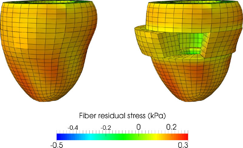
Virtual opening angle experiment. The prestrained configuration is sliced and then cut. The slice naturally springs open, similar to the physical experiment illustrated in Figure 3. Cutting the slice relieves some, but not all residual stress. Colors represent residual fiber stress, in kPa.

Figure 8 shows the relationship between the maximum principal residual strain in the slice and the opening angle. Different levels of residual strain are generated using different growth durations, ranging from 1 to 6 growth time constants, while a 1 mmHg ventricular pressure is always used. The black line and the gray box mark the average and standard deviation from the physical opening angle experiment on the mid-level slice in Section 3.1.

Figure 8.

Opening angles for varying prestrain levels. The green curve summarizes the computationally simulated opening angles for a pressure of P̄ = 1 mmHg. The black line and gray box mark the experimentally measured opening angle of 13±5.3° for the equatorial slice. Computationally simulated opening angles lie within the range of experimentally measured opening angles.

It is not necessary to shrink the ventricle to an infinitesimally small size to then induce enough residual stress through growth to generate a realistic opening angle. Our proposed method thus allows us to distinguish between the residual stress that is released, and the residual stress that remains within the tissues. Moreover, the fact that some of the residual stress is released justifies the original assumption that there exists a stress-free compatible configuration, which is described in Figure 2, and computed using the fixed-point algorithm described Section 2.4.

3.5. Influence of the prestrain on the ventricular mechanical response

An important consequence of prestrain is the influence of the residual stress on the mechanical response of the heart. Figure 9 shows the passive pressure-volume relationship for different levels of prestrain associated with different opening angles. Once again, the different levels of prestrain are generated using different growth durations, here ranging from 1 to 6 growth time constants, and the ventricular pressure during growth is kept constant a 1 mmHg. Because of the nature of residual stresses in growing circular cross sections, with compressive stresses at the sub-endocardial region and tensile stresses at the sub-epicardial region, prestrain tends to make the ventricle more compliant. For instance, for a maximal principal prestrain of 15.34%, a fiber residual stress varying from −0.12kPa to +0.055kPa, and an opening angle of 17.1°, i.e., close to the average experimental value, the ventricular pressure after a passive filling corresponding to an unloaded ventricular volume (i.e., a 50% ejection fraction) is reduced by 25.8% compared to the prestrain-free ventricle. As a consequence of this increased compliance, the ventricle requires less energy to fill. In other words, besides the well-known effect of homogenizing the ventricular wall stress (Omens and Fung, 1990), residual stresses could be a mechanism to directly improve ventricular diastolic function.

Figure 9.

Passive pressure-volume response of the left ventricle for varying prestrain levels. Increasing the prestrain level increases the ventricular compliance: for an opening angle of 17.1°, i.e., close to the average experimental value, the ventricular pressure after passive filling corresponding to a 50% ejection fraction is reduced by 25.8% compared to the prestrain-free case.

4. Summary and Perspectives

In this paper, we investigated the hypothesis that residual stress in the beating heart is induced by growth of the organ. We used the finite growth framework, together with a fixed-point iteration on the geometry itself, to introduce residual stress in a subject-specific left ventricular geometry. We showed that the residual stress fields induced by heterogeneous growth are compatible with experimental results, both qualitatively and quantitatively. It can successfully predict the physiological range of opening angles. We showed that the prestrain can have a significant impact on the passive mechanical response of the ventricle, making it much more compliant.

Some more general perspectives follow from this work. First, in addition to studying the influence of the prestrain on the passive ventricular response alone, we will characterize the sensitivity of the active response, and, eventually, of the entire pressure-volume relationship, for different prestrain levels. Another important follow up study will be to incorporate the algorithm introduced here within a personalized left ventricular model (Genet, Lee, et al., 2014), and compute personalized passive and active cardiac mechanical properties by taking into account physiological prestrain levels. Finally, we will study the interactions between physiological residual stress and residual stress induced by the injection of biomaterials in diseased myocardium as a potential treatments (Lee, Wall, et al., 2013, 2014), and their respective influence on ventricular mechanics. We believe that prestrain could be the key to explain various discrepancies in the literature between in vivo and ex vivo measurements and computational simulations. Including the effects of prestrain have the potential to make subject-specific modeling more reliable and more applicable to today’s cardiac health problems.

References

- Aitken AC. On the Iterative Solution of a System of Linear Equations. Proceedings of the Royal Society of Edinburgh Section A Mathematical and Physical Sciences. 1950;63(01):52–60. Available from: http://journals.cambridge.org/abstract_S008045410000697X. [Google Scholar]
- Ambrosi D, Ateshian GA, Arruda EM, Cowin SC, Dumais J, Goriely A, Holzapfel GA, Humphrey JD, Kemkemer R, Kuhl E, et al. Perspectives on biological growth and remodeling. Journal of the mechanics and physics of solids. 2011;59(4):863–883. doi: 10.1016/j.jmps.2010.12.011. [DOI] [PMC free article] [PubMed] [Google Scholar]
- Auricchio F, Beirão da Veiga L, Lovadina C, Reali A, Taylor RL, Wriggers P. Approximation of incompressible large deformation elastic problems: some unresolved issues. Computational Mechanics. 2013;52(5):1153–1167. Available from: http://link.springer.com/10.1007/s00466-013-0869-0. [Google Scholar]
- Cardon AD, Bailey MR, Bennett BT. The Animal Welfare Act: from enactment to enforcement. Journal of the American Association for Laboratory Animal Science. 2012;51:301–5. Available from: http://www.pubmedcentral.nih.gov/articlerender.fcgi?artid=3358977&tool=pmcentrez&rendertype=abstract. [PMC free article] [PubMed] [Google Scholar]
- Choi HF, D’hooge J, Rademakers FE, Claus P. Influence of left-ventricular shape on passive filling properties and end-diastolic fiber stress and strain. Journal of biomechanics. 2010;43(9):1745–53. doi: 10.1016/j.jbiomech.2010.02.022. Available from: http://www.ncbi.nlm.nih.gov/pubmed/20227697. [DOI] [PubMed] [Google Scholar]
- Chuong CJ, Fung YC. Residual stress in arteries. In: Schmid-Schönbein GW, Woo SLY, Zweifach BW, editors. Frontiers in biomechanics. New York, NY: Springer New York; 1986. [Google Scholar]
- Costa KD, May-Newman K, Farr D, O’Dell WG, McCulloch AD, Omens JH. Three-dimensional residual strain in midanterior canine left ventricle. The American journal of physiology. 1997;273:H1968–H1976. doi: 10.1152/ajpheart.1997.273.4.h1968. [DOI] [PMC free article] [PubMed] [Google Scholar]
- Deguchi S, Ohashi T, Sato M. Tensile properties of single stress fibers isolated from cultured vascular smooth muscle cells. Journal of biomechanics. 2006;39(14):2603–10. doi: 10.1016/j.jbiomech.2005.08.026. Available from: http://www.jbiomech.com/article/S002192900500401X/fulltext. [DOI] [PubMed] [Google Scholar]
- Fagiano C, Genet M, Baranger E, Ladevèze P. Computational geometrical and mechanical modeling of woven ceramic composites at the mesoscale. Composite Structures. 2014;112:146–156. Available from: http://linkinghub.elsevier.com/retrieve/pii/S0263822314000646. [Google Scholar]
- François M. Identification des symetries materielles de materiaux anisotropes [dissertation] Université Pierre et Marie Curie; Paris VI: 1995. [Google Scholar]
- Frey N, Olson EN. Cardiac hypertrophy: the good, the bad, and the ugly. Annual review of physiology. 2003;65:45–79. doi: 10.1146/annurev.physiol.65.092101.142243. Available from: http://www.ncbi.nlm.nih.gov/pubmed/12524460. [DOI] [PubMed] [Google Scholar]
- Fung YC. Biomechanics: Mechanical properties of living tissues. Springer; 1993. [Google Scholar]
- Genet M. Phd thesis. ENS-Cachan; 2010. Toward a virtual material for ceramic composites (in French) [Google Scholar]
- Genet M, Lee LC, Nguyen R, Haraldsson H, Acevedo-Bolton G, Zhang Z, Ge L, Ordovas K, Kozerke S, Guccione JM. Distribution of normal human left ventricular myofiber stress at end-diastole and end-systole—a target for in silico studies of cardiac procedures. Journal of Applied Physiology. 2014;117:142–52. doi: 10.1152/japplphysiol.00255.2014. [DOI] [PMC free article] [PubMed] [Google Scholar]
- Genet M, Marcin L, Ladeveze P. On structural computations until fracture based on an anisotropic and unilateral damage theory. International Journal of Damage Mechanics. 2013;23(4):483–506. Available from: http://ijd.sagepub.com/cgi/doi/10.1177/1056789513500295. [Google Scholar]
- Göktepe S, Abilez OJ, Kuhl E. A generic approach towards finite growth with examples of athlete’s heart, cardiac dilation, and cardiac wall thickening. Journal of the Mechanics and Physics of Solids. 2010;58(10):1661–1680. [Google Scholar]
- Göktepe S, Abilez OJ, Parker KK, Kuhl E. A multiscale model for eccentric and concentric cardiac growth through sarcomerogenesis. Journal of Theoretical Biology. 2010;265(3):433–42. doi: 10.1016/j.jtbi.2010.04.023. [DOI] [PubMed] [Google Scholar]
- Govindjee S, Mihalic PA. Computational methods for inverse finite elastostatics. Computer Methods in Applied Mechanics and Engineering. 1996;136(1–2):47–57. Available from: http://linkinghub.elsevier.com/retrieve/pii/0045782596010456. [Google Scholar]
- Govindjee S, Mihalic PA. Computational methods for inverse deformations in quasi-incompressible finite elasticity. International Journal for Numerical Methods in Engineering. 1998;43(5):821–838. [Google Scholar]
- Greenwald SE, Moore JE, Rachev A, Kane TPC, Meister JJ. Experimental Investigation of the Distribution of Residual Strains in the Artery Wall. Journal of Biomechanical Engineering. 1997;119(4):438. doi: 10.1115/1.2798291. Available from: http://biomechanical.asmedigitalcollection.asme.org/article.aspx?articleid=1400949. [DOI] [PubMed] [Google Scholar]
- Guccione JM, McCulloch AD, Waldman LK. Passive material properties of intact ventricular myocardium determined from a cylindrical model. Journal of Biomechanical Engineering. 1991;113(1):42–55. doi: 10.1115/1.2894084. [DOI] [PubMed] [Google Scholar]
- Guo X, Lanir Y, Kassab GS. Effect of osmolarity on the zero-stress state and mechanical properties of aorta. American journal of physiology: Heart and circulatory physiology. 2007;293:H2328–H2334. doi: 10.1152/ajpheart.00402.2007. [DOI] [PubMed] [Google Scholar]
- Han HC, Fung YC. Direct measurement of transverse residual strains in aorta. The American Journal of Physiology. 1996;270:H750–H759. doi: 10.1152/ajpheart.1996.270.2.H750. [DOI] [PubMed] [Google Scholar]
- Harmer J, Pushparajah K, Toussaint N, Stoeck CT, Chan RW, Atkinson D, Razavi R, Kozerke S. In vivo myofibre architecture in the systemic right ventricle. European heart journal. 2013;34(47):3640. doi: 10.1093/eurheartj/eht442. Available from: http://eurheartj.oxfordjournals.org/content/34/47/3640.shorthttp://www.ncbi.nlm.nih.gov/pubmed/24142348. [DOI] [PubMed] [Google Scholar]
- Hild F. Habilitation thesis. Pierre and Marie Curie University—Paris; 1998. Damage, Failure and Scale Bridging in Heterogeneous Materials (in French) p. 6. [Google Scholar]
- Holzapfel GA. Nonlinear Solid Mechanics: A Continuum Approach for Engineering. Wiley; 2000. [Google Scholar]
- Holzapfel GA, Gasser TC, Ogden RW. A new constitutive framework for arterial wall mechanics and a comparative study of material models. Journal of Elasticity. 2000;61:1–48. [Google Scholar]
- Holzapfel GA, Ogden RW. Constitutive modelling of passive myocardium: a structurally based framework for material characterization. Philosophical transactions of the Royal Society A: Mathenatical, Physical & Engineering Sciences. 2009;367(1902):3445–75. doi: 10.1098/rsta.2009.0091. Available from: http://www.ncbi.nlm.nih.gov/pubmed/19657007. [DOI] [PubMed] [Google Scholar]
- Humphrey JD. Cardiovascular Solid Mechanics: Cells, Tissues, and Organs. Springer-Verlag; 2002. [Google Scholar]
- Kerckhoffs RCP. Computational modeling of cardiac growth in the post-natal rat with a strain-based growth law. Journal of Biomechanics. 2012;45(5):865–71. doi: 10.1016/j.jbiomech.2011.11.028. Available from: http://www.pubmedcentral.nih.gov/articlerender.fcgi?artid=3294007&tool=pmcentrez&rendertype=abstract. [DOI] [PMC free article] [PubMed] [Google Scholar]
- Klepach D, Lee LC, Wenk JF, Ratcliffe MB, Zohdi TI, Navia JA, Kassab GS, Kuhl E, Guccione JM. Growth and remodeling of the left ventricle: A case study of myocardial infarction and surgical ventricular restoration. Mechanics Research Communications. 2012;42:134–141. doi: 10.1016/j.mechrescom.2012.03.005. [DOI] [PMC free article] [PubMed] [Google Scholar]
- Krishnamurthy A, Villongco CT, Chuang J, Frank LR, Nigam V, Belezzuoli E, Stark P, Krummen DE, Narayan SM, Omens JH, et al. Patient-Specific Models of Cardiac Biomechanics. Journal of computational physics. 2013;244:4–21. doi: 10.1016/j.jcp.2012.09.015. Available from: http://www.pubmedcentral.nih.gov/articlerender.fcgi?artid=3667962&tool=pmcentrez&rendertype=abstract. [DOI] [PMC free article] [PubMed] [Google Scholar]
- Kroon W, Delhaas T, Arts T, Bovendeerd PHM. Constitutive Modeling of Cardiac Tissue Growth. FIMH 2007. 2007:340–349. [Google Scholar]
- Kroon W, Delhaas T, Arts T, Bovendeerd PHM. Computational modeling of volumetric soft tissue growth: Application to the cardiac left ventricle. Biomechanics and Modeling in Mechanobiology. 2009;8:301–309. doi: 10.1007/s10237-008-0136-z. [DOI] [PubMed] [Google Scholar]
- Kuhl E. Growing matter: A review of growth in living systems. Journal of the Mechanical Behavior of Biomedical Materials. 2014;29:529–543. doi: 10.1016/j.jmbbm.2013.10.009. [DOI] [PubMed] [Google Scholar]
- Kumar S, Maxwell IZ, Heisterkamp A, Polte TR, Lele TP, Salanga M, Mazur E, Ingber DE. Viscoelastic retraction of single living stress fibers and its impact on cell shape, cytoskeletal organization, and extra-cellular matrix mechanics. Biophysical Journal. 2006;90(10):3762–73. doi: 10.1529/biophysj.105.071506. Available from: http://www.pubmedcentral.nih.gov/articlerender.fcgi?artid=1440757&tool=pmcentrez&rendertype=abstract. [DOI] [PMC free article] [PubMed] [Google Scholar]
- Leclerc H. In: Allix O, Wriggers P, editors. Towards a no compromise approach between modularity, versatility and execution speed for computational mechanics on CPUs and GPUs; IV European Conference on Computational Mechanics (ECCM2010); Paris, France. 2010. [Google Scholar]
- Lee LC, Genet M, Acevedo-Bolton G, Ordovas K, Guccione JM, Kuhl E. A computational model that predicts reverse growth in response to mechanical unloading. Biomechanics and modeling in mechanobiology. 2014a doi: 10.1007/s10237-014-0598-0. Available from: http://www.ncbi.nlm.nih.gov/pubmed/24888270. [DOI] [PMC free article] [PubMed]
- Lee LC, Genet M, Dang AB, Ge L, Guccione JM, Ratcliffe MB. Applications of computational modeling in cardiac surgery. Journal of Cardiac Surgery. 2014b;29(3):293–302. doi: 10.1111/jocs.12332. [DOI] [PMC free article] [PubMed] [Google Scholar]
- Lee LC, Wall ST, Genet M, Hinson A, Guccione JM. Bioinjection treatment: Effects of post-injection residual stress on left ventricular wall stress. Journal of Biomechanics. 2014;47(12):3115–9. doi: 10.1016/j.jbiomech.2014.06.026. [DOI] [PMC free article] [PubMed] [Google Scholar]
- Lee LC, Wall ST, Klepach D, Ge L, Zhang Z, Lee RJ, Hinson A, Gorman JH, Gorman RC, Guccione JM. Algisyl-LVR™ with coronary artery bypass grafting reduces left ventricular wall stress and improves function in the failing human heart. International Journal of Cardiology. 2013:1–7. doi: 10.1016/j.ijcard.2013.01.003. [DOI] [PMC free article] [PubMed] [Google Scholar]
- Lee LC, Wenk JF, Klepach D, Zhang Z, Saloner D, Wallace AW, Ge L, Ratcliffe MB, Guccione JM. A Novel Method for Quantifying In-Vivo Regional Left Ventricular Myocardial Contractility in the Border Zone of a Myocardial Infarction. 2011. [DOI] [PMC free article] [PubMed] [Google Scholar]
- Lin DH, Yin FC. A multiaxial constitutive law for mammalian left ventricular myocardium in steady-state barium contracture or tetanus. Journal of biomechanical engineering. 1998;120:504–517. doi: 10.1115/1.2798021. [DOI] [PubMed] [Google Scholar]
- Liu SQ, Fung YC. Relationship between hypertension, hypertrophy, and opening angle of zero-stress state of arteries following aortic constriction. Journal of Biomechanical Engineering. 1989;111:325–335. doi: 10.1115/1.3168386. [DOI] [PubMed] [Google Scholar]
- Maillet M, van Berlo JH, Molkentin JD. Molecular basis of physiological heart growth: fundamental concepts and new players. Nature reviews Molecular cell biology. 2013;14(1):38–48. doi: 10.1038/nrm3495. Available from: http://www.ncbi.nlm.nih.gov/pubmed/23258295. [DOI] [PMC free article] [PubMed] [Google Scholar]
- Marchesseau S, Delingette H, Sermesant M, Cabrera-Lozoya R, Tobon-Gomez C, Moireau P, Figueras i Ventura RM, Lekadir K, Hernandez A, Garreau M, et al. Personalization of a cardiac electromechanical model using reduced order unscented Kalman filtering from regional volumes. Medical image analysis. 2013;17(7):816–29. doi: 10.1016/j.media.2013.04.012. Available from: http://www.sciencedirect.com/science/article/pii/S1361841513000650http://hal.inria.fr/hal-00819806http://www.ncbi.nlm.nih.gov/pubmed/23707227. [DOI] [PubMed] [Google Scholar]
- Mehrabadi M, Cowin SC. Eigentensors of linear anisotropic elastic materials. The Quarterly Journal of Mechanics and Applied Mathematics. 1990;43(1) Available from: http://qjmam.oxfordjournals.org/content/43/1/15.short. [Google Scholar]
- National Research Council (US) Committee for the Update of the Guide for the Care and Use of Laboratory Animals. Guide for the Care and Use of Laboratory Animals. 8 2011. [Google Scholar]
- Omens JH, Fung YC. Residual strain in rat left ventricle. Circulation Research. 1990;66(1):37–45. doi: 10.1161/01.res.66.1.37. Available from: http://circres.ahajournals.org/content/66/1/37.short. [DOI] [PubMed] [Google Scholar]
- Pezzuto S, Ambrosi D, Quarteroni A. An orthotropic active–strain model for the myocardium mechanics and its numerical approximation. European Journal of Mechanics - A/Solids. 2014 Available from: http://www.sciencedirect.com/science/article/pii/S0997753814000527.
- Rausch MK, Dam A, Göktepe S, Abilez OJ, Kuhl E. Computational modeling of growth: systemic and pulmonary hypertension in the heart. Biomechanics and Modeling in Mechanobiology. 2011;10(6):799–811. doi: 10.1007/s10237-010-0275-x. [DOI] [PMC free article] [PubMed] [Google Scholar]
- Rausch MK, Kuhl E. On the effect of prestrain and residual stress in thin biological membranes. Journal of the Mechanics and Physics of Solids. 2013 doi: 10.1016/j.jmps.2013.04.005. [DOI] [PMC free article] [PubMed] [Google Scholar]
- Rodriguez EK, Hoger A, McCulloch AD. Stress-dependent finite growth in soft elastic tissues. Journal of Biomechanics. 1994;27(4):455–467. doi: 10.1016/0021-9290(94)90021-3. [DOI] [PubMed] [Google Scholar]
- Rossi S, Ruiz-Baier R, Pavarino LF, Quarteroni A. Orthotropic active strain models for the numerical simulation of cardiac biomechanics. International Journal for Numerical Methods in Biomedical Engineering. 2012;28(6–7):761–788. doi: 10.1002/cnm.2473. Available from: http://doi.wiley.com/10.1002/cnm.2473. [DOI] [PubMed] [Google Scholar]
- Sellier M. An iterative method for the inverse elasto-static problem. Journal of Fluids and Structures. 2011;27(8):1461–1470. [Google Scholar]
- Shams M, Destrade M, Ogden RW. Initial stresses in elastic solids: Constitutive laws and acoustoelasticity. Wave Motion. 2011;48:552–567. [Google Scholar]
- Streeter DD, Bassett DL. An engineering analysis of myocardial fiber orientation in pig’s left ventricle in systole. The Anatomical Record. 1966;155(4):503–511. [Google Scholar]
- Streeter DD, Spotnitz HM, Patel DP, Ross J, Sonnenblick EH. Fiber orientation in the canine left ventricle during diastole and systole. Circulation research. 1969;24(3):339–47. doi: 10.1161/01.res.24.3.339. [DOI] [PubMed] [Google Scholar]
- Taber LA. Biomechanics of Growth, Remodeling, and Morphogenesis. Applied Mechanics Reviews. 1995;48(8):487. Available from: http://appliedmechanicsreviews.asmedigitalcollection.asme.org/article.aspx?articleid=1395451. [Google Scholar]
- Toussaint N, Stoeck CT, Sermesant M, Schaeffter T, Kozerke S, Batchelor PG. In vivo human cardiac fibre architecture estimation using shape-based diffusion tensor processing. Medical Image Analysis. 2013 doi: 10.1016/j.media.2013.02.008. Available from: http://www.ncbi.nlm.nih.gov/pubmed/23523287. [DOI] [PubMed]
- Vaishnav RN, Vossoughi J. Residual stress and strain in aortic segments. Journal of biomechanics. 1987;20:235–239. doi: 10.1016/0021-9290(87)90290-9. [DOI] [PubMed] [Google Scholar]
- Wang HM, Gao H, Luo XY, Berry C, Griffith BE, Ogden RW, Wang TJ. Structure-based finite strain modelling of the human left ventricle in diastole. International journal for numerical methods in biomedical engineering. 2013;29(1):83–103. doi: 10.1002/cnm.2497. Available from: http://www.ncbi.nlm.nih.gov/pubmed/23293070. [DOI] [PubMed] [Google Scholar]
- Wang HM, Luo XY, Gao H, Ogden RW, Griffith BE, Berry C, Wang TJ. A modified Holzapfel-Ogden law for a residually stressed finite strain model of the human left ventricle in diastole. Biomechanics and modeling in mechanobiology. 2013 doi: 10.1007/s10237-013-0488-x. Available from: http://www.ncbi.nlm.nih.gov/pubmed/23609894. [DOI] [PMC free article] [PubMed]
- Webster KD, Ng WP, Fletcher DA. Tensional homeostasis in single fibroblasts. Biophysical Journal. 2014;107(1):146–55. doi: 10.1016/j.bpj.2014.04.051. Available from: http://www.ncbi.nlm.nih.gov/pubmed/24988349. [DOI] [PMC free article] [PubMed] [Google Scholar]
- Xi J, Lamata P, Lee J, Moireau P, Chapelle D, Smith NP. Myocardial transversely isotropic material parameter estimation from in-silico measurements based on a reduced-order unscented Kalman filter. Journal of the mechanical behavior of biomedical materials. 2011;4(7):1090–102. doi: 10.1016/j.jmbbm.2011.03.018. Available from: http://www.ncbi.nlm.nih.gov/pubmed/21783118. [DOI] [PubMed] [Google Scholar]