Exploring the inequality-mortality relationship in the US with Bayesian spatial modeling

Abstract

While there is evidence to suggest that socioeconomic inequality within places is associated with mortality rates among people living within them, the empirical connection between the two remains unsettled as potential confounders associated with racial and social structure are overlooked. This study seeks to test this relationship, to determine whether it is due to differential levels of deprivation and social capital, and does so with intrinsically conditional autoregressive Bayesian spatial modeling that effectively addresses the bias introduced by spatial dependence. We find that deprivation and social capital partly but not completely account for why inequality is positively associated with mortality and that spatial modeling generates more accurate predictions than does the traditional approach. We advance the literature by unveiling the intervening roles of social capital and deprivation in the inequality-mortality relationship and offering new evidence that inequality matters in US county mortality rates.

1. Introduction

Does income inequality threaten population health? Despite ecological evidence that inequality is associated with higher mortality in the US, for at least three reasons uncertainties remain (Lynch, Smith, Harper, Hillemeier, et al., 2004; Wilkinson & Pickett, 2006). First, the strength of prevailing evidence varies by geographic scale, with state-level analyses more supportive than county-level findings (Wilkinson & Pickett, 2006). Inequality is better captured with state-level than with county-level data (Wilkinson & Pickett, 2006, 2009) because income distributions are generally wider within states than counties. Regardless, the inconsistent evidence by scale of analysis suggests that data aggregation bias may plague studies in this area (Deaton & Lubotsky, 2003). Recently, it has been argued that “county” is a more appropriate analytic unit than “state” as it accounts for the heterogeneity within a state, which helps to study spatial inequality in detail, and has more relevant implications for localities (Lobao, Hooks, & Tickamyer, 2007). Accordingly, this study will analyze county-level data.

Second, it has been argued that the inequality-mortality association is unique to the US because inequality is a proxy for the race and social structure of this country (Deaton & Lubotsky, 2003; Ross et al., 2000). As minority groups in the US are more likely to be impoverished and live in socially disorganized areas, the inequality-mortality relationship may be attributed to social and political structure. Hence, controlling for these factors should eliminate the inequality-mortality relationship (Deaton, 2001, 2003). For example, African Americans suffer greater socioeconomic deprivation and often reside in high-poverty environments marked by social disorganization, which together create health disparities (Kawachi & Kennedy, 1997b; Williams, Mohammed, Leavell, & Collins, 2010). Specifically, areas that are socially disorganized would experience more crime and do not permit growth of social ties/capital and local attachment because social spaces would be characterized by social problems, such as violence and poverty (Taylor, 1996). Though these factors have been suggested to account for the inequality-mortality relationship (Kawachi, Kennedy, Lochner, & Prothrow-Stith, 1997; Singh, 2003), relatively few studies have systematically argued how and why these factors matter and, to our knowledge, no one has attempted to untangle the intertwined relationships among inequality, deprivation, social capital, and mortality.

Third, methodologically, previous ecological studies have often used simple bivariate analysis, as opposed to more rigorous multivariate modeling that can yield unbiased estimates and more decisive evidence (Deaton, 2003). Fewer studies still consider the spatial structure underlying the data and spatial dependence which may bias statistical estimates and generate misleading conclusions (Cressie, 1993; Haining, 2003; Voss, Long, Hammer, & Friedman, 2006). Spatial analysis approaches that contend with spatial dependence have been uncommon in mortality research until recently (McLaughlin, Stokes, Smith, & Nonoyama, 2007; Sparks & Sparks, 2010; Yang, Jensen, & Haran, 2011; Yang, Teng, & Haran, 2009), and this work does not focus on income inequality.

Cognizant of these sources of uncertainty, this study endeavors to contribute to the inequality-mortality question by providing theoretical arguments as to why deprivation and social capital could account for the inequality-mortality relationship, exploring these arguments empirically using county-level data which have tended to yield weaker results, and testing them with a Bayesian spatial approach that minimizes the bias caused by spatial dependence.

2. Research Framework

2.1. Intervening factors between inequality and mortality

We consider two basic mechanisms linking inequality and mortality. The first mechanism (psychosocial pathway) is that a sense of deprivation and disadvantage increases with inequality, and these psychosocial burdens lead to emotional problems (e.g., depression and hostility), risky behaviors (e.g., smoking and excessive drinking), and other manifestations of stress that compromise individual health and increase mortality (Marmot, 2004; Wilkinson, 2006). More explicitly, high inequality awakens the poor to the sense of being deprived because of the lack of resources and options that are related to one's social position in contrast to the rich. Without the ability to alleviate deprivation, this psychosocial pathway may provide an explanation why the deprived consistently show worse health than their counterparts (Marmot, 2004). Accordingly, the inclusion of deprivation should, theoretically and empirically, help account for the inequality-mortality relationship. While Deaton (2001) attempted to explore the role of deprivation in mortality, several important covariates at the aggregate-level that may affect the psychosocial pathway, such as social capital, were not considered in his analysis.

Deprivation is simply the state of lacking resources and opportunities in a specified area (Bartley & Blane, 1994; Buckingham & Freeman, 1997), and has been used to explain mortality differentials worldwide (Phillimore, Beattie, & Townsend, 1994; Singh, 2003; Singh & Siahpush, 2006; Townsend, Phillimore, & Beattie, 1988). Specifically, since the 1980s, area-based deprivation has been found to well explain the mortality differential across space, leading to suggestions for its use as a key variable in health research (Carstairs & Morris, 1989; Rey, Jougla, Fouillet, & Hémon, 2009). Nonetheless, deprivation has not been visible in the literature, and including it will help evaluate whether inequality affects mortality via the psychosocial pathway.

The second mechanism (underinvestment pathway) is that high inequality leads to underinvestment in social capital, civic resources, and other social environmental factors in a community (Daly, Duncan, Kaplan, & Lynch, 1998; Kawachi et al., 1997; Lynch & Kaplan, 1997). It has been found that residents in an area with higher inequality have less equal opportunities and access to public services (e.g., education and library services). The explanation is that high inequality may indicate conflicts between the poor and the rich and the latter may be reluctant to channel resources to social welfare and services. Consequently, an area with high inequality may have poor infrastructure, limited public services, and weak social relationships among residents. Several studies have found evidence for the underinvestment pathway (Kaplan, Pamuk, Lynch, Cohen, & Balfour, 1996; Kawachi et al., 1997). Combining this pathway with the fundamental causes of diseases argument by Link and Phelan (1995), poor social environments resulting from inequality will inevitably hinder population health and increase mortality (Yang et al., 2011). Furthermore, residents with high income in places with high income inequality may be less willing to invest in local areas as they may purchase quality goods, particularly health care and education, outside the areas of residence. If this pathway holds, poor social capital and other related social conditions can be invoked to explain why inequality is positively associated with mortality. The inequality-mortality relationship should be modified with the inclusion of these covariates.

Among these ecological variables, social capital has drawn more attention from health researchers in the past decade (Song, Son, & Lin, 2010) but has not been used to explain the inequality-mortality relationship. Putnam (2001) defines social capital as “connections among individuals–social networks and the norms of reciprocity and trustworthiness that arise from them (p.19).” This definition has been widely adopted in ecological mortality research (Song et al., 2010). While there is no agreement on why social capital is negatively associated with mortality, three plausible explanations are noteworthy. First, stronger social capital in a community brings more tangible and intangible assistance to improve health, especially when people are ill or otherwise in need (Kawachi, Kennedy, & Glass, 1999; Putnam, 2001). Second, an environment with strong social capital reinforces healthy behaviors and discourages deviant ones among the residents because of the potential damage to the collective good caused by risky behaviors (Kawachi et al., 1999). For example, people who are socially isolated tend to have more unhealthy behaviors and illnesses (Kawachi & Berkman, 2001). Third, social capital is widely regarded as a source of self-esteem, reciprocity, and mutual respect (Kawachi, Subramanian, & Kim, 2008). As such, these psychosocial benefits improve mental health and biologically strengthen immune systems, resulting in better population health and lower mortality (Kawachi et al., 2008; Song et al., 2010).

It should be noted that the mechanisms through which inequality affects health are theorized at the individual level and our theoretical framework attempts to examine these mechanisms at the ecological level and operationalize deprivation and social capital at the county level. We will assess how many residents may be subject to relative deprivation and how likely residents can interact with one another to grow social capital. The operationalizations of these key concepts will help use to translate our findings to policy implications relevant to individuals and localities.

2.2. Other factors associated with mortality

Mortality rates vary significantly by race/ethnicity in the US, with Non-Hispanic African Americans showing the highest mortality and Asian or Pacific Islanders enjoying the lowest (Miniño, Xu, Kochanek, & Tejada-Vera, 2009). Despite high poverty rates, the Hispanic population has the second lowest mortality rate, the so-called Hispanic Paradox (Abraido-Lanza, Dohrenwend, Ng-Mak, & Turner, 1999). Clearly, race/ethnicity composition of places is associated with mortality within them. Instead of standardizing mortality for racial structure in a county, we will include racial composition variables on the right-hand side in the analysis.

Another important factor associated with mortality is residence. Standardized mortality rates are lower in non-metropolitan (non-metro) than metropolitan (metro) counties, even with other socioeconomic variables controlled (McLaughlin, Stokes, & Nonoyama, 2001; Yang et al., 2011). Non-metro residents are often characterized by relatively low income, high poverty and poor health care resources, yet non-metro mortality is lower – a rural paradox. This pattern holds even when finer measures of residence are used (McLaughlin et al., 2007; Yang et al., 2011).

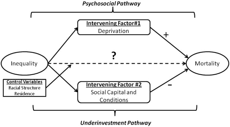
The research framework of this study is presented in Figure 1. Inequality is theorized to be associated with mortality via the psychosocial and underinvestment pathways. Thus, the inequality-mortality relationship may be fully explained by social capital and deprivation as intervening factors, which has not been previously investigated for US counties. Following this framework, the goal of this study is to test the following hypotheses through analysis of US county-level data: (1) Without any other independent covariates, inequality is positively related to mortality, (2) including control variables into the analysis will not fully explain the inequality-mortality relationship, and (3) after controlling for deprivation, social capital, and other variables in the analysis, inequality is not associated with mortality (dashed line). To obtain unbiased estimates and thereby address methodological weaknesses (e.g., spatial dependence) in the literature, this study will take a spatial approach.

Figure 1. Research framework of this study.

3. Methodology and Data

Studies of human mortality are often conducted at the ecological level, in which mortality rates for places are related to other place characteristics. A problem with this approach is that a lack of independence between spatial units may bias analytic results (Cressie, 1993). That is, things like political values, industrial structure, and race/ethnic composition will be more similar among areas that are geographically proximate rather than dispersed (Tobler, 1970). While techniques have been developed to handle spatial dependence, they are underutilized in demographic research (Voss, 2007).

3.1. Spatial analysis approaches

We use both exploratory spatial data analysis (ESDA) and advanced explanatory spatial modeling in this study. The goals of ESDA are to examine whether spatial dependence exists in the data, to determine whether the advanced spatial modeling is necessary, and to assess if the advanced spatial modeling improves the analytic results by accounting for spatial dependence (Cressie, 1993). To achieve these goals, ESDA embraces several techniques, including data visualization, spatial dependence testing, and spatial clusters detection. These methods help researchers to prepare their data for advanced spatial modeling.

Moran's I is commonly used to evaluate whether or not the spatial distribution of data is random. The value of Moran's I is not limited between -1 and 1 and depends on the spatial structure that defines connectivity among spatial units. Moran's I has an expected value close to zero and a positive Moran's I suggests positive spatial dependence, meaning that nearby areas share similar characteristics; negative values indicate that neighboring areas are dissimilar. A detailed discussion of Moran's I can be found elsewhere (Li, Calder, & Cressie, 2007). We also used the local indicator of spatial association (LISA) to identify four local spatial clusters (Anselin, 1995). The high-high and low-low clusters reflect positive spatial dependence and the high-low and low-high clusters represent negative spatial dependence.

With respect to advanced explanatory spatial modeling, this study used the intrinsically conditional autoregressive (CAR) model to test the research hypotheses:

$$Y_i={\beta }_0+{\sum }_{k=1}^K{\beta }_k{x}_{ik}+w_i+h_i,\mathit{\text{where}}{h}_i\sim N(0,1/{\tau }_m).$$ (1)

This model can also be expressed as:

$$Y_i\sim N({\mu }_i,1/{\tau }_m)$$

$${\mu }_i={\beta }_0+{\sum }_{k=1}^K{\beta }_k{x}_{ik}+w_i,$$

where Y_i is the mortality of the ith county and β₀ is the average mortality after accounting for other independent variables and β_k represents the estimated association of covariate x_k with mortality. The distribution of mortality, Y_i, is assumed to follow a normal distribution with a mean μ_i, which is a function of β₀ and β_k. τ_m is a precision parameter for the random error h_i and the reciprocal of τ_m can be regarded as the variance of a normal distribution. In addition to the random error (h_i), the spatially structured errors (w_i) were designated such that the conditional distribution of w_i given other locations w__i that are defined as neighbors can be expressed as equation (2):

$$w_i|w_{-i}\sim N({\sum }_{j\sim i}{w}_j/n_i,1/n_i{\tau }_w),$$ (2)

whereτ_w is the precision parameter for spatial errors, j ∼ i denotes county j is a neighbor of the ith county, and n_i is the total number of neighbors of the ith county. That is, conditioned on the values at the other locations, w_i is assumed to have a mean equal to the mean of its neighbors and a variance that is a function of the number of neighbors. This specification and equation (2) has been commonly used in the CAR model (Besag, York, & Mollié, 1991). The spatially structured errors capture the processes related to the covariates that are not included in a regression model. The first-order queen contiguity approach was used to define the neighbors. In other words, those counties that share a common boundary or a vertex are defined as neighbors. While there is an ongoing debate on whether spatial regression modeling results are sensitive to the choice of the neighboring matrix (Bell & Bockstael, 2000; LeSage & Pace, 2010), this issue is beyond the scope of this study and the common practice should remain valid as long as spatial regression models are correctly specified and estimated.

Note that in equation (1), excluding w_i will make the model a traditional non-spatial regression model with independent homogeneity errors, h_i. As the dependent variable (mortality) is assumed to follow a normal distribution, the independent random errors are assumed to be normally distributed. Therefore, it is preferred to estimate the spatially structured errors only when conducting the advanced spatial modeling (Banerjee, Carlin, & Gelfand, 2004). Both the CAR and non-spatial models were implemented with Markov chain Monte Carlo (MCMC) methods based on the Gibbs sampling algorithm in WinBUGS to generate the posterior distributions of the parameter estimates, β₀ and β_k (Lunn, Thomas, Best, & Spiegelhalter, 2000; Spiegelhalter, Thomas, Best, & Hilks, 1996). Following convention in the Bayesian spatial analysis approach (Thomas, Best, Lunn, Arnold, & Spiegelhalter, 2004), the results will be summarized into the mean values, 95 percent credible regions of the posterior distributions, Monte Carlo errors (MCE), and standard deviations.

We followed the conventional specifications in Bayesian modeling to set up the priors (Banerjee et al, 2004; Thomas et al., 2004). The intercept was assigned a uniform distribution and other parameters were specified with a normal distribution As for the priors on the precision parameters, τ_m and τ_w, a Gamma distribution was assigned. Our model specifications offer so-called vague or weakly informative priors, which minimizes the potential bias introduced by the sampling method. The full Bayesian hierarchical model can be expressed as follows and the WinBUGS code showing the details (e.g., values for mean and precisions) of our spatial model can be found in Appendix 1:

$$[\mathit{\beta },\mathit{w},{\tau }_m,{\tau }_w|\mathit{Y}]\alpha {\mathrm{\Pi }}_{i=1}^{n}N(Y_i|{\beta }_0+{\sum }_{k=1}^K{\beta }_k{x}_{ik}+w_i,1/{\tau }_m)\times \mathit{\text{CAR}}(w|1/{\tau }_w)\times {\mathrm{\Pi }}_{k=1}^{K}N({\beta }_k|0,100000)\times \mathit{\text{Gamma}}({\tau }_m|10,1000)\times \mathit{\text{Gamma}}({\tau }_w|10,1000)$$ (3)

In order to assess the value added by the spatial modeling, the results from the CAR model will be compared with those from the non-spatial model. The Deviance Information Criterion (DIC) will be used for model selections. Similar to the Akaike Information Criterion (Akaike, 1974), smaller values for the DIC indicate a better fit to the data (Spiegelhalter, Best, Carlin, & Van Der Linde, 2002). In general, a DIC difference that is greater than 10 between two models suggests that the one with the lower value is preferred (Spiegelhalter et al., 2002). If the difference is less than 5 and the estimates are dissimilar, the results from both models should be reported to avoid misleading conclusions (Spiegelhalter et al., 2002).

3.2. Measures

Mortality

The mortality rates were calculated with the Compressed Mortality Files (CMF) maintained by the National Center for Health Statistics (NCHS). In order to minimize the fluctuations over time, the five-year (2003-2007) average mortality rates were used in the analysis and it was standardized by the 2000 US age-sex population structure (NCHS, 2010).

Income inequality

Several indicators have been developed to measure income inequality (Allison, 1978) and a concern is whether the choice of inequality indicator alters the findings. Kawachi and Kennedy (1997a) investigated the associations between various inequality indicators and human health, and suggested that the negative inequality-health relationship did not vary greatly by the choice of inequality indicator. The well-known Gini coefficient ranges from 0 (total equality; everyone has the same income) to 1 (completely unequal, one person enjoys all the income). The Gini coefficient was employed to measure inequality within a county and calculated with the household income data from the 2005-2009 American Community Survey (ACS) estimates (US Census Bureau, 2010). We use the top-coded category of $200,000 for the maximum income value, recognizing that this inevitable drawback to the publicly available ACS data necessarily means that inequality will be underestimated.

Deprivation

Originally developed for and widely used in health disparity and epidemiological research (Phillimore et al., 1994), we used the Townsend index of material deprivation (Townsend et al., 1988). Measuring who and how many of them may be subject to deprivation, the index is calculated as the sum of the standardized z-scores for 2005-2009 ACS estimates of percent of economically active people unemployed, percent of households with more than one person per room, percent of households without vehicles, and percent of housing units that are renter-occupied. Counties with higher deprivation index values can be regarded as more deprived. Note that while Singh (2003) developed an area deprivation index for the US, the variables included in the Singh index are similar to our socioeconomic variables (below) and hence we decided to use the Townsend index in this study.

Social capital

We followed Putnam's social capital definition in this study. Two variables were created to measure this concept. One is a social capital index developed and employed by Rupasingha and colleagues (2006) and the other is measure of residential stability. The former is a composite score created with principal component analysis (PCA). The variables used in the PCA were obtained from Rupasingha and Goetz (2008), and include the number of associations per 10,000 population, the number of non-profit organizations per 10,000 population, 2000 census mail response rate, and the voting rate for the 2004 presidential election. As the PCA indicated that one component would suffice to capture 50 percent of the variation, these variables were condensed into the social capital index. This index is assumed to capture the opportunities for residents to interact with one another and thereby grow social ties and capital. Residential stability was measured with two ACS variables: the percentage of individuals aged 5 and older who lived at that same address five years prior, and the percentage of housing units occupied by owners. These variables were standardized and then averaged to yield the residential stability in the analysis.

Racial/ethnic composition

The race/ethnicity structure of a county was captured by three variables: the proportion of non-Hispanic Black, the proportion of Hispanics, and the proportion of other non-Hispanic races (excluding non-Hispanic White). These were extracted from the 2005-2009 ACS estimates.

Socioeconomic and metropolitan status

While the concept of deprivation has captured part of the socioeconomic status (SES) in a county, it is important to control for other social conditions that may be associated with mortality (Link & Phelan, 1995). A factor analysis was implemented to create a single SES score with five socioeconomic variables extracted from the 2005-2009 ACS estimates (factor loadings available upon request), including the log of per capita income, percent of population with at least a bachelor's degree, percent of people employed in professional, administrative, and managerial positions, percent of family with annual income higher than $75,000, and individual poverty rate. Almost 70 percent of the variance among them was explained by a sole factor. We use the factor score, with a higher score representing a better SES.

Following the US Office of Management and Budget, we define metro counties as those with a city of 50,000 or more residents or a total urbanized area of 100,000 population or more, plus contiguous counties with strong economic ties as defined by commuting patterns. All other counties are non-metro.

4. Analytic Results

4.1. Descriptive and exploratory data analysis

Table 1 shows both the ESDA results and non-spatial descriptive statistics, including the Moran's I, mean and standard deviation. We briefly discuss the results: First, variance inflation factors (VIFs) were used to examine if multicollinearity is an issue and the finding that all VIFs are smaller than 4 suggests that multicollinearity would not undermine our conclusions. Second, the Moran's I test indicated that spatial dependence was embedded in every covariate. The proportion of Hispanic population had the largest Moran's I (0.806), whereas stability was the least spatially dependent (0.225). The significance tests for Moran's I showed that the data were not randomly distributed across space. The spatial distribution of mortality is visualized in Figure 2 (the LISA map is available upon request). According to Figure 2, the counties with high all-cause mortality rates were concentrated in the southeastern region and those with low mortality rates were in the Upper Great Plains. This spatial distribution pattern of mortality has been found in other research and, indeed, has persisted for the past few decades (J. S. Cossman et al., 2007). The pattern is seen also in a recent report using state-level data (Miniño et al., 2009). The LISA clustering patterns confirms the distribution of mortality was non-random, suggesting that space matters.

Table 1. Spatial and non-spatial descriptive statistics of the variables in this study (N=3,072).

	VIF#	Moran's I†	Minimum	Maximum	Mean	Std. Deviation
Dependent Variable
Mortality	N.A.	0.529***	0.000	19.777	8.885	1.359
Independent Variables
Inequality:
Gini Coefficient	1.359	0.315***	0.202	0.621	0.431	0.037
Racial Composition:
Proportion of African Americans	1.680	0.802***	0.000	0.868	0.087	0.143
Proportion of Hispanic Population	1.306	0.806***	0.000	0.986	0.076	0.129
Proportion of Other Races	1.375	0.397***	0.000	0.910	0.040	0.069
Socioeconomic and Metropolitan Status:
Metropolitan Status (1=Metro, 0= Non-metro)	1.586	0.387***	0.000	1.000	0.345	0.475
SES Scores	2.029	0.538***	-8.731	4.740	0.000	1.000
Deprivation:
Townsend Deprivation Index	3.372	0.419***	-5.118	21.785	-0.301	2.327
Social Capital:
Social Capital Index	1.628	0.626***	-2.814	10.278	0.000	1.000
Residential Stability	1.824	0.225***	-5.561	2.259	0.000	0.883

^#Variance inflation factors (VIF) are used to detect the multicollinearity among the independent variables.

^†The statistical significance of Moran's I is calculated with the permutation method.

^‡The mean value of a binary variable could be interpreted as the proportion of those coded 1.

N.A.: Not applicable.

^***p-value < 0.001

Figure 2. Spatial distribution of county mortality in the US.

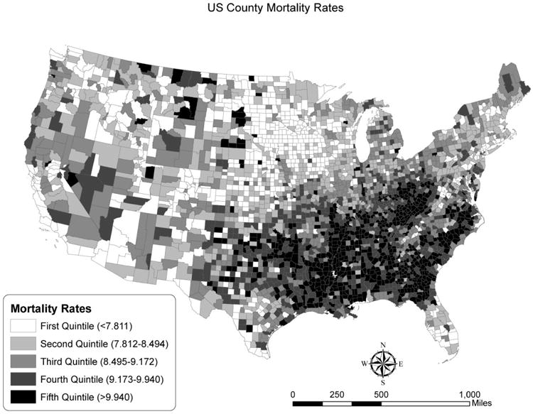
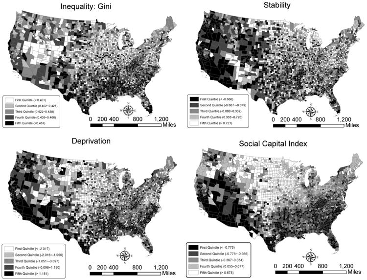
Figure 3 shows the spatial distributions for the key independent variables: inequality, deprivation, the social capital index and residential stability (their LISA maps available upon request). Comparing them with the mortality distribution (Figure 2) can provide clues to how mortality is associated with these variables. For example, counties with high social capital and residential stability are found in the Great Plains, where low mortality rates are observed (note that high social capital and stability are shown with light colors). Similarly, the southeastern counties with high mortality rates are commonly associated with high levels of inequality and deprivation. The comparisons between mortality and the key independent variables provide preliminary support to the hypotheses suggested by the research framework of this study.

Figure 3. Spatial distributions for inequality, deprivation, social capital index and stability.

4.2. Explanatory regression results

To fully examine our hypotheses, three nested models were estimated. Before discussin the results, we would like to emphasize that we did not standardize our independent variables so the interpretations of the coefficients should pertain to the original measurement scales. The fir is a base model that includes only inequality to explain variation in mortality. Model II includes racial composition, SES scores and metropolitan status. The intent here is to confirm the inequality-mortality relationship and to test our second hypothesis. Finally, Model III includes the two variables of key theoretical interest, social capital and deprivation. We estimated these models with both a non-spatial and a Bayesian spatial approach. The results were summarized into Tables 2 and 3, respectively.

Table 2. Non-spatial Bayesian regression results (N=3,072).

	Mean	SD	MCE‡	95% CR#	MCE/SD†
Model I (DIC=10,360)
Constant	4.561	0.271	0.009	(4.019, 5.078)	0.034
Inequality
Gini Coefficient	10.030	0.625	0.021	(8.837, 11.280)	0.034
tau.m (precision parameter for random errors)	0.588	0.015	0.000	(0.559, 0.618)	0.002
Model II (DIC=8,677)
Constant	6.723	0.225	0.006	(6.287, 7.164)	0.025
Inequality
Gini Coefficient	4.036	0.533	0.013	(2.983, 5.065)	0.025
Racial Composition
Proportion of African Americans	2.696	0.145	0.002	(2.415, 2.981)	0.012
Proportion of Hispanic	-1.593	0.142	0.001	(-1.871, -1.317)	0.010
Proportion of Other Races	2.979	0.263	0.002	(2.471, 3.497)	0.009
Socioeconomic and Metropolitan Status
Metropolitan Status	0.551	0.044	0.000	(0.466, 0.636)	0.011
SES Scores	-0.730	0.021	0.000	(-0.772, -0.687)	0.009
tau.m (precision parameter for random errors)	1.017	0.026	0.000	(0.966, 1.068)	0.010
Model III (DIC=8,329)
Constant	7.371	0.235	0.006	(6.905, 7.830)	0.028
Inequality
Gini Coefficient	3.173	0.542	0.015	(2.116, 4.241)	0.027
Racial Composition
Proportion of African Americans	1.970	0.153	0.002	(1.668, 2.268)	0.011
Proportion of Hispanic Population	-2.527	0.151	0.001	(-2.825, -2.239)	0.010
Proportion of Other Races	2.229	0.287	0.003	(1.667, 2.794)	0.010
Socioeconomic and Metropolitan Status
Metropolitan Status	0.227	0.045	0.000	(0.139, 0.314)	0.010
SES Scores	-0.582	0.024	0.000	(-0.630, -0.536)	0.010
Deprivation
Townsend Deprivation Index	0.001	0.013	0.000	(-0.024, 0.027)	0.012
Social Capital
Social Capital Index	-0.384	0.022	0.000	(-0.427, -0.342)	0.009
Residential Stability	-0.106	0.026	0.000	(-0.156, -0.055)	0.009
tau.m (precision parameter for random errors)	1.140	0.029	0.000	(1.083, 1.198)	0.011

^†MCE and SD stand for Monte Carlo errors and standard deviation, respectively.

^‡The values smaller than 0.0005 are shown as 0.000.

^#CR stands for credible region. If the 95% credible region contains 0, the parameter estimate could be concluded to be statistically non-significant.

Table 3. Intrinsically conditional autoregressive (CAR) Bayesian modeling results (N=3,072).

	Mean	SD	MCE‡	95% CR#	MCE/SD†
Model I (DIC=7,421)
Constant	7.612	0.247	0.003	(7.126, 8.092)	0.012
Inequality
Gini Coefficient	2.952	0.573	0.007	(1.841, 4.081)	0.012
tau.m (precision parameter for random errors)	1.560	0.083	0.001	(1.410, 1.740)	0.012
tau.w (precision parameter for spatial errors)	0.791	0.087	0.001	(0.636, 0.978)	0.013
Model II (DIC=6,877)
Constant	7.755	0.216	0.007	(7.328, 8.178)	0.032
Inequality
Gini Coefficient	1.725	0.509	0.016	(0.720, 2.721)	0.032
Racial Composition
Proportion of African Americans	1.546	0.213	0.003	(1.129, 1.960)	0.012
Proportion of Hispanic	0.050	0.239	0.003	(-0.418, 0.528)	0.011
Proportion of Other Races	4.850	0.254	0.003	(4.352, 5.351)	0.010
Socioeconomic and Metropolitan Status
Metropolitan Status	0.160	0.042	0.000	(0.0768, 0.244)	0.011
SES Scores	-0.507	0.023	0.000	(-0.553, -0.460)	0.011
tau.m (precision parameter for random errors)	1.931	0.086	0.001	(1.773, 2.111)	0.010
tau.w (precision parameter for spatial errors)	1.402	0.162	0.002	(1.122, 1.757)	0.010
Model III (DIC=6,765)
Constant	8.214	0.233	0.007	(7.756, 8.669)	0.030
Inequality
Gini Coefficient	1.074	0.528	0.016	(0.044, 2.131)	0.030
Racial Composition
Proportion of African Americans	1.129	0.231	0.003	(0.680, 1.581)	0.012
Proportion of Hispanic	-0.892	0.261	0.003	(-1.413, -0.384)	0.011
Proportion of Other Races	3.842	0.317	0.003	(3.222, 4.463)	0.011
Socioeconomic and Metropolitan Status
Metropolitan Status	0.099	0.042	0.000	(0.017, 0.182)	0.011
SES Scores	-0.468	0.028	0.000	(-0.523, -0.415)	0.011
Deprivation
Townsend Deprivation Index	0.033	0.015	0.000	(0.003, 0.063)	0.013
Social Capital
Social Capital Index	-0.149	0.026	0.000	(-0.201, -0.098)	0.010
Residential Stability	-0.081	0.027	0.000	(-0.135, -0.028)	0.009
tau.m (precision parameter for random errors)	1.909	0.082	0.001	(1.759, 2.081)	0.010
tau.w (precision parameter for spatial errors)	1.614	0.201	0.002	(1.266, 2.051)	0.011

^†MCE and SD stand for Monte Carlo errors and standard deviation, respectively.

^‡The values smaller than 0.0005 are shown as 0.000.

^#CR stands for credible region. If the 95% credible region contains 0, the parameter estimate could be concluded to be statistically non-significant.

Several technical issues need to be addressed before discussing the regression findings. The Monte Carlo errors (MCE) in the tables indicate to what extent the mean of the Monte Carlo samples in our analysis accurately estimates the true posterior mean (Spiegelhalter, Thomas, Best, & Lunn, 2003). A smaller MCE indicates a better sampling process and more accurate estimates. In addition, while it is difficult to determine if a simulation has converged, the trace plots of the sampled values in the analyses demonstrated the ideal patterns (not shown) suggested by Spiegelhalter and colleagues (2003), and the ratios between MCE and standard deviation (MCE/SD in tables) were all smaller than the standard cut point, 0.05. The convergence of these diagnostics suggests that the MCMC sampling process and estimates from the Bayesian explanatory analyses are reliable.

With respect to the empirical findings, without controlling for other covariates inequality was positively associated with mortality (see Model I in Tables 2 and 3). However, the estimated association of inequality with mortality was more than three times larger in the non-spatial (Table 2) than spatial (Table 3) models. More specifically, when the spatial structure is ignored, a one standard deviation increase in the Gini coefficient was related to an increase of (0.037) 37 deaths per 100,000 population in a county. By contrast, the CAR model in Table 3 reduced the number to roughly 11 deaths per 100,000 population. The difference in DIC between the non-spatial and spatial model is 2,939, which suggests that the Model I in Table 3 (spatial approach) fits the data better and should be preferred.

As expected, racial/ethnic composition, SES scores, and metropolitan status only partially account for the inequality-mortality relationship because the parameter estimate for Gini coefficient remained statistically significant in both tables. In addition, the relationships between other independent and the dependent variables follow the expected direction. Notably, both the so-called Hispanic and rural paradoxes are seen. In general, the mortality rate in metro counties is roughly 16 (spatial) to 55 (non-spatial) deaths (per 100,000 population) more than that in non-metro counties. Though including these variables in Model II reduce the inequality-mortality relationship, they do not fully explain why mortality increased with inequality, which leaves room for deprivation and social capital to exert additional explanatory power. It should also be noted that, from Model I to Model II, the magnitude of the association of inequality with mortality shrank almost 60 percent in the non-spatial context, and about 40 percent in Table 3, suggesting that these factors are crucial in understanding the inequality-mortality relationship and that previous findings may overestimate the importance of inequality. As for model fit, while the inclusion of racial/ethnic composition, and socioeconomic and metropolitan status greatly improves the DICs, the CAR model still outperformed the non-spatial model.

Model III included deprivation and social capital, two concepts that are expected to further account for the association between inequality and mortality. Though the estimated effects of the Gini coefficient on mortality were further reduced from Model II by more than 20 percent in both the spatial and non-spatial models, the 95% credible regions did not provide evidence to support the third hypothesis of this study. Specifically, the non-spatial modeling results suggested that the magnitude of the association between inequality and mortality was between 2.12 and 4.24, whereas the CAR model offered an interval between 0.04 and 2.13. Translating these figures into mortality, a one standard deviation increase in Gini coefficient, ceteris paribus, was estimated to forecast an increase of at least 8 deaths per 100,000 population based on the non-spatial modeling. However, when the spatial structure was included, the mortality increase was only 0.16 per 100,000 population. It is clear that the spatial regression results were closer to the hypothesis. With the lowest DIC (6,765), Model III with spatially structured errors fit the data best and thus the subsequent findings were drawn from it.

We hypothesized that deprivation and social capital would be positively and negatively correlated with mortality, respectively. The analytic results support these expectations. A one standard deviation increase in the Townsend deprivation index (2.33, see Table 1) was estimated to increase county-level mortality by almost 8 deaths per 100,000 population. Note that the non-spatial regression results did not suggest a significant association of deprivation with mortality, which is the only discrepancy in significant predictors between Tables 2 and 3. One possible explanation may be drawn from the distribution maps of deprivation and mortality. Most of the California counties had high deprivation (see Figure 3) but they also demonstrated relatively low mortality rates (Figure 2), which contradicts the theoretical expectation. With respect to the measures related to social capital, a one unit change in social capital index and residential stability was associated with the change of roughly 15 and 8 deaths per 100,000 population, respectively. Coupled with the decrease in the effect of inequality on mortality from Model II to Model III, these patterns not only echoed the ESDA findings, but also supported the prospect that social capital and deprivation may intervene between inequality and mortality.

Other control variables were found to be significantly associated with mortality in expected ways. Specifically, the Hispanic Paradox (Abraido-Lanza et al., 1999) was reflected in the negative relationship between the prevalence of Hispanics and mortality, while the concentration of other minority groups was adversely correlated with mortality. Consistent with other research (Yang et al., 2011), a metro disadvantage is seen, such that mortality in metropolitan counties was almost 10 deaths per 100,000 more than that in non-metropolitan counties. Finally, counties with higher SES scores demonstrated lower mortality, and this relationship was independent of deprivation and other social conditions as other studies found (R. E. Cossman, Cossman, Cosby, & Reavis, 2008; McLaughlin et al., 2007). Lynch and colleagues (2004; 2004) have criticized the psychological pathway for ignoring the material environment. The significant relationships of deprivation and SES with mortality found in this study lend credence to this criticism. It should be noted that the models in Tables 2 and 3 had been implemented with standardized covariates (except metropolitan status, SES score, and the Social Capital Index) and the findings did not change (available upon request), suggesting that our MCMC results are reliable.

4.3. Comparing the spatial and non-spatial regression results

Though the DIC suggests that spatial modeling improves model fit greatly, we further applied the ESDA techniques to the random errors (h_i) to better understand the effectiveness of the spatial modeling approach. The results, including visualizatioin, indicated that h_i remains spatially clustered (Moran's I = 0.23) in the non-spatial models and this spatial dependence is subsequently resolved by the CAR model (Moran's I = 0.07) (available upon request).

The spatially structured errors (w_i) capture the underlying spatial processes that lead to the observed mortality pattern but were not considered in the model. Figure 4a shows the geographic distribution of w_i It is apparent that the positive spatial errors are concentrated in the South, particularly Kentucky, Tennessee, Alabama, and Georgia, and gradually decrease with the increase in the distance to theses states. The negative spatial errors were found in southern Florida, southern California, the Four Corners states, Minnesota, Iowa, North and South Dakota. Note that this geographic pattern of w_i is obtained after taking all other covariates into account, and may inform future efforts to understand geographic mortality differentials across the US.

Figure 4. Spatial distribution of the spatially structured errors and the predicted results.

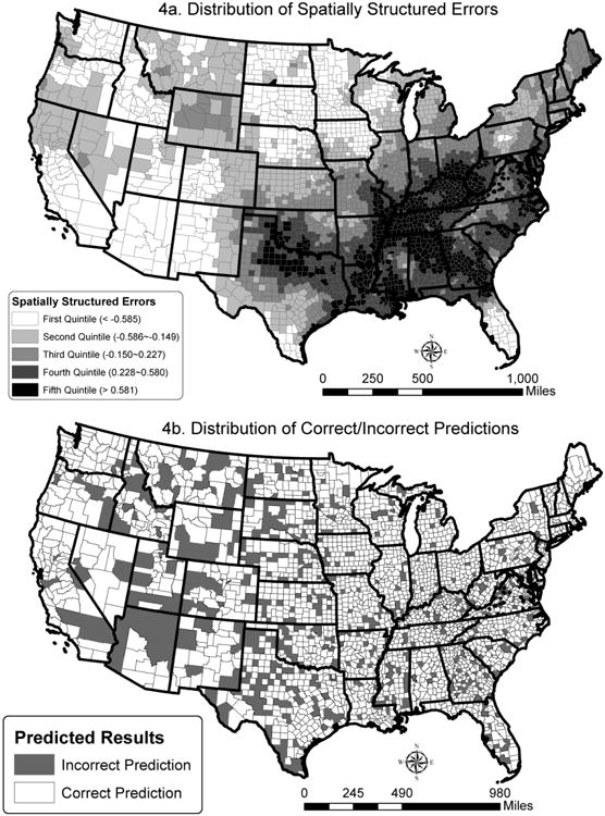
Finally, the Bayesian approach provided the 95 percent credible region for the estimated mortality rate for each county. Should more observed mortality rates (from CMF) fall into the credible regions, the model's ability to predict would be better. Note that whereas the non-spatial model could only capture less than 10 percent of the counties in the contiguous US (286 counties), the CAR model improved the successful prediction to over 80 percent (2,492 counties). Figure 4b depicts which counties were correctly predicted (observed mortality falls within the credible region) and which ones were not. We found that the successful rate was the lowest (roughly 75 percent) among the counties with a w_i in the first quintile (see Figure 4a) and the highest (over 86 percent) among those having a w_i in the fourth quintile. Our spatial model specifications seem to fit the counties with positive spatial errors (and high mortality) better than those with negative spatial errors (and low mortality).

5. Discussion and Conclusions

Recent decades have witnessed a well-chronicled increase in income inequality in the US (Burkhauser, Feng, Jenkins, & Larrimore, 2011), which has given rise to concerns about the decline of the American middle class (Frank, 2013), and what this all means for eking out a living at the bottom of the economic hierarchy (Gilbert, 2014). While the placement of individuals and families in this hierarchy is critically important, researchers also have turned their attention to the implications of variation in inequality at an ecological level. In this paper we have focused on the most fundamental indicator of human well-being, mortality, and how it co-varies by income inequality at the county level. We sought to contribute to the literature in this area in two fundamental ways. The first was by taking a decidedly spatial perspective and employing ESDA, spatial regression modeling and a Bayesian approach to better handle problems of spatial autocorrelation inherent to ecological data. The second was by advancing and - to the extent possible - operationalizing a conceptual model that links inequality and mortality through a psychosocial pathway (via deprivation) and an underinvestment pathway (via social capital).

Analyzing county-level data from the National Center for Health Statistics, the U.S. Census Bureau and other sources for the mid-2000's, we found a positive and significant association between income inequality and mortality that was partially explained by racial composition, SES scores and metropolitan status, thus confirming our first two hypotheses. We further documented that the inequality-mortality association attenuated still more (by more than 20 percent) when controlling for social capital and deprivation, each of which impacted mortality in the expected direction. However, the Gini coefficient remained a significant correlate of mortality and thus our third hypothesis was not supported. Other unmeasured mechanisms between inequality and mortality must be operating and/or the measures of social capital and deprivation may be imperfect.

Our findings suggest the need for future theoretical consideration and empirical investigation of how inequality gets under the skin. It is plausible that counties with high inequality area also marked by the spatial segregation of high- and low-income groups – that income inequality is positively associated with income segregation (Reardon & Bischoff, 2011). Neighborhoods and residential areas where low-income households are found might then suffer from healthcare, educational, and other location disadvantages (Reardon & Bischoff, 2011) that compromise local population health. As noted earlier, if those in better off neighborhoods are availing themselves of higher quality services elsewhere, they may be disinclined to invest in infrastructures closer to home, exacerbating the intro-county association between inequality and health. Moreover, drawing on notions of environment justice, income segregation might well manifest in the disproportionate exposure to environmental hazards or other risk factors that increase the risk of disease and mortality (Brulle & Pellow, 2006). Future work with the right sub-county data can explore these possibilities. Similarly, we also lack direct measurement of the psychological stresses thought to correlate with income inequality – stresses that particularly affect those at the bottom of the economic hierarchy and that would compromise health. Our analysis indicates that income inequality is positively associated with mortality and confirms some of the reasons why. A full accounting will need to consider these and other mechanisms that may be operating at the sub-county level.

Several limitations and caveats deserve mention. First, the data are cross-sectional and the results should not be construed as necessarily causal in nature. Longitudinal data for all the variables would better afford an assessment of causality. Second, this study examined all-cause mortality in the contiguous US counties. The findings cannot be generalized to other aggregate levels, such as Census tracts. That said, this study is subject to the modifiable areal unit problem (MAUP) (Fotheringham & Wong, 1991; Openshaw, 1983) which cautions that analyses at alternative levels of aggregation may yield different results. As there is no solution to MAUP, this limitation is shared by all published ecological studies of this sort. Third, it has been argued that inequality is a multi-dimensional concept and income inequality used in this study is only one aspect of it (Deaton, 2003). Future work should be extended to explore whether other dimensions of inequality – for example in wealth, power, or prestige – are associated with mortality. Fourth, a related problem is that the Gini Index or other singular indicators of inequality within places can mask spatial differences in underlying income distributions. For example, the same middling degree of inequality could prevail in a place where the spread is largely between middle- and high-income groups, and in another locale where the spread is between the poor and those in the middle. To a degree we contend empirically with this problem in our analysis by controlling for SES. However, future work should consider using decomposable measures of inequality (e.g., Theil's (1967) entropy index) to assess how whether and how different types of inequality are related to mortality, particularly with a spatial perspective. Finally, given the fact that this is an ecological study, the perception of relative deprivation, migration history, and other individual-level attributes are unknown. Using a multilevel analytic perspective to examine our research framework is necessary in the future.

Some policy implications likewise suggest themselves here. First, even after controlling for deprivation and social capital, income inequality remains a determinant of mortality. To directly address this association, more progressive tax structures or other transfer mechanisms would not only reduce income inequality, but could generate additional resources to be invested in disadvantaged areas. Second, since the Townsend index measures who and how many of them may be subject to relative deprivation, our finding suggests that providing timely employment information, reducing employment mismatch, ameliorating overcrowding living condition, and ensuring the access to the public transportation may help to counterbalance the adverse impact of deprivation on mortality. Third, to enhance the beneficial effect of social capital on mortality, it may be helpful to encourage participation in non-profit organizations or sports clubs and to create opportunities for residents to establish a strong social network. Via these groups and activities, residents may be more engaged in local communities and more willing to help one another, eventually improving population health. Finally, somewhat related to overcrowding in deprivation, promoting affordable housing may engender a stable community where social capital can be developed and population health can be further advanced.

References

- Abraido-Lanza AF, Dohrenwend BP, Ng-Mak DS, Turner JB. The Latino mortality paradox: a test of the “salmon bias” and healthy migrant hypotheses. American journal of public health. 1999;89(10):1543–1548. doi: 10.2105/ajph.89.10.1543. [DOI] [PMC free article] [PubMed] [Google Scholar]
- Akaike H. A new look at the statistical model identification. Automatic Control, IEEE Transactions on. 1974;19(6):716–723. [Google Scholar]
- Allison PD. Measures of inequality. American Sociological Review. 1978;43(6):865–880. [Google Scholar]
- Anselin L. Local indicators of spatial association—LISA. Geographical analysis. 1995;27(2):93–115. [Google Scholar]
- Banerjee S, Carlin BP, Gelfand AE. Hierarchical modeling and analysis for spatial data. Chapman & Hall; 2004. [Google Scholar]
- Bartley M, Blane D. Commentary: Appropriateness of deprivation indices must be ensured. BMJ. 1994;309(6967):1479. doi: 10.1136/bmj.309.6967.1479. [DOI] [PMC free article] [PubMed] [Google Scholar]
- Bell KP, Bockstael NE. Applying the Generalized-Moments Estimation Approach to Spatial Problems Involving Micro-Level Data. Review of Economics and Statistics. 2000;82(1):72–82. doi: 10.1162/003465300558641. [DOI] [Google Scholar]
- Besag J, York J, Mollié A. Bayesian image restoration, with two applications in spatial statistics. Annals of the Institute of Statistical Mathematics. 1991;43(1):1–20. [Google Scholar]
- Brulle RJ, Pellow DN. Environmental justice: human health and environmental inequalities. Annu Rev Public Health. 2006;27:103–124. doi: 10.1146/annurev.publhealth.27.021405.102124. [DOI] [PubMed] [Google Scholar]
- Buckingham K, Freeman PR. Sociodemographic and morbidity indicators of need in relation to the use of community health services: observational study. BMJ. 1997;315(7114):994. doi: 10.1136/bmj.315.7114.994. [DOI] [PMC free article] [PubMed] [Google Scholar]
- Burkhauser RV, Feng S, Jenkins SP, Larrimore J. Estimating trends in US income inequality using the Current Population Survey: the importance of controlling for censoring. The Journal of Economic Inequality. 2011;9(3):393–415. [Google Scholar]
- Carstairs V, Morris R. Deprivation and mortality: an alternative to social class? Journal of Public Health. 1989;11(3):210. doi: 10.1093/oxfordjournals.pubmed.a042469. [DOI] [PubMed] [Google Scholar]
- Cossman JS, Cossman RE, James WL, Campbell CR, Blanchard TC, Cosby AG. Persistent clusters of mortality in the United States. American journal of public health. 2007;97(12):2148. doi: 10.2105/AJPH.2006.093112. [DOI] [PMC free article] [PubMed] [Google Scholar]
- Cossman RE, Cossman JS, Cosby AG, Reavis RM. Reconsidering the rural–urban continuum in rural health research: a test of stable relationships using mortality as a health measure. Population Research and Policy Review. 2008;27(4):459–476. [Google Scholar]
- Cressie NAC. Statistics for spatial data. John Willey & Sons; 1993. [Google Scholar]
- Daly MC, Duncan GJ, Kaplan GA, Lynch JW. Macro to micro links in the relation between income inequality and mortality. Milbank Quarterly. 1998;76(3):315–339. doi: 10.1111/1468-0009.00094. [DOI] [PMC free article] [PubMed] [Google Scholar]
- Deaton A. Relative deprivation, inequality, and mortality. National Bureau of Economic Research Cambridge; Mass, USA: 2001. [Google Scholar]
- Deaton A. Health, inequality, and economic development. Journal of Economic Literature. 2003;41:113–158. [Google Scholar]
- Deaton A, Lubotsky D. Mortality, inequality and race in American cities and states. Social Science & Medicine. 2003;56(6):1139–1153. doi: 10.1016/s0277-9536(02)00115-6. [DOI] [PubMed] [Google Scholar]
- Fotheringham AS, Wong D. The modifiable areal unit problem in multivariate statistical analysis. Environment and Planning A. 1991;23(7):1025–1044. [Google Scholar]
- Frank R. Falling behind: How rising inequality harms the middle class. Vol. 4. Univ of California Press; 2013. [Google Scholar]
- Gilbert D. The American class structure in an age of growing inequality. Sage; 2014. [Google Scholar]
- Haining RP. Spatial data analysis: theory and practice. Cambridge Univ Pr; 2003. [Google Scholar]
- Kaplan GA, Pamuk ER, Lynch JW, Cohen RD, Balfour JL. Inequality in income and mortality in the United States: analysis of mortality and potential pathways. BMJ. 1996;312(7037):999–1003. doi: 10.1136/bmj.312.7037.999. [DOI] [PMC free article] [PubMed] [Google Scholar]
- Kawachi I, Berkman LF. Social ties and mental health. Journal of Urban Health. 2001;78(3):458–467. doi: 10.1093/jurban/78.3.458. [DOI] [PMC free article] [PubMed] [Google Scholar]
- Kawachi I, Kennedy BP. The relationship of income inequality to mortality: Does the choice of indicator matter? Social Science & Medicine. 1997a;45(7):1121–1127. doi: 10.1016/s0277-9536(97)00044-0. [DOI] [PubMed] [Google Scholar]
- Kawachi I, Kennedy BP. Socioeconomic determinants of health : Health and social cohesion: why care about income inequality? BMJ. 1997b;314(7086):1037. doi: 10.1136/bmj.314.7086.1037. [DOI] [PMC free article] [PubMed] [Google Scholar]
- Kawachi I, Kennedy BP, Glass R. Social capital and self-rated health: a contextual analysis. American journal of public health. 1999;89(8):1187. doi: 10.2105/ajph.89.8.1187. [DOI] [PMC free article] [PubMed] [Google Scholar]
- Kawachi I, Kennedy BP, Lochner K, Prothrow-Stith D. Social capital, income inequality, and mortality. American journal of public health. 1997;87(9):1491–1498. doi: 10.2105/ajph.87.9.1491. [DOI] [PMC free article] [PubMed] [Google Scholar]
- Kawachi I, Subramanian SV, Kim D. Social Capital and Health. Springer; New York: 2008. pp. 1–26. [Google Scholar]
- LeSage J, Pace RK. The biggest myth in spatial econometrics. 2010 Available at SSRN 1725503. [Google Scholar]
- Li H, Calder CA, Cressie N. Beyond Moran's I: Testing for Spatial Dependence Based on the Spatial Autoregressive Model. Geographical analysis. 2007;39(4):357–375. doi: 10.1111/j.1538-4632.2007.00708.x. [DOI] [Google Scholar]
- Link BG, Phelan J. Social conditions as fundamental causes of disease. Journal of health and social behavior. 1995;35:80–94. [PubMed] [Google Scholar]
- Lobao LM, Hooks G, Tickamyer AR. The sociology of spatial inequality. SUNY Press; 2007. [Google Scholar]
- Lunn DJ, Thomas A, Best N, Spiegelhalter D. WinBUGS-a Bayesian modeling framework: concepts, structure, and extensibility. Statistics and Computing. 2000;10(4):325–337. [Google Scholar]
- Lynch J, Kaplan GA. Understanding how inequality in the distribution of income affects health. Journal of Health Psychology. 1997;2(3):297–314. doi: 10.1177/135910539700200303. [DOI] [PubMed] [Google Scholar]
- Lynch J, Smith GD, Harper S, Hillemeier M. Is Income Inequality a Determinant of Population Health? Part 2. US National and Regional Trends in Income Inequality and Age and Cause Specific Mortality. Milbank Quarterly. 2004;82(2):355–400. doi: 10.1111/j.0887-378X.2004.00312.x. [DOI] [PMC free article] [PubMed] [Google Scholar]
- Lynch J, Smith GD, Harper S, Hillemeier M, Ross N, Kaplan GA, Wolfson M. Is income inequality a determinant of population health? Part 1. A systematic review. Milbank Quarterly. 2004;82(1):5–99. doi: 10.1111/j.0887-378X.2004.00302.x. [DOI] [PMC free article] [PubMed] [Google Scholar]
- Marmot MG. The status syndrome: How social standing affects our health and longevity. Times Books; 2004. [Google Scholar]
- McLaughlin DK, Stokes CS, Nonoyama A. Residence and income inequality: Effects on mortality among US counties. Rural Sociology. 2001;66(4):579–598. [Google Scholar]
- McLaughlin DK, Stokes CS, Smith PJ, Nonoyama A. Differential mortality across the U.S.: The influence of place-based inequality. In: Lobao Linda M, Hooks Gregory, Tickamyer AR., editors. The sociology of spatial inequality. Albany, NY: SUNY Press; 2007. pp. 141–162. [Google Scholar]
- Miniño AM, Xu J, Kochanek KD, Tejada-Vera B. Death in the United States, 2007. Hyattsville, MD: National Center for Health Statistics; 2009. [PubMed] [Google Scholar]
- NCHS. Compressed Mortality File, 1999-2007 (machine readable data file and documentation, CD-ROM series 20, No2M) Hyattsville, Maryland: National Center for Health Statistics; 2010. [Google Scholar]
- Openshaw S. The Modifiable Areal Unit Problem. Vol. 38. Geo books Norwich; 1983. [Google Scholar]
- Phillimore P, Beattie A, Townsend P. Widening inequality of health in northern England, 1981-91. BMJ. 1994;308(6937):1125. doi: 10.1136/bmj.308.6937.1125. [DOI] [PMC free article] [PubMed] [Google Scholar]
- Putnam RD. Bowling alone: The collapse and revival of American community. Simon and Schuster; 2001. [Google Scholar]
- Reardon SF, Bischoff K. Income Inequality and Income Segregation1. American Journal of Sociology. 2011;116(4):1092–1153. doi: 10.1086/657114. [DOI] [PubMed] [Google Scholar]
- Rey G, Jougla E, Fouillet A, Hémon D. Ecological association between a deprivation index and mortality in France over the period 1997–2001: variations with spatial scale, degree of urbanicity, age, gender and cause of death. BMC public health. 2009;9(1):33. doi: 10.1186/1471-2458-9-33. [DOI] [PMC free article] [PubMed] [Google Scholar]
- Ross NA, Wolfson MC, Dunn JR, Berthelot JM, Kaplan GA, Lynch JW. Relation between income inequality and mortality in Canada and in the United States: cross sectional assessment using census data and vital statistics. BMJ. 2000;320(7239):898. doi: 10.1136/bmj.320.7239.898. [DOI] [PMC free article] [PubMed] [Google Scholar]
- Rupasingha A, Goetz SJ. US County-Level Social Capital Data, 1990-2005. 2008 Retrieved 08/17, 2011. [Google Scholar]
- Rupasingha A, Goetz SJ, Freshwater D. The production of social capital in US counties. Journal of Socio-Economics. 2006;35(1):83–101. [Google Scholar]
- Singh GK. Area deprivation and widening inequalities in US mortality, 1969-1998. American journal of public health. 2003;93(7):1137–1143. doi: 10.2105/ajph.93.7.1137. [DOI] [PMC free article] [PubMed] [Google Scholar]
- Singh GK, Siahpush M. Widening socioeconomic inequalities in US life expectancy, 1980–2000. International Journal of Epidemiology. 2006;35(4):969. doi: 10.1093/ije/dyl083. [DOI] [PubMed] [Google Scholar]
- Song L, Son J, Lin N. Social Capital and Health. In: Cockerham WC, editor. The New Blackwell Companion to Medical Sociology. Malden, MA: Blackwell; 2010. pp. 184–210. [Google Scholar]
- Sparks PJ, Sparks CS. An application of spatially autoregressive models to the study of US county mortality rates. Population, Space and Place. 2010;16:465–481. [Google Scholar]
- Spiegelhalter DJ, Best NG, Carlin BP, Van Der Linde A. Bayesian measures of model complexity and fit. Journal of the Royal Statistical Society Series B, Statistical Methodology. 2002:583–639. [Google Scholar]
- Spiegelhalter DJ, Thomas A, Best NG, Hilks WR. BUGS: Bayesian inference Using Gibbs Sampling, Version 0.5, (version ii) 1996 [Google Scholar]
- Spiegelhalter DJ, Thomas A, Best NG, Lunn D. WinBUGS user manual. Vol. 2 MRC Biostatistics Unit; Cambridge, UK: 2003. [Google Scholar]
- Taylor RB. Neighborhood responses to disorder and local attachments: The systemic model of attachment, social disorganization, and neighborhood use value. Paper presented at the Sociological Forum 1996 [Google Scholar]
- Theil H. Economics and information theory. Amsterdam: North Holland; 1967. [Google Scholar]
- Thomas A, Best NG, Lunn D, Arnold R, Spiegelhalter DJ. GeoBugs user manual. Cambridge: Medical Research Council Biostatistics Unit; 2004. [Google Scholar]
- Tobler WR. A computer movie simulating urban growth in the Detroit region. Economic Geography. 1970;46:234–240. [Google Scholar]
- Townsend P, Phillimore P, Beattie A. Health and deprivation: inequality and the North. Routledge Kegan & Paul; 1988. [Google Scholar]
- US Census Bureau. American Community Survey 2005-2009 5-year Estimates. Washington, DC: 2010. [Google Scholar]
- Voss PR. Demography as a spatial social science. Population Research and Policy Review. 2007;26(5):457–476. [Google Scholar]
- Voss PR, Long DD, Hammer RB, Friedman S. County child poverty rates in the US: a spatial regression approach. Population Research and Policy Review. 2006;25(4):369–391. [Google Scholar]
- Wilkinson RG. The impact of inequality. Social Research: An International Quarterly. 2006;73(2):711–732. [Google Scholar]
- Wilkinson RG, Pickett KE. Income inequality and population health: a review and explanation of the evidence. Social Science & Medicine. 2006;62(7):1768–1784. doi: 10.1016/j.socscimed.2005.08.036. [DOI] [PubMed] [Google Scholar]
- Wilkinson RG, Pickett KE. The spirit level: why equality is better for everyone. Penguin; 2009. [Google Scholar]
- Williams DR, Mohammed SA, Leavell J, Collins C. Race, socioeconomic status, and health: Complexities, ongoing challenges, and research opportunities. Annals of the New York Academy of Sciences. 2010;1186(1):69–101. doi: 10.1111/j.1749-6632.2009.05339.x. [DOI] [PMC free article] [PubMed] [Google Scholar]
- Yang TC, Jensen L, Haran M. Social capital and human mortality: explaining the rural paradox with county-level mortality data. Rural Sociology. 2011;76(3):347–374. doi: 10.1111/j.1549-0831.2011.00055.x. [DOI] [PMC free article] [PubMed] [Google Scholar]
- Yang TC, Teng HW, Haran M. The impacts of social capital on infant mortality in the US: a spatial investigation. Applied Spatial Analysis and Policy. 2009;2(3):211–227. [Google Scholar]