RETROSPECTIVE DETECTION OF INTERLEAVED SLICE ACQUISITION PARAMETERS FROM FMRI DATA

Abstract

To minimize slice excitation leakage to adjacent slices, interleaved slice acquisition is nowadays performed regularly in fMRI scanners. In interleaved slice acquisition, the number of slices skipped between two consecutive slice acquisitions is often referred to as the ‘interleave parameter’; the loss of this parameter can be catastrophic for the analysis of fMRI data. In this article we present a method to retrospectively detect the interleave parameter and the axis in which it is applied. Our method relies on the smoothness of the temporal-distance correlation function, which becomes disrupted along the axis on which interleaved slice acquisition is applied. We examined this method on simulated and real data in the presence of fMRI artifacts such as physiological noise, motion, etc. We also examined the reliability of this method in detecting different types of interleave parameters and demonstrated an accuracy of about 94% in more than 1000 real fMRI scans.

1. Introduction

Functional Magnetic Resonance Imaging (fMRI) scan is a 4-dimensional image composed of repetitive acquisitions of 3-dimentional brain images. Echo Planner Imaging (EPI), a fast acquisition sequence which makes fMRI possible, does not capture the complete 3D brain volume in single snapshot. Instead, multiple 2D slices are acquired sequentially and stacked to create a 3D brain image. During slice excitation, adjacent slices often get partially excited as well. This is due to the inhomogeneity of the magnetic field, as well as the non-linearity in the electronics generating the slice excitation RF pulse. This leakage of the excitation to adjacent slices causes a profound distortion to the EPI scans. To suppress the destructive effects of the excitation leakage, interleaved slice acquisition has been used regularly in almost all fMRI scanners. The order in which interleaved slices are acquired might be different across manufacturers and developed pulse sequences. For instance, while many scanners utilize even-odd interleaved acquisition, Philips scanners often use $\mathit{\text{round}}(\sqrt[2]{\mathit{\text{SliceNumber}}})$ as their interleave parameter. This means, for example, that a brain image with 37 slices is acquired in the order of every 6^th slice. In other words, the interleave parameter becomes dependent on the number of slices, which allows it to vary from image to image even when acquired with the same scanner.

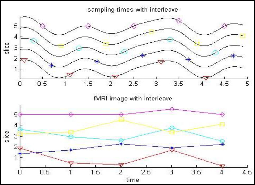
Interleaved slice acquisition is not without consequence: voxels that are spatially adjacent in the acquisition axis are no longer recorded at temporally contiguous times. Indeed, as seen in Fig. 1, voxels’ signals in a small area normally representing a common hemodynamic response may appear totally different after interleaved slice acquisition. Any processing step that requires operations for voxels that expand over more than one slice will be problematic, if the timings of the voxels in each slice are not corrected according to the time of their acquisitions. Many slice timing correction algorithms were proposed to synchronize the sampling time of all the voxels in an image using different interpolation types [1], [2].

Fig. 1.

Illustration of the effect of interleaved slice acquisition

To correct for interleaved slice timing acquisition, the interleaved slice order (interleave parameter) is required. Without this parameter, it is impossible to perform slice timing correction. A recent study shows the undesirable effects of skipping slice timing correction [3]. Most fMRI software packages (SPM, AFNI, or FSL) have preprocessing sub-routines specifically designed for slice timing correction; however, they all require knowledge of the interleave parameter. This parameter should be stored in the fMRI file’s header during data acquisition. However, it is surprising how often such an important parameter is missing from the fMRI file’s header. Currently, no methods exist to retrospectively detect the interleave parameter from the fMRI data itself. This issue has become more pressing with the recent demands for sharing fMRI data collected with NIH/NSF funds. Sharing data without this parameter, as it is done in one of the largest online resting-state fMRI datasets (fcon_1000 [4]), reduces the validity of the results obtained with this data.

We propose in this article a method to retrospectively detect the interleave parameter using only raw fMRI data. The proposed method is based on a temporal-distance correlation function of the fMRI signal along different axes, and its specific characteristic along the axis in which the interleaved slice acquisition is performed. Section II describes a brief theory behind the proposed method. The details of the detection method are given in section III, and its examination on simulated and real fMRI data is given in section IV. We end with discussion and conclusion in section V.

2. Temporal-Distance Correlation

Spatiotemporal fMRI signal, f (s, t), is an inherently smooth but noisy signal (A smooth hemodynamic response with added noise) which is sampled at a rate of 1/TR (TR: repetition time is the duration between two consecutive acquisitions of the same slice). A conventional fMRI signal consists of four dimensions, three spatial Cartesian directions, s = (x, y, z), and one time component t.

This paper focuses on the properties of temporal correlations of the fMRI signal along different axes. Temporal correlation function between two points, s and s′, is given by the following equation,

$$\rho (s,s\prime )=\frac{1}{n}\sum _t\frac{(f(s,t)-\overline{f(s,t)})(f(s\prime ,t)-\overline{f(s\prime ,t)})}{{\sigma }_{f(s,t)}{\sigma }_{f(s\prime ,t)}}$$ (1)

where n is the number of samples in temporal domain, and $\overline{f(․)}$, and σ_f(․) are the temporal mean and standard deviations of signal f(․), respectively. Note that ρ(․, ․) is a six dimensional correlation function, giving a distinct 3 dimensional correlation map for each brain. These correlation maps are already the basis for many resting-state fMRI data analyses. However, in the current method we used them for the purpose of detecting the interleaved slice acquisition parameter.

2.1 Temporal-distance correlation

We define the temporal-distance correlation function of the fMRI signal as the average of all the temporal correlations of voxel pairs that are spatially located in certain distances and directions from each other. In general, a temporal-distance correlation function is a two dimensional function, with one axis indicating the absolute distance, and another giving the direction in which the voxel pairs are located. In its most widespread formulation, it is given by following equation,

$$\xi (\eta ,d)=\frac{1}{m}\sum _{\forall s,s\prime ,|s-s\prime |=\eta \&\measuredangle (s-s\prime )=d}\rho (s,s\prime )$$ (2)

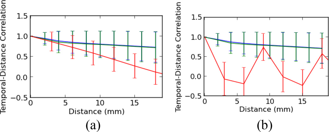
where m is the total number of voxel pairs found in the fMRI data that are located within a distance of η and direction of d. In addition, |s − s′| is the length, and ∡(s − s′) is the angle, of the vector connecting s to s′. In general, d needs to have more than one dimension to cover the entire 3D space of the fMRI volume, but for the purpose of this paper we are only interested in three main directions along Cartesian axes (x, y, z). For instance, ξ(2, z) is the temporal-distance function for all the voxel pairs that are located exactly 2 mm from each other along the Z axis. Typically, as the spatial distance between two points (s, s′) increases, the temporal-distance correlation function monotonically decreases. This simple characteristic of the temporal-distance correlation function should be observed across all three axes, as seen in Fig. 2a. Because data on X/Y plane are acquired instantaneously, they exhibit much less temporal decorrelation than the axis of acquisition (Z), accounting for the steeper slope. However, in the case of interleaved slice acquisition, this decreasing monotonic trend will be disrupted in the slice selected axis, as seen in Fig. 2b, for the interleave parameter of 2 along the Z axis. This disruption is due to the fact that neighboring voxels along Z the axis are not sampled immediately after each other in the interleaved slice acquisition protocols. Based on this simple property of the temporal-distance correlation function, we can recover the interleave parameter from the raw, unprocessed fMRI data. Next, we explain the method that we developed for our detection algorithm.

Fig. 2.

Temporal-distance correlation functions for three main axes (x:blue, y: green, z: red) and for η between 0 to 20 mm for (a) sequential slice acquisition and (b) interleaved slice acquisition using simulated data.

3. Methods

We first preprocess the fMRI data to remove as much noise as possible from the image. To do this, we mask out nonbrain image areas using a series of histogram-based thresholdings.

3.1 Cross-correlogram of slices

Even though the temporal-distance correlation functions monotonically decrease by increasing the distance η, there is a significant amount of variation in the temporal-correlations at each η, as plotted in Fig. 2 with standard deviation bars. There are many reasons behind these variations, such as local neuronal activity, noise, involuntary head motion, and physiological noise. In the real data these variations often cause the detection algorithm to fail. To solve this issue, we propose introducing a one-step dimension reduction before computing the temporal correlations. This also facilitates the implementation of the method and significantly reduces the number of required operations. Dimension reduction is performed on the data by averaging over the plane perpendicular to the acquisition axes. Averaging the signals of all voxels within a slice will reduce the variations of the signals due to factors other than interleaved slice acquisition, while preserving the variation due to slice timing between two adjacent slice signals. For instance, given an fMRI signal f (x, y, z, t), a slice average over the X/Y plane can be obtained as:

$$f_{\mathit{\text{slice}}}(z,t)=\frac{1}{NM}\sum _x\sum _{y}f(x,y,z,t)$$ (3)

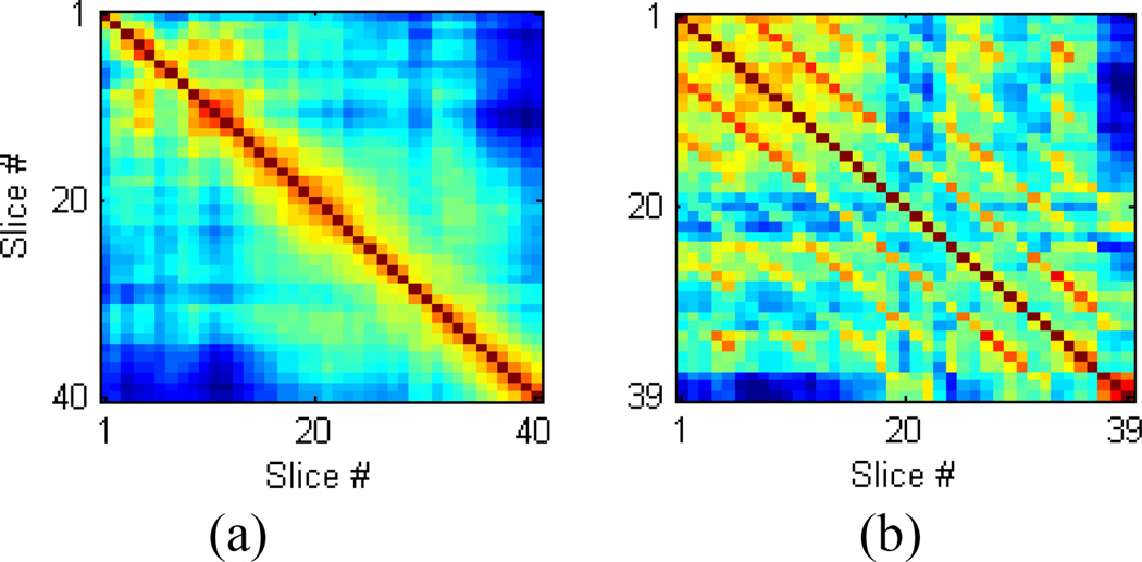
where N and M are the number of voxels in the X and Y-axis, respectively. This is called a slice signal. Equation (3) can be re-formulated for the other two planes (X/Z, Y/Z) as well. In our X/Z averaged signal, each slice along the Z axis has an averaged signal, and their temporal correlation is given by ρ(f_slice (z, t), f_slice (z′, t)). By plotting every possible pairwise correlation of the slice signals, a matrix of correlations can be created (Fig. 3). This matrix is called a cross-correlogram.

Fig. 3.

a) A cross-correlogram of an image with no interleave and b) A cross-correlogram of an image with interleave 6, from real data.

Typically, an fMRI image sampled sequentially (no interleave) will have a correlation pattern similar to the one shown in Fig. 3a. The series of “1’s” along the diagonal axis represent the correlation of a slice compared to itself, which is always the maximum. Moving away from the diagonal axis, we see a generally decreasing function, as we compare slices with more spatial distance.

In an interleaved fMRI image, we would expect slices to have a higher correlation with those slices sampled immediately before or after them, than with slices sampled at some later time. We see this in Fig. 3b. In our analysis, this appears as additional diagonal “stripes” in the cross-correlogram (Fig. 3b). These stripes indicate an increase in the correlation of two spatially separated slices, which is consistent across the entire image. The distance between these stripes is the interleave value.

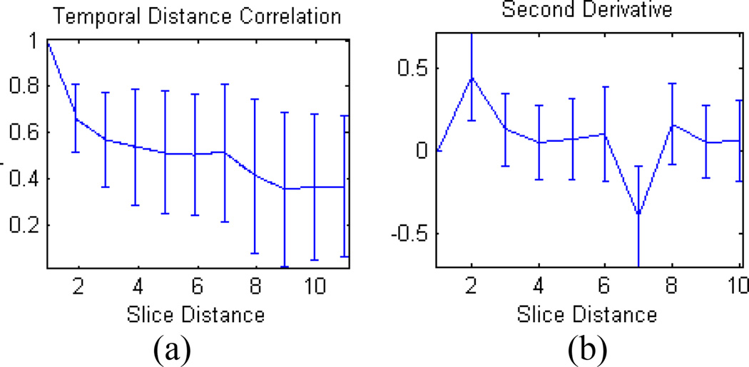
Even after dimension reduction, there are cases where the cross-correlogram is noisy, and not as clear as the one shown in Fig. 3b. Because of this, a simple peak detection algorithm is insufficient to reliably extract the interleave parameter. Instead, the correlation may gradually increase until the interleave slice is reached, at which point it decreases rapidly. We determined through observation that the second derivative of the signal, in those cases, provides a better indicator of where the first interleaved slice is taken. Fig. 4b shows the change in slope as a large drop at slice number 7, whereas the original signal, in Fig. 4a, shows only a slight increase at that slice. Though it is clear from Fig. 4 that the second derivative easily picks out the global maximum, it does not provide any measure of certainty. We address this shortcoming by using statistical inference to provide a measure of certainty in the detected interleave parameter.

Fig 4.

(a) The average of a temporal distance function (b) its second derivative, from a typical real data.

3.2 Statistical Analysis

We perform a simple statistical analysis to detect the most significant minimum from a number of local minima found in the profile of the temporal-distance function’s second derivative, and do the same to the maxima in the original function. Then, using the p-values obtained from the two profiles, we decide which one to use as the final result.

To achieve this, the following steps are taken. All local minima in the second derivative that pass a cutoff threshold are compared against their two neighboring values using a basic student t-test to determine if they are significantly smaller than the two neighbors. Comparison with each neighbor is carried out separately, with statistical t-test giving separated p-values. The geometric mean is used to combine the two significance levels and gives the final p-value for the minimum point. The minimum point with lowest combined p-value is selected as the global minimum for the second derivative. The same process is performed to detect the global maximum of the temporal-distance function and its significance level (combined p-value). Note that the most significant maximum/minimum is not necessarily the same as the global maximum/minimum of the mean signal. If both of the extremes in the temporal-distance function and its second derivative point to the same value, then that value is reported as the interleave parameter with its p-value. Otherwise, the minimum of the second derivative is selected unless its p-value is larger than 10^α times the p-value for global maximum of the temporal-distance function. We biased our decision towards the second derivative, because it often gives more accurate results. We set α = 1.5 in our examination, which gave the most accurate results. However, others might find that different values optimize their process. This statistical analysis gives a certainty measure in extremely noisy and hard-to-detect cases. Low certainty values may require a manual inspection of the data to verify the interleave value. A weak significance value for this analysis is generally 10⁻⁵ or larger, as typical values are 10⁻⁹ or smaller.. Preforming the analysis on multiple images acquired identically and comparing detected interleave values can help increase certainty.

4. Examination Results

4.1 Simulated and real data

We used both simulated and real data to examine the success rate of the detection method proposed in this paper. Using the method described in [3] to generate our simulated data, we generated 10 minutes of scan, with in-plane resolution of 112×112, and 37 slices. The voxel size was set to 2×2×3 mm³ and the TR equal to 2 seconds. A neuronal stimulus sequence containing 20 pulses with random onset (at least 10s apart) and width (5 to 30 second) was independently created for each ROI. The neuronal stimulus sequence convolves with canonical hemodynamic impulse response functions included in SPM to generate the underlying BOLD signal. Subsequently, cardiac (f=1.005 Hz) and respiratory (f=0.25 Hz) noises were added to the signal. To simulate the interleaved slice acquisition, the original high frequency sampled signals (f_s=20 Hz) were subsampled with f_ss=0.5 Hz and with a time-shift (phase) specifically set for each slice according to the interleaved parameter. Ten images were generated with 6 different interleave parameters, from one to six (one indicating no interleave). To simulate the head motion, we displaced each volume of the simulated fMRI data using different transformation matrices. The transformation matrices were obtained from real subjects’ involuntary movements in the scanner using typical realignment algorithms.

Real data were obtained from our group’s on-going studies of task-based and resting-state fMRI data as well as datasets collected outside our group. 56 resting-state and 300 task-based fMRI data with interleave parameters of 6, as well as 205 task-based fMRI with even-odd interleave, were examined. To expand the examination of our method to datasets collected outside our group, we examined 474 randomly selected fMRI images from the fcon_1000 dataset [4], which is available online for public use.

4.2 Results

The developed algorithm detected the interleaved parameter in all 60 simulated images with 100% accuracy. For 356 onsite fMRI data images acquired with an interleaved parameter of 6, the detection accuracy dropped to 91%. For the 200 task-based fMRIs with even-odd interleave, the accuracy was 93%. For the 474 randomly selected restingstate fMRI scans from fcon_1000 dataset, the accuracy was 97%. It is important to note that the fcon_1000 dataset is collected in 23 sites, each with different scanner and acquisition pulse sequence. Only images with cross-correlograms that could be analyzed visually were used.

4.3 Software

Our detection algorithm was developed in Matlab, and it is given public access in our group’s website [5]. This function takes raw fMRI data and gives the direction and interleave parameter with its p-value, which indicates the result’s accuracy. Sufficient amount of comments and guidelines are provided to make the software easily usable by average researchers in the field of neuroimaging.

5. Discussion AND Conclusion

Slice timing correction, as an important pre-processing step of fMRI data, cannot be implemented without interleave parameters. In the case of scrappy fMRI data header files (which is often the case), finding the correct interleave parameter is a nontrivial task- especially for old data shared online with minimal or no explanation. This problem was so difficult that some of the neuroimaging software packages suggested removing this important step from their preprocessing pipeline, despite many studies emphasizing the necessity of slice timing correction [3]. In this article we proposed and developed a technique which retrospectively detects the interleave parameter and the axis in which it is applied, using only fMRI data. We showed successful detection of the parameters on simulated data and a very high success rate on in-house and off-site fMRI data. Our technique is built upon a very simple property of temporal-distance correlation functions in spatiotemporal fMRI signals. In addition, we shared the developed Matlab function on our group webpage for public use [5].

Some fMRI scanners do not start their slice acquisition from slice zero, as we assumed in our technique. Though this is done for reasons unrelated to interleaved slice acquisition, it influences the results of the slice timing correction. Finding the start point can also be beneficial, and can be considered as the next phase of this project.

References

- 1.Henson R, Buechel C, Josephs O, Friston K. The slice-timing problem in event-related fMRI. Neuroimage. 1999;9:125–125. [Google Scholar]
- 2.Calhoun V, Golay X, Pearlson G. Improved fMRI slice timing correction: interpolation errors and wrap around effects Proceedings. ISMRM. 2000:810. [Google Scholar]
- 3.Sladky R, Friston KJ, Tröstl J, Cunnington R, Moser E, Windischberger C. Slice-timing effects and their correction in functional MRI. Neuroimage. 2011 Sep.58(2):588–594. doi: 10.1016/j.neuroimage.2011.06.078. [DOI] [PMC free article] [PubMed] [Google Scholar]
- 4.Biswal BB, et al. Toward discovery science of human brain function. Proc. Natl. Acad. Sci. U. S. A. 2010 Mar.107(10):4734–4739. doi: 10.1073/pnas.0911855107. [DOI] [PMC free article] [PubMed] [Google Scholar]
- 5.Razlighi QR, Parker D. Interleave Detection Software (matlab) Pre Processing Project. 2013 [Online]. Available: http://cumc.columbia.edu/dept/sergievsky/cnd/Zip/InterleaveDetection.zip. [Google Scholar]