The Anatomical and Functional Organization of the Human Visual Pulvinar

Abstract

The pulvinar is the largest nucleus in the primate thalamus and contains extensive, reciprocal connections with visual cortex. Although the anatomical and functional organization of the pulvinar has been extensively studied in old and new world monkeys, little is known about the organization of the human pulvinar. Using high-resolution functional magnetic resonance imaging at 3 T, we identified two visual field maps within the ventral pulvinar, referred to as vPul1 and vPul2. Both maps contain an inversion of contralateral visual space with the upper visual field represented ventrally and the lower visual field represented dorsally. vPul1 and vPul2 border each other at the vertical meridian and share a representation of foveal space with iso-eccentricity lines extending across areal borders. Additional, coarse representations of contralateral visual space were identified within ventral medial and dorsal lateral portions of the pulvinar. Connectivity analyses on functional and diffusion imaging data revealed a strong distinction in thalamocortical connectivity between the dorsal and ventral pulvinar. The two maps in the ventral pulvinar were most strongly connected with early and extrastriate visual areas. Given the shared eccentricity representation and similarity in cortical connectivity, we propose that these two maps form a distinct visual field map cluster and perform related functions. The dorsal pulvinar was most strongly connected with parietal and frontal areas. The functional and anatomical organization observed within the human pulvinar was similar to the organization of the pulvinar in other primate species.

SIGNIFICANCE STATEMENT The anatomical organization and basic response properties of the visual pulvinar have been extensively studied in nonhuman primates. Yet, relatively little is known about the functional and anatomical organization of the human pulvinar. Using neuroimaging, we found multiple representations of visual space within the ventral human pulvinar and extensive topographically organized connectivity with visual cortex. This organization is similar to other nonhuman primates and provides additional support that the general organization of the pulvinar is consistent across the primate phylogenetic tree. These results suggest that the human pulvinar, like other primates, is well positioned to regulate corticocortical communication.

Introduction

The pulvinar is the largest nucleus in the primate thalamus. Across nonhuman primate species, the pulvinar has been traditionally divided into anterior (oral), inferior, lateral, and medial subdivisions based on anatomical properties (Olszewski, 1952), although finer subdivisions have been identified (Gutierrez et al., 1995; Stepniewska and Kaas, 1997; Adams et al., 2000). In nonhuman primates, the pulvinar is heavily interconnected with visual cortex. Generally, cortical areas that are directly connected are also indirectly interconnected via the pulvinar with layer-specific cortical connections forming distinct feedforward and feedback loops. Individual visual areas project to specific parts of the pulvinar (Benevento and Rezak, 1976; Ungerleider et al., 1984; Schmahmann and Pandya, 1990; Adams et al., 2000; Gutierrez et al., 2000; Shipp, 2001). Striate and extrastriate areas project to the lateral and inferior pulvinar. Middle temporal area MT projects to the inferior and medial pulvinar. Parietal and frontal areas project to dorsal portions of the lateral and medial pulvinar. Given this extensive interconnectivity with cortex, the pulvinar is thought to play a fundamental role in regulating corticocortical communication (Jones, 2001; Sherman and Guillery, 2002; Shipp, 2003; Saalmann and Kastner, 2011).

In nonhuman primates, there are two retinotopic maps of contralateral visual space in lateral and inferior subdivisions of the pulvinar (Gattass et al., 1978; Bender, 1981; Li et al., 2013). However, the organization of these visual field maps appears to differ across primate species (Li et al., 2013). In humans, neuroimaging studies have demonstrated contralateral biases (Cotton and Smith, 2007) and some systematic representation of visual space within the ventral pulvinar (Schneider, 2011; DeSimone et al., 2015). However, the exact organization of these representations in the human has yet to be resolved. Further, the relation of visual field maps to cortical connectivity in humans is unknown.

Using neuroimaging, we investigated the visuotopic organization of the human pulvinar and its profile of functional and anatomical connectivity with visual cortex. We identified two visuotopic maps within the ventral pulvinar. Both maps represented contralateral visual space and shared a foveal representation. Additional representations of contralateral visual space were identified within ventral medial and dorsal lateral regions of the pulvinar. These representations add to the number of visual field maps previously reported within the human posterior thalamus and subcortex (Schneider et al., 2004, 2005; DeSimone et al., 2015). Anatomical connectivity was assessed from diffusion tensor imaging data. Functional connectivity was assessed from data collected during task-free states of rest in which subjects were instructed to either maintain central fixation, or keep their eyes closed. Both anatomical and functional connections between individual cortical areas and the pulvinar appeared to be topographically organized. The organization of the human pulvinar was consistent with prior studies in other primate species. Overall, our results provide additional support that the general organization of the pulvinar is consistent across the primate phylogenetic tree.

Materials and Methods

Participants

Nineteen subjects (aged 20–36 years, nine females) participated in the study, which was approved by the Institutional Review Board of Princeton University. All subjects were in good health with no history of psychiatric or neurological disorders and gave their informed written consent. Subjects had normal or corrected-to-normal visual acuity. Each subject participated in at least two of the following experiments: (1) polar angle thalamus mapping, (2) eccentricity thalamus mapping, (3) high-resolution thalamus anatomical imaging, (4) task-free resting-state, and (5) diffusion tensor imaging. In addition, all subjects participated in three experiments to localize cortical visual field maps: (1) polar angle cortical mapping, (2) eccentricity cortical mapping, and (3) memory-guided saccade task.

Visual display

The stimuli were generated on Macintosh G4, G5, and Mac Pro computers (Apple) using MATLAB software (MathWorks) and Psychophysics Toolbox functions (Brainard, 1997; Pelli, 1997). Stimuli were projected from either a Christie LX650 liquid crystal display projector (Christie Digital Systems) or a Hyperion PST-100984 digital light processing projector (Psychology Software Tools) onto a translucent screen located at the end of the Siemens 3T Allegra and Skyra scanner bores, respectively. Subjects viewed the screen at a total path length of ∼60 cm through a mirror attached to the head coil. The screen subtended either 30° × 30° (Allegra, Siemens), or 51° × 30° (Skyra, Siemens) of visual angle. A trigger pulse from the scanner synchronized the onset of stimulus presentation to the beginning of the image acquisition.

Experimental tasks

Visuotopic mapping: polar angle.

Nine subjects participated in a scan session in which polar angle representations were measured in the thalamus. Visual stimuli consisted of a wedge that rotated either clockwise or counterclockwise around a central fixation point that subtended 0.5° of central space (e.g., Arcaro et al., 2009, their supplemental Fig. 1A). The wedge spanned 1°–15° in eccentricity with an arc length of 45° and moved at a rate of 9°/s. The wedge was filled with 1000 white dots (0.1°, 65 cd/m²) that moved either randomly or in a coherent direction at a rate of 7°/s. Subjects were instructed to maintain fixation while covertly attending to the rotating wedge and to detect a change in the direction of the coherently moving dots by pressing a button with their right index finger. Covert attention directed toward the stimulus has been shown to improve mapping (Arcaro et al., 2009; Bressler and Silver, 2010). The change in direction of the coherently moving dots ranged between 75 and 105 arc degrees. The percentage of coherently moving dots was set at 55%, which was determined to yield an accuracy of ∼75% in a separate behavioral testing session. The direction of motion for the coherent dots changed randomly every 3–5 s. Each run consisted of eight cycles of 40 s each and started with a 20 s no stimulus, fixation period, amounting to an overall run length of 340 s. A total of 8–10 runs were collected in a single scan session for each subject.

All 19 subjects participated in a single scan session in which polar angle representations were measured across visual cortex. Visual stimuli consisted of a checkerboard wedge stimulus (for details, see Swisher et al., 2007; Arcaro et al., 2009, 2011; Wang et al., 2014), although the dot motion stimulus is also well suited for cortical mapping (Arcaro et al., 2009). Timing and stimulus size parameters matched that of the thalamus mapping stimulus. A total of 3–5 runs were collected in a scan session for each subject.

Visuotopic mapping: eccentricity.

Five subjects (who participated in the thalamus polar angle mapping) also participated in a scan session in which eccentricity representations were measured in the thalamus. Visual stimuli consisted of an annulus that expanded around a central fixation point that subtended 0.5° of central space. The duty cycle of the annulus was 10% (i.e., any given point on the screen was within the annulus for only 10% of the time). The annulus increased on a linear scale over a period of 40 s in size and rate of expansion between 0° and 15° eccentricity. The end of each cycle included a 10 s no stimulus, fixation period to enable a clear (temporal) separation of responses to foveal and far peripheral stimulation. The ring was filled with 1000 white dots (0.1°, 65 cd/m²) that moved either randomly or in a coherent direction at a rate of 7°/s within the annulus. Subjects were instructed to maintain fixation while covertly attending to the expanding annulus and to detect a change in the direction of the coherently moving dots by pressing a button with their right index finger. The change in direction of the coherently moving dots ranged between 75 and 105 arc degrees. The percentage of coherently moving dots was set at 65%, which was determined to yield an accuracy of ∼75% in a separate behavioral testing session. The direction of motion for the coherent dots changed randomly every 3–5 s. Each run consisted of eight cycles of 50 s each and started with a 20 s no stimulus, fixation period amounting to an overall run length of 420 s. A total of 8–10 runs were collected in a single scan session for each subject.

All 19 subjects participated in a single scan session in which eccentricity representations were measured across visual cortex. Visual stimuli consisted of a checkerboard ring stimulus (for details, see Swisher et al., 2007; Arcaro et al., 2009, 2011; Wang et al., 2014), although the dot motion stimulus is also well suited for cortical mapping (Arcaro et al., 2009). Briefly, the ring stimulus increased on a logarithmic scale, the duty cycle was 12.5°, and there was no blank period at the end of each cycle. A total of 1–3 runs were collected in a scan session for each subject.

Memory-guided saccade task.

All 19 subjects participated in a single scan session in which a memory-guided saccade task was used to localize topographically organized areas in parietal and frontal cortex (Kastner et al., 2007; Konen and Kastner, 2008a, b). This task incorporates covert shifts of attention, spatial working memory, and saccadic eye movements in a traveling wave paradigm. The detailed description of the design was provided previously (Kastner et al., 2007; Konen and Kastner, 2008b). Briefly, subjects had to remember and attend to the location of a peripheral cue over a delay period while maintaining central fixation. After the delay period, subjects had to execute a saccade to the remembered location and then immediately back to central fixation. The target cue was systematically moved on subsequent trials either clockwise or counterclockwise among eight equally spaced locations. Each run composed of eight 40 s cycles of the sequence of eight target positions. A total of eight runs were collected in a single scan session for each subject. Fourier analysis (Bandettini et al., 1993; Engel et al., 1997; Sereno et al., 2001) was used to identify voxels that were sensitive to the spatial position (i.e., polar angle) of a peripheral cue during the task.

Resting state.

Thirteen subjects participated in two versions of resting state scans: (1) fixation and (2) eyes closed. During the fixation scans, subjects were instructed to maintain fixation on a centrally presented dot (0.3° diameter) overlaid on a mean gray luminance screen background for 10 min. During the eyes closed scans, the projector was turned off and subjects were instructed to keep their eyes closed for 10 min. Two runs were collected per resting condition.

Data acquisition

Data were acquired with a Siemens 3T Allegra scanner using a circularly polarized head coil or a Siemens 3T Skyra scanner using 20-channel phased-array head (16)/neck (4) coil (Siemens). Functional MR images were acquired with a gradient echo, EPI sequence using an interleaved acquisition. The specific parameters for each scan session are outlined below.

Visuotopic mapping: polar angle.

For the polar angle thalamus scans, 22 oblique slices (Allegra, Siemens) were acquired using a very high-resolution EPI sequence with a 128 × 128 matrix, 125 × 125 mm² FOV, leading to an in-plane resolution of 0.98 × 0.98 mm² with a slice thickness of 1.6 mm (2.5 s TR; 40 ms TE; 90° FA, interleaved acquisition). Slices were oriented to maximize the in-plane resolution in distinguishing the lateral geniculate nucleus from the pulvinar. Four gradient echo (GRE) field maps and magnitude images (345 ms TR; 5.06/8.06 ms TE; 55° FA) were acquired with resolution and slice prescriptions identical to the EPI scans to perform EPI geometric distortion correction (Jezzard and Balaban, 1995; Jenkinson, 2001).

For the polar angle cortical scans, 25 coronal (Allegra, Siemens) or 31 axial (Skyra, Siemens) slices covering occipital, posterior parietal and temporal cortex were acquired (128 × 128 matrix, 256 × 256 mm² FOV), leading to an in-plane resolution of 2 × 2 mm² with a 3 mm slice thickness or a 2 mm slice thickness with 1 mm gap: 2.5 s repetition time (TR), 40 ms echo time (TE), 75° or 90° flip angle (FA), interleaved acquisition. Scanning at the Allegra used a partial Fourier factor of 7/8 to sample an asymmetric fraction of k-space and reduce acquisition time. Scanning at the Skyra used a generalized auto-calibrating partially parallel acquisition sequence with an acceleration factor of 2. GRE field maps and magnitude images (0.5 s TR, 5.23/7.69 ms TE, 55° FA) were also acquired (Jezzard and Balaban, 1995; Jenkinson, 2001).

Visuotopic mapping: eccentricity.

For the eccentricity thalamus scans, all parameters were identical to the polar angle thalamus scans, except that 23 oblique slices (Allegra, Siemens) were acquired with a 192 × 192 matrix, 128 × 128 mm FOV, leading to an in-plane resolution of 1.5 × 1.5 mm with a slice thickness of 2 mm. Because of technical difficulties with the scanner, we were only able to measure eccentricity maps in 5 of the 9 subjects that participated in polar angle thalamus mapping.

For the eccentricity cortical scans, data acquisition parameters were identical to the polar angle cortical scans.

Memory-guided saccade task.

The scanning parameters (including field map and structural scan) were the same as for the cortical visual field mapping, except that we acquired axial slices covering parietal, frontal, and dorsal occipital cortex.

High-resolution anatomical images.

A total of 10–12 MPRAGE sequences (2.5 s TR; 4.38 s TE; 8° FA; 512 × 512 matrix; 0.5 mm³ resolution) were acquired (Allegra, Siemens) for 4 subjects in two separate scan sessions.

Resting state.

Thirty-two axial slices covering the whole brain were acquired (Skyra, Siemens). Generalized auto-calibrating partially parallel acquisition EPI acquisitions used a 64 × 64 matrix, 192 × 192 mm² FOV, leading to an in-plane resolution of 3 × 3 mm² with a slice thickness of 4 mm (1.8 s TR; 30 ms TE; 72° FA, interleaved acquisition). High-resolution structural scans were acquired in each scan session (MPRAGE; 256 matrix; 240 × 240 mm² FOV; TR, 1.9 s; TE 2.1 ms; flip angle 9°, 0.9375 mm³ resolution).

Diffusion imaging.

Diffusion weighted images (DWIs) were acquired (Allegra, Siemens) for 14 subjects using an eddy-current compensated double spin-echo EPI sequence (Reese et al., 2003). Sixty-six axial slices covering the whole brain were acquired with a 128 × 128 matrix and a 256 × 256 mm FOV, leading to an in-plane resolution of 2 × 2 mm with a slice thickness of 2 mm (60 different isotropic diffusion directions; 10 s TR; 95 ms TE; interleaved acquisition, b values 0 and 1000 s/mm², 1775 Hz per pixel bandwidth). A ratio of 12:1 DWI to non-DWI images and cardiac gating were used. A total of six 60-direction sets of DWI data were acquired for subsequent averaging. A GRE field map and magnitude image (0.5 s TR, 5.23/7.69 ms TE, 55° FA) were also acquired (Jezzard and Balaban, 1995; Jenkinson, 2001).

Data analysis

Data were analyzed using Analysis of Functional NeuroImages (AFNI; RRID:nif-0000-00259) (Cox, 1996), SUMA (Saad and Reynolds, 2012), FSL (FSL, RRID:birnlex_2067) (Smith et al., 2004; Woolrich et al., 2009; Jenkinson et al., 2012) (http://fsl.fmrib.ox.ac.uk/fsl/fslwiki/), FreeSurfer (FreeSurfer, RRID:nif-0000-00304) (Dale et al., 1999; Fischl et al., 1999) (http://surfer.nmr.mgh.harvard.edu/), and MATLAB (MATLAB, RRID:nlx_153890).

High-resolution anatomical imaging.

Each high-resolution (0.5 mm) anatomical image was spatially filtered using a Gaussian filter of 2 mm FWHM. Anatomical images were aligned to the first image acquired using a 6-parameter, rigid body transformation (3 translations + 3 rotations) and then averaged. Averaged anatomical images were then aligned across sessions using a 6-parameter, rigid body transformation. Cross-session alignment was inspected for each subject. In 2 subjects, alignment was manually adjusted to maximize cross-session registration within the thalamus based on posterior, superior, inferior, and lateral borders. Transformation matrices were derived for each alignment and applied to the original, nonsmoothed anatomical images using cubic interpolation. These anatomical images were then averaged to derive a mean high-resolution anatomical image. Nonlinear noise reduction (FSL's SUSAN; Smith, 1997) was applied to the mean anatomical image to improve signal-to-noise ratio while minimally blurring the image. Each subject's mean high-resolution anatomical image was then aligned to in-session standard-resolution (1 mm) anatomical images acquired during the retinotopy experiments using an affine, 12-parameter transformation (3 translations + 3 rotations + 3 scaling + 3 shearing; AFNI's 3dAllineate), inspected, and manually adjusted to maximize registration of the thalamus. To optimize uniformity in orientation of the thalamus across subjects, anatomical images were manually reoriented to align the anterior and posterior commissures. An affine, 12-parameter transformation was also used for registration of anatomical images collected during mapping experiments with anatomical images collected during “resting” scans because these data were collected on different scanners.

Visuotopic mapping.

Images were slice-time corrected to the acquisition of the first slice, motion corrected (Cox and Jesmanowicz, 1999) to the image acquired closest in time to the anatomical scan, and geometrically unwarped using averaged field map and magnitude scans (Jezzard and Balaban, 1995; Jenkinson, 2003). Linear and quadratic trends were removed from the time-series. To increase the signal-to-noise ratio within the thalamus, data were spatially filtered using a Gaussian filter of 2 mm FWHM. To minimize signal spread from surrounding structures, smoothing was restricted within an anatomically defined subcortical mask that included the lateral geniculate nucleus (LGN), pulvinar, superior colliculus, and adjacent white matter (AFNI's 3dBlurInMask). Filtering within the thalamus mask prevented the spread of signal from surrounding cortical areas into the thalamus, although the phase maps were qualitatively similar in the absence of the filter, suggesting that an unrestricted 2 mm smoothing kernel does not greatly mix the signal between the thalamus and surrounding structures. To optimize uniformity in orientation of the thalamus across subjects, the anterior and posterior commissures were aligned within the axial and sagittal planes. Anatomical images were then inspected and manually adjusted for optimal EPI alignment within the thalamus with respect to the following: (1) the posterior border between the thalamus and third ventricle, (2) the superior border between the thalamus and corpus callosum, (3) the inferior border between the thalamus and a cavity of CSF, and (4) the lateral extent of the thalamus. These shifts were mostly <1 mm and never exceeded 2 mm. For the cortical scans, data were projected onto cortical surface reconstructions created with FreeSurfer that were registered with the anatomical image from each experiment using AFNI/SUMA tools (for further details, see Arcaro et al., 2009).

A Fourier analysis was used to identify voxels (or surface nodes for cortical data) activated by the polar angle and eccentricity stimuli (Bandettini et al., 1993; Engel et al., 1997; Arcaro et al., 2009) in each subject. Before this analysis, the volumes acquired during the no stimulation, fixation periods at the start of each run were discarded. The amplitude and phase (the temporal delay relative to the stimulus onset) of the harmonic at the stimulus frequency was determined by a Fast Fourier transform of the mean time series for each voxel (or node). Each second, the polar angle stimulus traversed 9 arc degrees of visual space and the eccentricity stimulus traversed 0.375° of visual space (radially). To correctly match the phase delay of the time series of each voxel (or node) to the phase of the wedge/ring stimuli, and thereby localize the region of the visual field to which the underlying neurons responded best, the response phases were corrected for hemodynamic lag (4 s). An F ratio was calculated by comparing the power of the complex signal at the stimulus frequency with the power of the noise. From the F ratio, we calculated a p value taking into account degrees of freedom of the signal and noise. Individual subject data were threshold at p < 0.05 (uncorrected for multiple comparisons).

When displaying phase maps, a 20 point color scale was assigned to the polar angle datasets with each color representing 18° visual angle, and a 15 point color scale was assigned to the eccentricity datasets with each color representing 1.0° eccentricity. Contiguous clusters of activated voxels within this anatomical region that showed a systematic representation of visual space were defined as regions of interest (ROIs; for details on the identification of cortical topographic areas, see Arcaro et al., 2009).

Identification of subcortical visual field maps.

Anatomical images from the polar angle and eccentricity scan sessions were used to coregister phase maps in each subject. Significant contralateral representations were identified within the anatomical extent of the LGN, pulvinar, and superior colliculus (SC). To identify visual field maps in the ventral pulvinar, iso-eccentricity contours were drawn at several eccentricities: 1°, 2°, 4°, 6°, 8°, and 10°. The phase values of voxels often fell in between these eccentricity values, and iso-eccentricity contours were interpolated between voxels. Polar angle phase progression was evaluated along iso-eccentricity contours and reversals in phase progression were identified at or near the vertical meridians. Analyses were restricted to the ventral pulvinar where there was a good degree of overlap in polar angle and eccentricity phase maps.

For individual and group level analyses, some voxels passed our statistical criteria for the polar angle experiment, but not for the eccentricity experiment (or vice versa). There are several factors that likely contribute to this. (1) These data were collected in different sessions. Session-to-session variance in scanner stability and data quality could result in individual voxels being above our applied significance threshold for one experiment, but not the other. (2) Variance in the mapping sensitivity along one dimension as a function of the other could yield points of nonoverlap in the data (e.g., it is typically difficult to measure polar angle preference within foveal regions) (Schira et al., 2009). (3) Slight misalignment could arise in session-to-session registration. Such variance should create a global shift/rotation in the data (e.g., all voxels could be shifted to the left), which was not apparent in our data. (4) Session-to-session variance in subject's arousal and attentional state could make data in one session more variable than the other. Although there was some variance in the amount of overlap, we took the possible influence of such sources of variance into consideration when identifying the extent of individual field maps.

Significant contralateral representations were observed in white matter adjacent to the pulvinar gray and in the cavity separating the pulvinar from the colliculus. It is likely that the signal from the pulvinar and colliculus spread into these neighboring voxels due to the intrinsic spread of BOLD and from aspects of preprocessing. All such voxels that fell outside of the anatomical extent of the pulvinar, LGN, and SC were excluded from further analyses on the extent and visual field coverage of each area.

Group visual field map analyses.

Subject data were aligned into a common space using a two-stage registration procedure. In the first stage, each subject's anatomical image was skull-stripped (FSL's BET), intensity bias field-corrected (Zhang et al., 2001), and noise-reduced (FSL's SUSAN; Smith, 1997). Next, a linear registration [12 degrees of freedom (df)] was performed to register each processed anatomical image to the MNI-152 template brain (Grabner et al., 2006) and to create an affine transform matrix (FSL's FLIRT). Using the affine transform matrix, a nonlinear warp transformation was calculated and applied to each subject's original anatomical image (FSL's FNIRT). Individual subject nonlinear-warped anatomical images were averaged to create a group average template. In a second stage, each subject's native anatomical image was aligned to the group average template using the same linear and nonlinear registration. For each subject, the resulting nonlinear warp transformation matrix from native space to the group template was then applied to each subject's mean-run functional dataset (before Fast Fourier transform analyses). Group average phase maps were calculated by treating each subject's average data as a separate scan in the Fast Fourier transform analysis. To quantify the reliability of phase values across subjects, the variance of a mean phase (across subjects) was determined for each voxel. A jackknifing method in which phase values were calculated from n − 2 subjects was used to determine the SE of phase values (for similar application, see Hansen et al., 2007; Arcaro et al., 2009). Phase values from this analysis were averaged to yield a grand mean phase value for each voxel. The SE was then converted into seconds per cycle. Statistical maps were thresholded at a variance of 2 s. The pattern and significance of activation were comparable with a statistical threshold of p < 0.01 (uncorrected for multiple comparisons).

Three-dimensional visualization.

To better visualize the topographic organization of the pulvinar, phase data were plotted in 3 dimensions for individual subjects without the underlying anatomy. Data were collapsed across hemispheres in individual subjects to illustrate the consistency of the organization between right and left hemispheres. Because pulvinar nuclei were symmetrical with respect to the midline, the coordinates of left hemisphere data were reflected across the midline to match the right hemisphere. As an additional step to improve registration between hemispheres, we then calculated the centroids of the left and right pulvinar based on the combined area of polar angle and eccentricity mapping data, and then applied a translational shift to align centroids. The maximum centroid shift in any direction between hemispheres was 2 mm. Phase values from the left hemisphere were then “reflected” across the vertical meridian to their corresponding phase values in the opposite hemifield and averaged with right hemisphere data. Data were color coded based on their visual field correspondence. For polar angle data, phase values corresponding to ipsilateral space were color coded black. For eccentricity data, phase values corresponding to the no stimulus, fixation period between foveal and peripheral stimulation were color coded black. To derive group average plots, the centroids of individual subject mapping data were aligned across subjects, and phase values were averaged across subjects. In contrast to the anatomical-based group average maps, this analysis provides a coarse function-based registration of ventral pulvinar maps across subjects. The group average spatial coordinates and visual field representations were then used to identify the axis of iso-representation for the pulvinar. The visual field representation was segmented into 16 equally spaced bins of the visual field (4 polar angle subdivisions × 4 eccentricity subdivisions). Linear least-squares regression was performed to identify the best fitting line through the spatial coordinates in each bin. Lines were averaged to derive a mean vector that represents the axis of iso-representation.

Polar plots.

To visualize the distribution of polar angle phases for each visual field map identified in the thalamus, phase values were binned into 20 different segments of the central 30° (diameter) visual field. In individual subjects, data were converted to the percentage of voxels in each bin relative to the total (percentage of visual field coverage), then averaged across subjects and plotted in a polar graph. Comparisons were made between vertical and horizontal meridians, as well as between upper and lower quadrants.

Species comparisons.

The topographic organization of the human pulvinar identified from our fMRI mapping experiments was compared with the retinotopic organization of the macaque pulvinar from electrophysiological recordings. Bender (1981, his Figs. 1, 4, 11) showed that recording sites and receptive field positions were adapted to directly compare the topographic organization between species. First, the contralateral visual field was separated into 10 equally spaced bins along polar angle and eccentricity axes separately. For all penetrations, each recording site was color coded based on which bin the receptive field most overlapped for polar angle and eccentricity separately. To facilitate visual comparison of the topographic organization between species, these 10 bins were color coded with a similar color palette used in our imaging analyses (although the scale of the eccentricity data differs).

Figure 1.

Anatomical localization of human subcortical structures. The anatomical location of the (ventral) pulvinar, LGN, MGN, and SC is marked by green, yellow, magenta, and blue arrows, respectively, for histology (top), MNI space (second row), and Subjects S1 and S2 (bottom two rows) in axial, sagittal, and coronal views (left to right). Red box in the full coronal image represents the coverage of the three zoomed-in coronal views presented in consecutive 1 mm spaced (anterior-most is on the left). Three red lines in axial and sagittal views indicate the location of the three coronal views.

Figure 4.

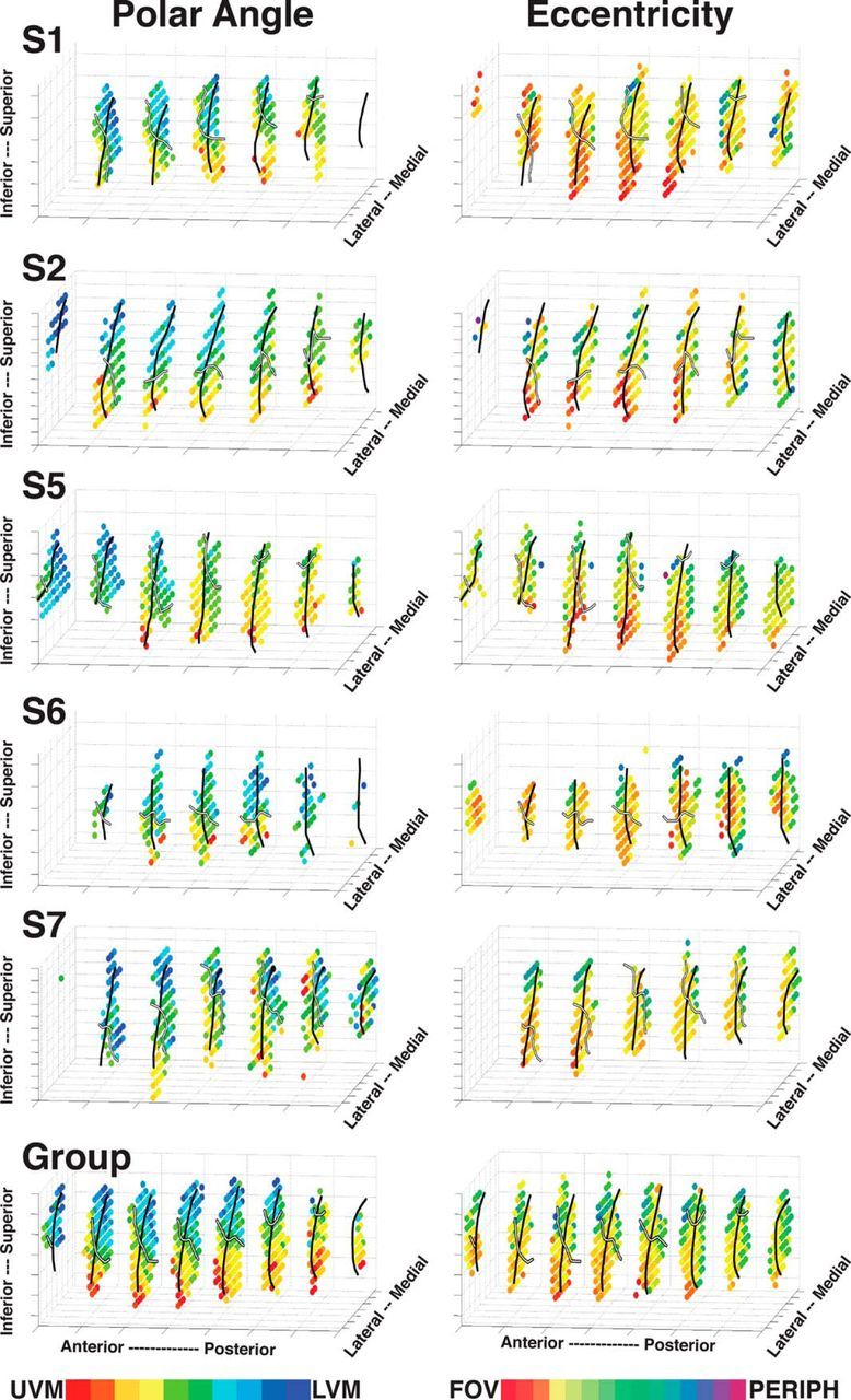
Three-dimensional (3D) plots of visual field representations within the ventral pulvinar. Polar angle (left) and eccentricity (right) phase maps are plotted for Subjects S1, S2, and S5–S7 and a group average (data collapsed across hemispheres). The data are not in a standardized space, and the spatial coordinates are arbitrary. Color code conventions are the same as in Figures 2 and 3, with the exception that ipsilateral representations are color coded black. Black solid line drawn on the individual subject and group average plots indicates the border between vPul1 and vPul2. White solid line indicates the HM.

Figure 11.

Thalamocortical functional connectivity for vPul1, vPul2, LGN, and medial pulvinar. Functional connectivity between 23 cortical areas and vPul1, vPul2, and LGN as well as anatomically defined medial pulvinar. Cortical regions are color coded based on anatomical regions: occipital cortex (blue), dorsal extrastriate (light green), parietal and frontal cortices (dark green), lateral temporal-occipital cortices (yellow), and ventral temporal cortex (red). *p < 0.05 (FDR-corrected, one-sample t tests).

Diffusion imaging.

All DWI and non-DWI were corrected for eddy currents and head motion using affine registration (12 df, FMRIB's Linear Registration Tool, FLIRT) to a non-DWI reference volume, geometrically unwarped with the field map scans, and then averaged to improve the signal-to-noise ratio (Jenkinson, 2001). The in-session structural scan was skull-stripped and registered (12 df) to the averaged and skull-stripped non-DWI reference scan to derive the transformation matrix between the two spaces.

Using FMRIB's DTIFIT tool, we calculated diffusion tensors for each voxel using linear least-squares fitting and diagonalized to obtain the voxel eigenvalues (λ₁, λ₂, λ₃) and eigenvectors. We created fractional anisotropy (FA) maps and color maps of principle orientation to visually check the major fiber orientations across the entire brain before proceeding to perform probabilistic diffusion tractography analyses (Mori and Barker, 1999).

Probabilistic diffusion tractography analyses were performed using FMRIB's Diffusion Toolkit, calculating probability distributions of fiber direction at each voxel (Behrens et al., 2003a; two fiber populations modeled per voxel, Behrens et al., 2003b). Tractography was performed in native diffusion space between visual cortex and the posterior thalamus in each hemisphere separately. An initial tractography analysis was performed to identify the most probable thalamic radiations connecting occipital, temporal, and frontal cortices with the pulvinar in each subject. Symmetrical tracking was performed where both the pulvinar and cortical ROIs were treated as masks. For each cortical region, a connectivity distribution (fdt_paths) was created that reflected the most probable fiber tract(s) between cortex and the pulvinar. Because of differences in the volumes of each area across subjects, the resulting tract estimates (fdt_paths) were normalized by the waytotal value (Rilling et al., 2008). The waytotal was calculated as the product of the number of voxels in the seed area and the number of individual tracts (samples) per voxel (5000). Normalized tracts were visually inspected, and a threshold of 0.01% of the total streamlines was chosen, which appeared to remove unlikely paths but maintain those that were anatomically plausible. In each subject, the entry points of the thalamic radiation were identified as the densest fiber tracts located adjacent to the pulvinar. To evaluate the consistency of these fiber tracts across subjects, each subject's thresholded paths were binarized, transformed into a standard (MNI) space, and converted to percentage overlap across subjects.

A second tracking analysis was performed between individual cortical visuotopic areas and the pulvinar. Probabilistic tracts were required to pass through any of the thalamic radiation entry points localized in each subject's initial tracking analysis and were restricted from crossing hemispheres. For this analysis, the pulvinar and surrounding white matter were treated as the seed mask, and each cortical area was treated as a target region. Cortical retinotopic mapping and delayed saccade tasks were used to identify 23 visuotopic areas spanning occipital, temporal, parietal, and frontal cortices: V1, V2, V3, hV4, VO1, VO2, PHC1, PHC2, LO1, LO2, TO1, TO2, V3A, V3B, IPS0, IPS1, IPS2, IPS3, IPS4, IPS5, SPL1, PreCC/SFS, and PreCC/IFS (for review of areas, see Silver and Kastner, 2009; Wandell and Winawer, 2011). For each cortical area tracking, each voxel in the pulvinar mask had a connectivity value representing the number of samples that passed through that given voxel. Because connectivity values can be affected by factors, such as size of target (cortical) areas, crossing fibers, and inhomogeneous signal-to-noise ratio across the brain, data were normalized by calculating a ratio of the connectivity value for each pulvinar voxel with a given cortical area (e.g., between hV4 and the pulvinar) to the highest connectivity value across all voxels in the pulvinar for that particular tracking. Ratios were calculated for each of the 23 cortical areas probed separately. Individual subject anatomical volumes were then aligned using the two-step registration procedure outlined above, and each subject's thalamocortical anatomical connectivity maps were transformed into MNI space. Data were then averaged across subjects to derive group average thalamic connectivity maps for each cortical area. To ensure that the group average connectivity patterns were evident in individual subjects, data in individual subjects were also visualized at a threshold ratio of 0.50 (i.e., any given thalamus voxel had to have a connectivity value at least 50% that of the maximum voxel estimate for that particular tracking).

Resting state.

Functional data were slice-time and motion corrected. In preparation for functional connectivity analyses, several additional steps were performed on the data: (1) removal of potential “spike” artifacts using AFNI's 3dDespike; (2) temporal filtering retaining frequencies in the 0.01–0.1 Hz band; (3) linear and quadratic detrending; and (4) removal by regression of several sources of variance: (1) the six motion parameter estimates and their temporal derivatives, (2) the signal from a ventricular region, and (3) the signal from a white matter region. Global mean signal removal was not included in the reported analyses given concerns about negative correlations (Fox et al., 2009; Murphy et al., 2009), although global mean signal removal yielded similar connectivity results. To minimize the effects due to the scanner onset, the initial 12 TRs (21.6 s) were removed from each eyes closed and fixation scan. For cortical areas, all voxels that fell within the gray matter were mapped to surface nodes.

We applied correlation analyses to identify cortical areas whose profile of correlations with all other cortical areas (referred to as cortical connectivity profile) was similar to the cortical connectivity profiles of individual voxels in the posterior thalamus. Analyses were performed on the same 23 cortical visuotopic areas used in the anatomical connectivity analyses. To identify the cortical connectivity profile of individual cortical areas, the mean time-series of each cortical area was correlated with the mean time-series of every other cortical area in each subject. To identify the cortical connectivity profile of the posterior thalamus in each subject, the mean time-series of each cortical area was correlated with the time-series of each voxel within a mask of the posterior thalamus that included the LGN, pulvinar, and surrounding white matter.

Next, we compared the cortical connectivity profiles of individual thalamus voxels with those of individual cortical areas. For each subject, the cortical connectivity profile of each thalamus voxel was correlated to a group average cortical connectivity profile of each cortical area, where the group average excluded that subject. This yielded a measurement of similarity between each cortical area's cortical connectivity profile and every thalamus voxel's cortical connectivity profile, which we refer to as the thalamocortical functional connectivity profile. Significant positive similarity in the thalamocortical functional connectivity profile was taken as evidence for connectivity between a thalamus voxel and a given cortical area. In a few cases, there was significant dissimilarity in the connectivity profile between a thalamus voxel and a given area. Our predictions were specifically tied to finding significant similarity. In cases of dissimilarity, we do not offer an interpretation, although we assume that these regions are not strongly coupled. Individual subject anatomical volumes were then aligned using the two-step registration procedure outlined above, and each subject's thalamocortical functional connectivity profile was transformed into MNI space. Voxelwise, one sample t tests were used to assess statistical significance.

To assess the cortical connectivity profiles of individual thalamic visual field maps (LGN, vPul1, and vPul2), the thalamocortical functional connectivity profiles of all voxels within each area (defined by the group average topographic mapping data) were averaged. The connectivity profile of a portion of the medial pulvinar that did not show significant topographic representations was also assessed.

Results

Anatomical parcellation of the thalamus

High-resolution anatomical images were used to distinguish several thalamic structures (Figs. 1, 2). The initial anatomical characterization of each individual's thalamus helped guide the interpretation of subsequent analyses directed at functional and diffusion tensor imaging data. In each subject, we identified the pulvinar as well as the LGN and medial geniculate nucleus (MGN) by inspection. These structures had lower T1 intensity values, thus appearing darker than the surrounding tissue. At 1.0 mm resolution, the boundaries between these thalamic structures were blurry. At 0.5 mm resolution, we were able to better resolve the boundaries between these structures (see Subjects S1 and S2 vs Subjects S3 and S4 in Figs. 1, 2). To verify the relative locations of thalamic structures, data were compared with very high-resolution (200 μm) histology images of an individual (Amunts et al., 2013) and with a group average MNI-152 template brain (Grabner et al., 2006) (Fig. 1). An anatomical parcellation of the thalamus based on the Morel stereotactic atlas (Morel et al., 1997; Krauth et al., 2010) was also used as a reference.

Figure 2.

Visuotopic representations within the anatomical extent of subcortical structures. The anatomical extent of the pulvinar, LGN, MGN, and SC is outlined in green, yellow, magenta, and blue, respectively, for Subjects S1–S4 in axial and two sagittal orientations. Below the anatomical segmentations, polar angle maps are presented in corresponding slices. The color code represents the phase of the fMRI response and indicates the region of the contralateral visual field to which the voxel responds best. The color code is mirror symmetrical between hemispheres, and ipsilateral representations are not color coded.

Anatomical pulvinar

The pulvinar (green arrows) was identified as a region of low T1 intensity (dark gray voxels) relative to surrounding tissue in the posterior-most part of the thalamus (Fig. 1). As seen in axial and sagittal slices (Fig. 1), the lateral anterior border of the ventral pulvinar abutted the posterior extent of the LGN with a thin strip of relatively higher T1 intensities falling in between the two nuclei. The two nuclei were most easily distinguishable in sagittal slices. Individual layers of the LGN were visible in the histology and provided a clear distinction from the pulvinar that lacked such layer structure (Fig. 1). The anterior border of the dorsal pulvinar was less clear and exhibited a gradual transition to higher T1 intensities (light gray voxels). As seen in coronal slices (Fig. 1), a gradual transition to higher T1 intensities was also observed lateral to the pulvinar within adjacent white matter. The midpoints of the gradual transition were interpreted as the lateral border of the pulvinar. As seen in sagittal and coronal slices (Fig. 1), the medial and posterior border of the pulvinar was identified at a sharp transition to very low T1 intensities (black voxels), marking a transition into the ambient cistern and third ventricle. As seen in coronal and sagittal slices (Fig. 1), the posterior ventral border of the pulvinar was identified at a transition to a thin strip of higher T1 intensities (light gray voxels), marking part of the brachium of the SC, before a sharp change to very low T1 intensities (black voxels) within a cavity of CSF. The borders of the pulvinar were sharper in the 0.5 mm resolution anatomical images but were also identifiable in the 1.0 mm images, and the extent of the pulvinar from both resolutions was near-identical in individual subjects. The borders were consistent with the anatomical extent of the pulvinar in histological images of an individual (Amunts et al., 2013), the group average MNI brain (Grabner et al., 2006), as well as the group average anatomical parcellation of the pulvinar using the Morel stereotactic atlas (Morel et al., 1997; Krauth et al., 2010).

Anatomy of additional subcortical structures

The LGN (Fig. 1, yellow arrow) was identified as a small area of low T1 intensity (dark gray voxels) relative to the surrounding tissue in the ventral thalamus. As seen in axial and sagittal slices (Fig. 1), the lateral and anterior borders of the LGN were defined at transitions to higher T1 intensity (light gray voxels) and marked the boundaries between the optic radiation and the posterior limb of the internal capsule, respectively. The posterior border of the LGN largely abutted the ventral pulvinar, although a thin strip of relatively higher T1 intensity (light gray voxels) was apparent in between the two nuclei in several sagittal slices for most subjects. As seen in sagittal slices, the ventral border of the LGN was identified at a sharp transition to very low T1 signal (black voxels) within a cavity of CSF separating the thalamus from parahippocampal cortex. In several subjects, a blood vessel (bright white voxels) was identified just below the LGN (Fig. 1, coronal images). The MGN (Fig. 1, magenta arrows) was identified as a small area of low T1 intensity (dark gray voxels) medial to the LGN. As seen in the axial slices, a strip of relatively higher T1 intensities (light gray voxels) separated the MGN from the LGN. The posterior border was defined at a transition to higher T1 intensities (light gray voxels) that marked the brachium of the SC. The borders of the MGN and LGN were consistent with histological images of an individual (Amunts et al., 2013), the group average MNI brain, as well as the group average anatomical parcellation of the pulvinar using the Morel stereotactic atlas (Morel et al., 1997; Krauth et al., 2010).

Polar angle and eccentricity mapping in the thalamus

Bilateral activations within the posterior thalamus were found in all subjects for the polar angle and eccentricity mapping studies. Activations within each hemisphere were mainly confined to the contralateral hemifield. Activation maps of polar angle and eccentricity for individual subjects are shown overlaid on T1-weighted anatomical images of the thalamus (Figs. 2, 3). The color of each voxel was determined by the phase of its response and indicates the region of the contralateral visual field to which the voxel was most responsive. For the polar angle component, the upper visual field (UVF) is denoted in red-yellow, the horizontal meridian (HM) in green, and the lower visual field (LVF) in blue. For each hemisphere, only contralateral activations are color coded. For the eccentricity measurements, the central space is denoted in red-orange (<4°), the midfield in yellow-green (4°–9°), and periphery in blue-purple (9°–15°).

Figure 3.

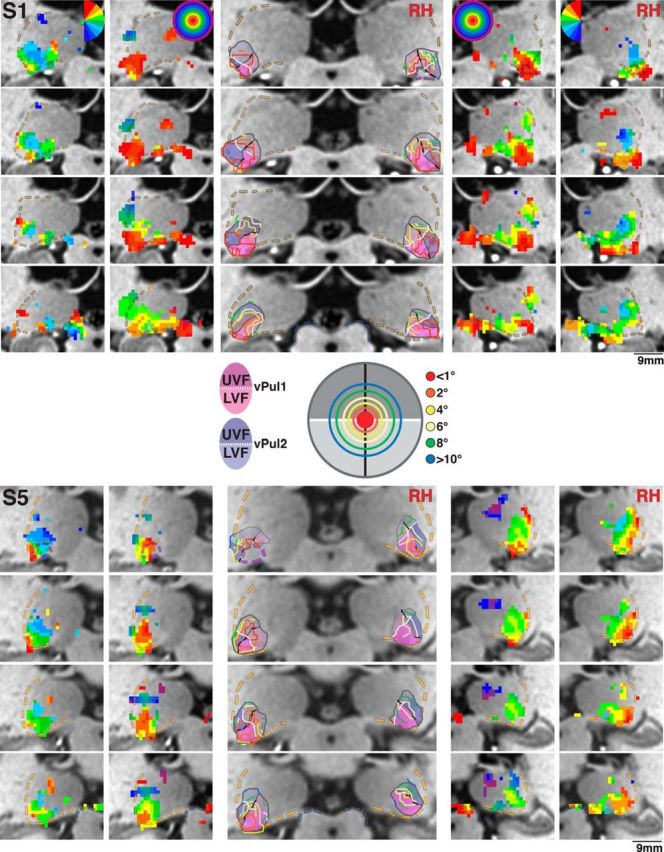
Polar angle and eccentricity maps of the human pulvinar for Subjects S1 and S5. Series of coronal views of polar angle (outer columns) and eccentricity (intermediate columns) phase maps presented anterior (top) to posterior (bottom) in 1 mm spacing for right and left hemispheres. Transparent yellow and blue dashed lines indicate the lateral border of the pulvinar and the superior border of the SC, respectively. Transparent purple dashed lines in the anterior-most slice of S1 (right hemisphere) and S5 (left hemisphere) indicate the posterior anatomical extent of the LGN. Color code conventions are the same as Figure 2. Centrally presented images illustrate the color code of iso-eccentricity contours along 1°, 2°, 4°, 6°, 8°, and 10°. Transparent shading in centrally presented anatomical slices represents the extent of vPul1 (blue) and vPul2 (red) and their UVF (dark shading) and LVF (light shading) representations. White line indicates the HM.

We identified four visual field maps of contralateral space within human subcortex in all 9 subjects. Two visual field maps were located within the ventral pulvinar. In addition, we identified visual field maps in the LGN and SC, consistent with prior studies from our laboratory and others (Schneider et al., 2004; Schneider and Kastner, 2005; Katyal et al., 2010). Activations outside of the anatomical extent of these subcortical structures were not evaluated (but see DeSimone et al., 2015). We also observed contralateral representations within the medial ventral and dorsal lateral pulvinar, although these visual field representations varied across subjects.

Ventral pulvinar

We identified representations of the contralateral visual space within the lateral half of the ventral pulvinar in each subject (Figs. 2–6). A representation of the UVF (red-yellow voxels) was identified within inferior-most and lateral portions of the ventral pulvinar (Figs. 2, 3). Representations of the UVF were contiguous from lateral-most to ventromedial portions of the pulvinar, although two peaks in the UVF representation, one ventral and the other lateral, were observed in several hemispheres (10 of 18). As seen in sagittal and coronal slices (Figs. 2, 3), a phase progression was observed from this UVF representation to a representation of the LVF located dorsomedially (blue voxels). A thin strip of HM representation (green voxels) was consistently identified in between the UVF and LVF representation in each subject. As seen in the coronal slices (Fig. 3, middle columns, white line), the HM was typically oriented ventromedial to dorsolateral, and as seen in sagittal slices (e.g., Fig. 2, Subject S4) from ventroanterior to dorsoposterior, with the UVF representation located slightly posterior to the LVF representation (Fig. 2).

Figure 5.

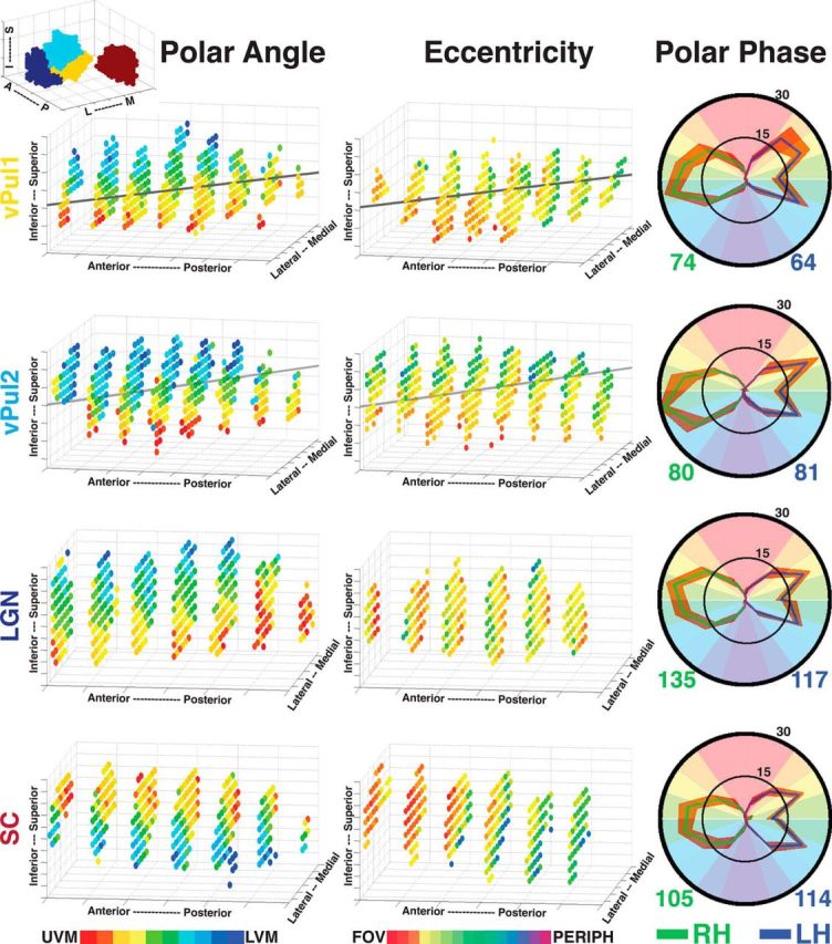
Visual field representations in areas vPul1, vPul2, LGN, and SC. Group average 3D polar angle (left) and eccentricity (middle) maps are plotted for vPul1, vPul2, LGN, and SC. Transparent gray line indicates the AIR for vPul1 and vPul2. Top left 3D plot illustrates the relative locations of the LGN (dark blue), vPul1 (yellow), vPul2 (light blue), and SC (red). Polar phase plots (right) illustrate the distribution of polar angle representations for each subcortical area (thresholded at p < 0.05, uncorrected). The percentage of polar angle coverage (see Materials and Methods) within each area was calculated for subjects individually and then averaged. Solid green and blue lines indicate group averages from right and left hemispheres, respectively. Orange outline indicates the SEM variance. Numbers below each polar plot reflect the average volume in mm³ for each hemisphere.

Figure 6.

Group average polar angle and eccentricity maps in the human pulvinar. Series of coronal views of group average polar angle (N = 9) and eccentricity (N = 5) phase maps presented in MNI coordinates. Borders of anatomically defined lateral, inferior, and medial pulvinar subdivisions are denoted by transparent black dashed lines in each image and are highlighted in centrally presented anatomical images (Morel et al., 1997; Krauth et al., 2010). An average subject anatomical image is used as the underlay for the phase maps. Centrally presented images illustrate color coded iso-eccentricity contours (for details, see Fig. 3). All other conventions are the same as in Figures 2 and 3.

Eccentricity representations were observed in the ventral pulvinar and generally overlapped with polar angle maps (Fig. 3, intermediate columns). As seen in coronal slices, a large representation of central space (red/orange voxels) was identified within the ventral pulvinar. In all subjects, this representation of central space spanned several millimeters anterior to posterior and was typically located in the middle of the polar angle maps. Representations of mid-eccentricities (yellow/green) surrounded the central representations in each hemisphere of the 5 subjects probed and extended to peripheral representations (blue/purple) in at least one hemisphere for 4 subjects. A distinct representation of peripheral space was also identified in the dorsal, lateral pulvinar in at least one hemisphere for 4 subjects (e.g., RH of Subject S5) and was considered separate from the eccentricity representations within the ventral pulvinar.

The location of central and peripheral representations relative to the polar angle maps suggests that portions of the ventral pulvinar dorsolateral and ventromedial to the foveal representation contain redundant representations of the visual field and likely are part of separate visual field maps. To test this, the polar angle phase progression was evaluated along contours of iso-eccentricity (Fig. 3, middle column). Contours of iso-eccentricity were identified at least partially in each subject (see Materials and Methods). First, iso-eccentricity contours were identified for central-most representations in each coronal slice (Fig. 3, middle column, red/orange contours) followed by mid-eccentricity (yellow/green) and then peripheral representations (blue). In some coronal slices, there was no clear, distinct peak in the representation of central space (<1°; e.g., top two slices in RH of Subject S5). In these cases, iso-contour lines were drawn around representations of central space that fell most clearly within the ventral pulvinar and that were contiguous with the representations of central space in neighboring (e.g., posterior) coronal slices. In each subject, reversals in polar angle progression at or near the vertical meridians (red/yellow or blue polar angle voxels) were identified for several iso-eccentricity contours (Fig. 3, middle column, dark black lines). Reversal points spanned ventrolateral and dorsomedial portions of the phase maps in all subjects and generally separated the ventral pulvinar into ventromedial and dorsolateral halves, which we refer to as vPul1 and vPul2, respectively. Polar angle phase reversal line segments were connected to form the border between vPul1 and vPul2 (Fig. 3, middle columns, gray lines). Points in between the line segments were interpolated based on: (1) the general orientation of the border across coronal slices, (2) intersecting iso-eccentricity contours at approximately orthogonal orientations, and (3) generally minimizing the distance between line segments. The extent of vPul1 and vPul2 was constrained by the peripheral-most representations that surrounded the shared representation of central space (Fig. 3, middle columns, gray outlines). Specifically, the medial extent of vPul1 was typically identified at or near peripheral-most representations, and often corresponded to a reversal in eccentricity phase progression as seen in the RH of Subject S1 (Fig. 3). Likewise, the dorsolateral extent of vPul2 was typically identified at peripheral-most representations of visual space and corresponded to a reversal in eccentricity phase progression in a few hemispheres as seen in the RH of Subject S5 (Fig. 3). Any visual field representations beyond these peripheral-most representations were not included within the borders of vPul1 and vPul2. In several subjects, the ventrolateral extent of the (anatomical) pulvinar contained representations of central space. In these cases, the ventrolateral border of vPul2 was constrained by the boundary of the pulvinar gray. In a few hemispheres, the eccentricity phase progression was coarse, and these medial and lateral borders were identified at or near discontinuities in the eccentricity phase maps as seen in the LH of Subject S1. Based on the anatomical consistency of the foveal representation in these 5 subjects and relation to the polar angle reversal points, we approximated the location of the foveal representation and border between vPul1/2 in the remaining 4 subjects. The organization of iso-eccentricity, polar angle reversal points, and extent of vPul1 and vPul2 appeared symmetrical between hemispheres and were generally consistent across subjects.

The progression of contralateral visual space from UVF to LVF traverses anterior–posterior, superior–inferior, and lateral–medial planes (Figs. 2, 3). In most subjects, any given slice orientation only conveyed part of the polar angle and eccentricity phase progressions (Figs. 2, 3). To better visualize the organization of vPul1 and vPul2 (combined), phase values were plotted in 3 dimensions for individual subjects without the underlying anatomy (Fig. 4). To highlight the consistency of the visuotopic organization across hemispheres and between subjects, individual subject polar angle and eccentricity phase data within vPul1 and vPul2 were collapsed across hemispheres, and group averages were derived (see Materials and Methods). For individual subjects, the upper visual field was located ventrolaterally and the lower visual field was located dorsomedially. In most cases, the distribution of lower visual field representations was slightly more anterior than that of the upper visual field. In all cases, the middle area of polar angle maps was comprised of representations of central space (red/yellow) and was surrounded by midfield and peripheral representations (green/blue) along both the ventromedial and dorsolateral extents. In most cases, the central-most representations (red/orange) were also situated at or near the ventrolateral pole, particularly at anterior portions, and generally corresponded to representations of the upper visual field. Representations of central space (orange) were also observed in dorsomedial portions of the ventral pulvinar, which corresponded to representations of the lower visual field. Together, our data suggest that the representation of visual space extends from the UVF located caudal-infero-lateral to the LVF located rostro-supero-medial. The group average polar angle and eccentricity organization of the ventral pulvinar was similar to individual subjects, supporting the distinction of dorsolateral and ventromedial regions into separate visual field maps: vPul1 and vPul2 (Fig. 4, bottom row; see Materials and Methods). Group average 3D plots were then re-created for vPul1 and vPul2 separately by aligning the centroids of each individual map across subjects (Fig. 5). While the polar angle organization was similar between vPul1 and vPul2, the eccentricity organization showed clear differences with peripheral-most representations of vPul1 located more medially, and peripheral-most representations of vPul2 located more laterally. Overall, the general organization of polar angle and eccentricity 3D plots was consistent with the organization observed in individual subject coronal slices, providing additional support that the ventral pulvinar contains two visual field maps, vPul1 and vPul2, which are symmetrical between hemispheres.

An axis of iso-representation (AIR) runs perpendicular to the gradient of visual field representations in vPul1 and vPul2. A representation of the visual field, such as V1, is inherently two-dimensional, stretching along the cortical surface with iso-representations across layers within the same cortical column (Shipp, 2003). For the pulvinar, which lacks layers, a pseudo-coronal plane oriented caudo-infero-lateral to rostro-supero-medial contains a near-complete representation of the visual field, and the AIR is oriented perpendicular to this plane, running rostro-infero-lateral to caudo-supero-medial. This was verified by identifying AIR vectors for several portions of the visual field in vPul1 and vPul2 separately (see Materials and Methods). The average of these vectors is plotted for vPul1 and vPul2 in Figure 5 (transparent gray lines). The most prominent plane of the AIR was posterior–anterior, consistent with observing near-complete representations of visual space in pseudo-coronal slices. Part of the lateral–medial angle of the AIR could be attributed to the anatomy of the pulvinar gray shifting medially in posterior slices. The superior–inferior axis of the AIR could be explained in part by a superior shift of the pulvinar gray at posterior slices. However, the superior–inferior axis of the AIR is also influenced by head rotation (more than the other two planes). Variance in rotation was minimized across subjects by aligning the anterior and posterior commissures. Together, the AIR for both vPul1 and vPul2 appears to be linear and similar to the rostrolateral to caudomedial axis reported in the Old World monkeys (Shipp, 2001, 2003).

The mean volumes of vPul1 and vPul2 (n = 18) activated by the rotating wedge stimulus were 69 ± 14 mm³ and 80 ± 14 mm³, respectively, and were significantly correlated between hemispheres (across subjects): r = 0.78; p = 0.012 and r = 0.76; p = 0.017, respectively. As seen in the polar phase plots (Fig. 5, right column), the percentage of voxels representing 90° centered on the horizontal meridian was larger than the percentage representing the combined upper and lower 45° of contralateral visual space for both vPul1 (mean percentage 64% vs 34 ± 7% SD) and vPul2 (69% vs 31 ± 9% SD). The difference between vertical and horizontal meridian representations is likely due to a selective undersampling of the vertical meridian as a result of partial volume effects where voxels that sample from the vertical meridian likely also sample from contralateral representations off the vertical meridian (Haacke et al., 1994; Logothetis et al., 2002), and has been observed in previous imaging studies of the thalamus (Schneider et al., 2004; Schneider and Kastner, 2005). This compression toward the HM and under-representation of the VM may explain why the UVM and LVM were typically discontiguous. The percentage of voxels representing the upper and lower quadrants did not significantly differ (paired t test, ts < 1.72, p > 0.05). The group mean MNI coordinates for the centers of vPul1 maps in right and left hemispheres were −21, 29, −3 and 21, 29, −3, respectively. The group mean MNI coordinates for the centers of vPul2 maps in right and left hemispheres were −24, 30, 1 and 23, 31, 1, respectively. At their maximal extents, each visual field map spanned an average of 5 mm in the anterior–posterior, 5 mm lateral–medial, and 6 mm inferior–superior axes.

Dorsolateral and ventromedial pulvinar

In addition to the two visual field maps within the lateral half of the ventral pulvinar, representations of contralateral visual space were consistently observed in other parts of the pulvinar. These representations tended to be more variable across subjects. In 12 of 18 hemispheres, representations of contralateral visual space were identified dorsal to vPul2 (see Subjects S2–S4 in Fig. 2; RH Subjects S1 and S2, LH S5 in Fig. 3). In most cases, the UVF was located lateral to the LVF (see RH Subjects S1 and S5 in Fig. 3). In 6 of 10 hemispheres, a representation of central space, distinct from the central space representation shared by vPul1 and vPul2, was identified within this region of the dorsal pulvinar (see RH Subjects S1 and S5 in Fig. 3). In 10 of 18 hemispheres, representations of the contralateral visual field were identified in the ventral pulvinar medial to vPul1 (see Subjects S1 and S5 in Fig. 3). The relation of UVF to LVF in this region of the pulvinar was variable across subjects. The borders between these regions and vPul1 and vPul2 contained representations of the midfield and periphery. Although any organization of these contralateral representations was difficult to discern, these data suggest that both dorsal lateral and ventral medial pulvinar contain additional, coarse topographic representations of contralateral visual space. Future imaging studies at even higher spatial resolutions may better resolve the topography in these regions.

LGN

A representation of the contralateral visual field was identified within the anatomically defined LGN in all subjects. A representation of the LVF (blue voxels) was identified along the anterior, dorsal medial border of the LGN (Fig. 2). A phase progression was observed from this LVF representation to a representation of the UVF (red-yellow voxels) along the posterior, ventral lateral border. The LGN contained a large representation of central space along its medial side and progressed laterally to representations of the midfield and periphery. The organization of polar angle and eccentricity maps in the LGN is illustrated in the group average 3D plots (Fig. 5). The mean volume of each LGN (n = 18) activated by the rotating wedge stimulus was 126 ± 21 mm³ and was significantly correlated between hemispheres (r = 0.86; p < 0.01). As seen in the polar plots (Fig. 5), the percentage of voxels representing 90° centered on the horizontal meridian was larger than the percentage representing the combined upper and lower 45° of contralateral visual space (mean percentage 66% vs 34 ± 10% SD). The percentage of voxels representing the upper and lower quadrants did not significantly differ (paired t test, t < 1.8, p > 0.05). The group mean MNI coordinates for the centers of the LGN maps in right and left hemispheres were −24, 25, −6 and 24, 25, −6, respectively. The LGN spanned an average of 6 mm in the anterior–posterior, lateral–medial, and inferior–superior axes. The topographic organization of the LGN is in agreement with prior measurements at a coarser spatial resolution (Schneider et al., 2004). The volumetric measurements of the LGN are consistent with prior anatomical studies of the LGN (Andrews et al., 1997; Li et al., 2012).

Superior colliculus

A representation of the contralateral visual field was identified within the SC in all subjects (Fig. 2). A representation of the UVF (red-yellow) was identified along the anterior, dorsal medial border. A phase progression was observed from this UVF representation to a representation of the LVF (blue) along the posterior, ventral lateral border. A representation of central space was identified at the anterior, dorsolateral extent with increasingly peripheral representations located at the posterior, ventromedial extent. As would be expected, phase progressions did not extend into the inferior colliculus. The organization of polar angle and eccentricity maps in the SC is illustrated in the group average 3D plots (Fig. 5). The mean volume of each SC (n = 18) activated by the rotating wedge stimulus was 109 ± 23 mm³ and was significantly correlated between hemispheres (r = 0.82; p < 0.01). As seen in the polar plots (Fig. 5), the percentage of voxels representing 90° centered on the horizontal meridian was larger than the percentage representing the combined upper and lower 45° of contralateral visual space (mean percentage 65% vs 35 ± 11% SD). The percentage of voxels representing the upper and lower quadrants did not significantly differ (paired t test, t < 1.1, p > 0.05). The group mean MNI coordinates for the centers of the SC maps in right and left hemispheres were −5, 33, −3 and 5, 33, −3, respectively. The SC spanned an average of 4 mm in the anterior–posterior, 7 mm lateral–medial, and 6 mm inferior–superior axes. The topographic organization of the SC is in agreement with prior measurements at coarser spatial resolutions (Schneider and Kastner, 2005; Katyal et al., 2010).

Group average map

To further evaluate the consistency of the visuotopic organization across individuals, polar angle and eccentricity data were anatomically coregistered across subjects in MNI space (see Materials and Methods), and group average phase maps were calculated for each hemisphere. The organization of group average topographic maps for vPul1 and vPul2 (as well as the LGN and SC) was very similar to the organization observed in individual subjects (Fig. 6). Representations of contralateral visual space in dorsolateral and ventromedial regions of the pulvinar were evident in the group data as well. We compared these group average phase maps with lateral, inferior, and medial anatomical parcellations of the pulvinar based on the Morel stereotactic atlas (Morel et al., 1997; Krauth et al., 2010). The group average data covered the inferior pulvinar and most of the lateral pulvinar, as defined by the Morel atlas, but also extended into lateral and inferior portions of the medial pulvinar. vPul1 overlapped with the inferior pulvinar, a small part of the lateral pulvinar, and also extended into the medial pulvinar at the LVF representation. vPul2 mostly covered the ventral half of the lateral pulvinar but also extended into the medial pulvinar at the LVF representation. The representation of central space shared by vPul1 and vPul2 was located near the border of the lateral and inferior pulvinar in both hemispheres and extended a few millimeters into ventral portions of the medial pulvinar in the right hemisphere. As with the individual subject analysis, polar angle phase reversals were identified along iso-eccentricity contours (Fig. 6, middle columns). Representations of contralateral visual space were also apparent in the dorsal half of the lateral pulvinar and the medial half of the ventral pulvinar. As with the individual subject data, the topographic organization within these regions was difficult to discern. Overall, the group average phase maps also support the distinction of two visual field maps within the lateral half of the ventral pulvinar and provide additional evidence for some topographic organization of contralateral visual space within the dorsolateral and ventromedial portions of the ventral pulvinar.

The organization of thalamocortical connectivity

Anatomical thalamocortical connectivity

To investigate the organization of anatomical connectivity between the pulvinar and visual cortex, probabilistic analyses on diffusion tensor imaging data were conducted between the thalamus and 23 visuotopic cortical areas: V1, V2, V3, hV4, VO1, VO2, PHC1, PHC2, LO1, LO2, TO1, TO2, V3A, V3B, IPS0, IPS1, IPS2, IPS3, IPS4, IPS5, SPL1, PreCC/SFS, and PreCC/IFS (see Materials and Methods). Only ipsilateral (within hemisphere) connectivity patterns were assessed. An initial probabilistic tracking analysis of occipital, ventral temporal, lateral temporal-occipital, and parietal cortices revealed the fiber tracts leading into the posterior thalamus in each subject (Fig. 7A). This tracking did not include the optic radiation connecting the LGN with visual cortex. Each of these regional fiber tracts was similar across subjects. The parietal fiber tracts entered the thalamus via the superior thalamic radiation. The occipital and temporal tracts entered the thalamus via the posterior thalamic radiation. These fiber tracts were largely consistent with a previous tractography study of the human pulvinar (Leh et al., 2008). A second tracking analysis was conducted between each cortical area and the pulvinar (including surrounding white matter) with tracts constrained to the thalamic radiation identified in the initial analysis that interconnect the pulvinar and cortex. Ipsilateral connectivity patterns for individual areas were symmetrical between hemispheres (Figs. 7B, 8). Notably, the fiber tracts from cortex more reliably tracked through the white matter. For all connectivity maps, the largest connectivity values were located along the periphery of the posterior thalamus and within the surrounding white matter with lower connectivity values extending into the gray of the pulvinar nucleus. This pattern was also apparent in individual subjects and is likely due to fiber tracts becoming more disperse upon entering the pulvinar gray, effectively diluting the diffusion signal. Within the pulvinar nucleus, the connectivity maps for early visual and extrastriate areas V1–3, hV4, V3A-B, LO1–2, VO1–2, and PHC1–2 were similar. As seen for V1, V2, and hV4, the largest connectivity values were observed in the ventral pulvinar (Fig. 7B). These anatomical connectivity maps partially overlapped the group average vPul1 and vPul2 maps (data not shown; but see Fig. 10). Connectivity maps for ventral temporal areas VO1–2 and PHC1–2 also overlapped with the posterior medial pulvinar (Fig. 8, right column). As seen for TO1, the largest connectivity values for motion-sensitive areas (hMT⁺) (Amano et al., 2009) within lateral temporal-occipital cortex (TO1–2) were also within the ventral pulvinar and partially overlapped vPul1 and vPul2 (Figs. 7B, 8, left column). The connectivity maps for IPS1–5, SPL1, PreCC/SFS, and PreCC/IFS were similar to each other. As seen for IPS3, the largest connectivity values were within the dorsal pulvinar (Fig. 7B). Interestingly, the connectivity map for parietal area IPS0 (data not shown) was more similar to visual and extrastriate occipital areas than to the other parietal areas, with the highest probabilities located within the ventral pulvinar.

Figure 7.

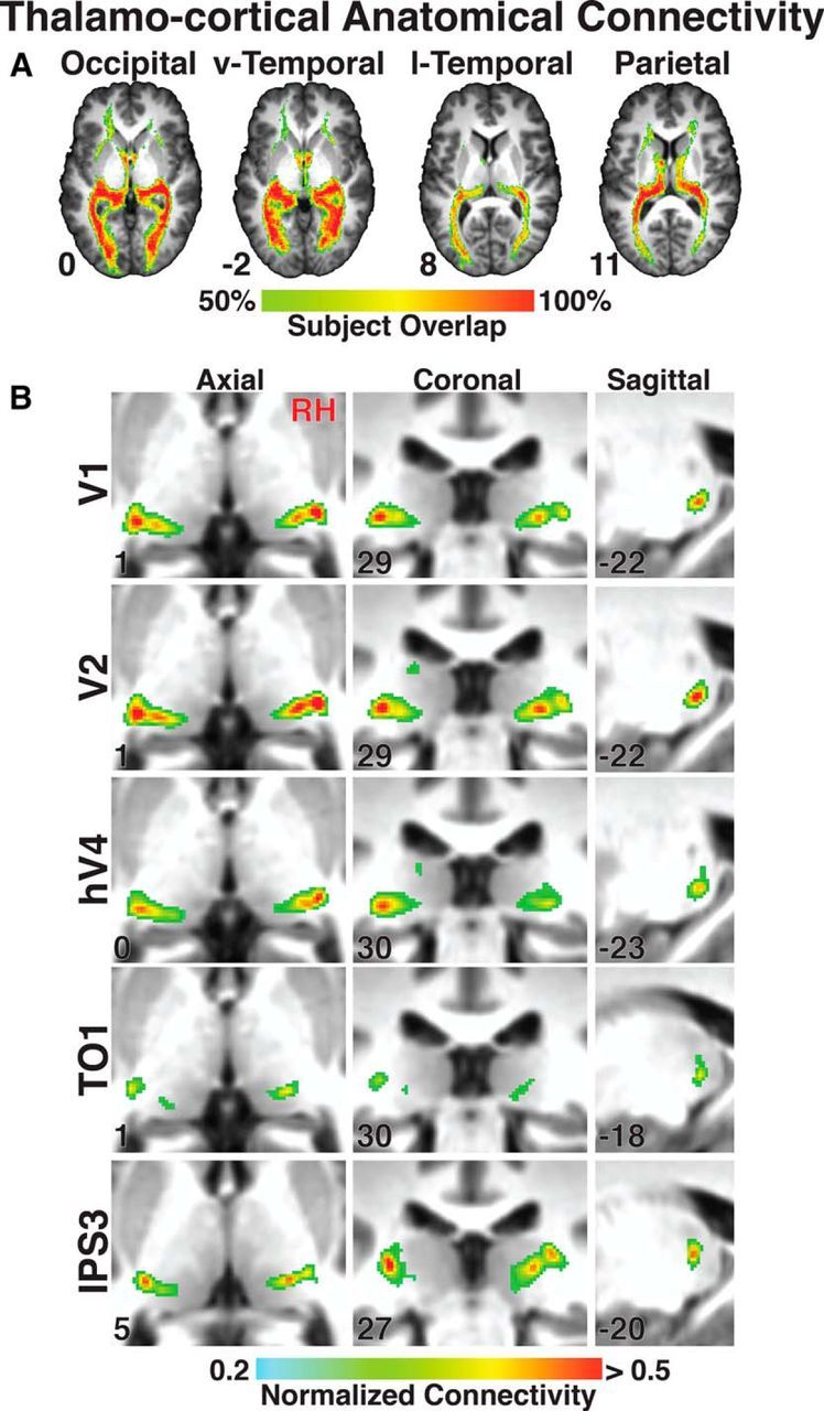
Thalamocortical anatomical connectivity of the human pulvinar. A, Subject overlap percentage maps of thalamocortical tracts between the pulvinar and occipital, ventral temporal, lateral temporal-occipital, and parietal cortex. Slices are presented in MNI space with corresponding axial slice coordinates. B, Group average (N = 14) peak anatomical connectivity of V1, V2, hV4, TO1, and IPS3 within the pulvinar in axial, coronal, and sagittal orientations. A standard MNI brain is used as the underlay, and coordinates are inset in each image.

Figure 8.

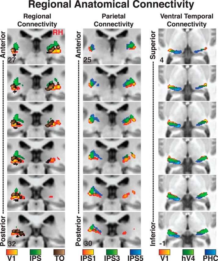
Regional thalamocortical anatomical connectivity of the human pulvinar. Relation of peak connectivity for V1, IPS, and TO in the pulvinar (left column). Relation of peak connectivity for IPS1, IPS3, and IPS5 in the dorsal pulvinar (center). Relation of the peak connectivity for V1, hV4, and PHC in the ventral pulvinar (right column). Coronal images are presented at 1 mm spacing. A standard MNI brain is used as the underlay, and coordinates are inset in the top and bottom images.

Figure 10.

Relation of anatomical and functional connectivity within the human pulvinar. Anatomical (dark blue) and functional (red) connectivity and their overlap (green) are shown in a series of coronal views for V1, TO, and IPS. *Mark peaks in connectivity. Outlines of topographic regions vPul1 (yellow), vPul2 (light blue), ventral medial pulvinar (orange), and dorsal lateral pulvinar (purple) are overlaid. Solid black lines indicate the boundary between vPul1 and vPul2. A standard MNI brain is used as the underlay, and coordinates are inset in the top and bottom images.

There were also clear regional differences in the connectivity maps (Fig. 8). The connectivity maps for posterior occipital cortex (V1, red/yellow voxels) and parietal cortex (combined IPS1–5, green voxels) were within the ventral and dorsal pulvinar, respectively (Fig. 8, left column). The connectivity maps were anatomically distinct from one another with minimal overlap. The connectivity maps for lateral temporal-occipital cortex (combined TO1–2, brown voxels) fell in between posterior occipital and parietal maps and extended into the ventral medial pulvinar. Within the dorsal pulvinar, there was a ventrolateral to dorsomedial gradient of connectivity from posterior parietal cortex (IPS1, red/yellow voxels) to anterior parietal cortex (IPS5, blue voxels) (Fig. 8, middle column). Intermediate parietal cortex (such as IPS3, green voxels) fell in between and heavily overlapped both anterior and posterior parietal connectivity maps. Within the ventral pulvinar, there was a rostrolateral to caudomedial gradient of connectivity from occipital cortex (V1, red/yellow voxels) to ventral temporal cortex (combined PHC1–2, blue voxels) (Fig. 8, right column). Connectivity maps for intermediate ventral temporal areas, such as hV4 (green voxels), fell in between and heavily overlapped with both posterior occipital and anterior ventral temporal connectivity maps. We assessed the gradient of connectivity from early visual to ventral temporal cortex by identifying the best-fitting line from a regression on the spatial coordinates of the peak connectivity for V1, hV4, and PHC. This analysis was similar to the AIR analysis on the retinotopy data (see Materials and Methods). The resulting vector was oriented rostrolateral to caudomedial. This gradient of anatomical projections is consistent with the rostro-infero-lateral to caudo-supero-medial AIR (axis of iso-representation) observed in the 3D visual field map plots (Figs. 4, 5). Together, these data demonstrate a topographic organization of cortical anatomical connections in the pulvinar and a clear distinction in the cortical connectivity patterns between dorsal and ventral portions of the pulvinar.

Functional thalamocortical connectivity

To investigate the organization of functional connectivity (temporal covariance in BOLD signal) between the pulvinar and visual cortex, correlations were performed on task-free, resting state data between the thalamus and the same 23 cortical areas explored in the anatomical connectivity analyses (see Materials and Methods). Only ipsilateral connectivity patterns were assessed. The mean time-series in each cortical area was correlated with the time-series of every voxel within a mask of the posterior thalamus that included the LGN, pulvinar, and adjacent white matter (Fig. 9A). For most cortical areas, the mean time-series was positively correlated with the time-series of many voxels in the posterior thalamus. In addition, most cortical areas were positively correlated with each other, making it difficult to evaluate the specificity of the correlated signal. For example, V1 and V2 were both positively correlated with the LGN (as well as with the pulvinar). However, V1 and V2 were also positively correlated with each other. Assuming that BOLD functional connectivity reflects both direct and indirect anatomical connectivity (Vincent et al., 2007; Honey et al., 2009), it is difficult to assess the correlated signal between the LGN and V2. We assumed that signals between directly connected areas should be more correlated than between indirect or weakly connected areas. Indeed, the correlation between V1 and the LGN was stronger than the correlation between V2 and the LGN. Therefore, we reasoned that using the full pattern of functional correlations across all areas (cortical connectivity profile) should be a more sensitive measure (vs pairwise correlations). Cortical connectivity profiles should be more similar for areas that are directly (vs indirectly) connected. To explore this, we first calculated a cortical connectivity profile for each cortical area (e.g., V1's average correlation with all other cortical areas) as well as a cortical connectivity profile for all thalamus voxels that reflected the strength of correlation with each of the 23 cortical areas (Fig. 9A; see Materials and Methods). In each subject, the cortical connectivity profile of each thalamus voxel was then correlated with the (leaving that subject out) group average cortical connectivity profile for each cortical area, yielding a measurement of how similar each thalamus voxel's cortical connectivity profile was to each cortical area's cortical connectivity profile. This measurement is referred to as the thalamocortical connectivity profile. The spatial pattern of each area's thalamocortical connectivity profile within the thalamus was qualitatively similar and highly correlated between eyes closed and fixation conditions (all r values > 0.70). Data were then averaged across conditions to increase signal-to-noise in individual subject data. To evaluate the consistency of these thalamocortical profiles across individuals, subjects were anatomically coregistered, and connectivity profiles were averaged to yield group data. For each cortical visual area, there was a cluster of thalamus voxels with positive thalamocortical connectivity profile correlations that significantly differed from zero across subjects (p < 0.01, two-tailed).

Figure 9.

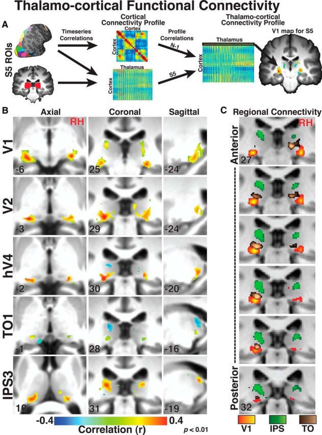
Thalamocortical functional connectivity in the human pulvinar. A, Diagram of functional connectivity analysis pipeline for an individual subject (for more details, see Materials and Methods). B, Group average (N = 13) peak functional connectivity within the pulvinar for V1, V2, hV4, TO1, and IPS3. C, Relation of peak connectivity for V1, IPS, and TO in the pulvinar. A standard MNI brain is used as the underlay, and coordinates are inset individual images.

The spatial patterns of these ipsilateral thalamocortical connectivity profiles (functional connectivity maps) were symmetrical between hemispheres but varied across cortical areas (Fig. 9B). Across subjects, the cortical connectivity profile of V1 was most strongly correlated with the cortical connectivity profile of voxels within the LGN but was also positively correlated with the connectivity profile of voxels within the ventral pulvinar as well as a region in the dorsal thalamus, anterior and adjacent to the medial pulvinar, which may correspond to the lateral posterior nucleus based on comparisons to the Morel stereotactic atlas (Morel et al., 1997; Krauth et al., 2010). In contrast, the cortical connectivity profiles of extrastriate areas V2, V3, hV4, V3A-B, LO1–2, VO1–2, and PHC1–2 were most strongly correlated with the connectivity profile of voxels in the ventral pulvinar, just posterior to the LGN. As shown for areas V2 (but also hV4), this was particularly evident in sagittal slice orientations where strong correlations were observed in the anatomical extent of the ventral pulvinar, but not the LGN (Fig. 9B). The functional connectivity maps for these extrastriate areas overlapped within the ventral pulvinar (Fig. 9B) and were located almost entirely within the group average vPul1 and vPul2 maps (data not shown; but see Figs. 10, 11). The funcitonal connectivity map of PHC2 (data not shown; but see Fig. 11) also overlapped with posterior portions of the medial pulvinar and the dorsal lateral pulvinar. As shown for TO1, the functional connectivity maps of lateral temporal-occipital cortex areas (TO1–2) partially overlapped with V1-hV4 connectivity, but also overlapped with medial portions of the ventral pulvinar, anterior to the functional connectivity maps of ventral temporal areas (Fig. 9B). Although significant, the peak magnitudes of the TO1–2 connectivity maps were weaker than other area maps. This could reflect relatively weaker or more diffuse connectivity but could also reflect variance in regional signal quality within the pulvinar and across cortex as well as signal differences due to differences in areal size. For these reasons, we interpret the location of the peaks in the functional connectivity maps as being more informative than the relative magnitude of the peaks. As shown for IPS3, the cortical connectivity profiles of parietal and frontal areas, IPS1–5, SPL1, PreCC/SFS, and PreCC/IFS, were most strongly correlated with the connectivity profile of voxels within the dorsal pulvinar (Fig. 9B). Interestingly, this region of the dorsal pulvinar did not overlap with vPul1, vPul2, or the additional topographic representations within the dorsal lateral pulvinar and ventral medial pulvinar (data not shown; but see Figs. 10, 11). As with the anatomical data, the functional connectivity map for IPS0 (data not shown) was more similar to visual and extrastriate areas than the other parietal areas, with correlations strongest in the ventral pulvinar. Also similar to the anatomical connectivity, there were regional differences in thalamocortical functional connectivity between posterior occipital (V1, red/yellow voxels), parietal (combined IPS1–5, green voxels), and lateral temporal-occipital cortex (combined TO1–2, brown voxels) cortex (Fig. 9C). Together, there was a clear distinction in the thalamocortical functional connectivity patterns between dorsal and ventral portions of the pulvinar.

Comparison of anatomical and functional connectivity patterns

Despite measuring very different signals in the brain, anatomical and functional connectivity methods demonstrated strikingly similar broad spatial patterns within the pulvinar, largely distinguishing the ventral and dorsal pulvinar (Figs. 8, 9C). However, the anatomical and functional thalamocortical connectivity maps of any individual area only partially overlapped, and the peaks of each map (asterisks) were typically offset by a few millimeters (Fig. 10). Interestingly, there appeared to be a systematic relationship between these maps and their peak offsets. As seen in Figure 10, the anatomical connectivity maps (blue voxels) for posterior occipital (V1, left column), lateral temporal-occipital (combined TO1–2, middle column), and parietal (combined IPS1–5, right column) cortices extended from adjacent white matter into the pulvinar gray and abutted or partially overlapped (green voxels) the peak functional connectivity (red voxels). The overlap between functional and anatomical connectivity almost always excluded the peaks of connectivity (asterisks). Further, the functional connectivity maps of occipital areas, such as V1-hV4, fell almost entirely within the extent of the group average vPul1 (yellow outline) and vPul2 (light blue outline) maps, whereas the anatomical connectivity partially overlapped with the visual field maps but also overlapped with the surrounding white matter. The anatomical connectivity maps of lateral temporal-occipital areas mainly overlapped with the dorsal-most portion of the topographic maps as well as adjacent white matter. The functional connectivity maps of lateral temporal-occipital areas partially overlapped with vPul1–2 but also overlapped with ventral medial portions of the pulvinar that showed coarse representations of contralateral space (orange outline). The peaks of these functional connectivity maps were located within this ventral medial region of the pulvinar and its border with vPul1. Functional and anatomical maps of parietal cortex minimally overlapped with any topographic representations in the pulvinar. Although the subject pools for functional and anatomical data were not entirely overlapping, this pattern was also evident in individual subjects and in group data restricted to a completely overlapping subject pool (data not shown), suggesting that these differences reflect the intrinsic organization of these functional and anatomical signals.

Functional connectivity of subcortical fieldmaps

Given that our topographic data appeared in better correspondence with the functional connectivity data than the anatomical connectivity data, we assessed the strength of thalamocortical functional connectivity in the LGN, vPul1, and vPul2 (as defined by the group average mapping data), as well as a region of the medial pulvinar that did not show significant visuotopic representations (Fig. 11). Across subjects, the cortical connectivity pattern of the LGN was most similar to the cortical connectivity pattern of visual area V1 (p < 0.05, FDR corrected). In contrast, the cortical connectivity patterns of vPul1 and vPul2 were similar to the cortical connectivity patterns of several visual areas: V1-hV4, VO1–2, and PHC1–2 (p < 0.05, FDR corrected). The thalamocortical connectivity patterns for vPul1 and vPul2 were very similar, although the similarity with early visual areas (V1–3) was slightly more pronounced (relative to other cortical areas) in vPul1. The cortical connectivity profile of the medial pulvinar was most similar to the cortical connectivity profiles of parietal areas IPS1–5, and SPL1, as well as frontal areas PreCC/SFS, and PreCC/IFS (p < 0.05, FDR corrected). The cortical connectivity profile of the medial pulvinar was also similar to PHC2 and visual area V1 (p < 0.05, FDR corrected). These data converge with observations from the voxelwise analyses and highlight a general differentiation in cortical connectivity patterns between the LGN and pulvinar as well as between portions of the pulvinar that showed consistent topographic organization and portions that did not.

Comparison to organization of macaque pulvinar

The visuotopic organization of the human pulvinar has strong similarities with the organization of the pulvinar in other primate species (Fig. 12). Two maps of visual space have been identified in the ventral pulvinar of several primate species: (1) an inferior map referred to as P1 or VP1 and (2) a lateral map referred to as P2 or VP2 (Gattass et al., 1978; Bender, 1981; Li et al., 2013). In our human data, the more medial map, vPul1, appears to correspond to the P1/VP1 map in macaques, and the more lateral map, vPul2, appears to correspond to P2/VP2. Additional representations of contralateral visual space were identified within the ventral medial and dorsal lateral pulvinar, which may correspond to regions P3 and P4 of the macaque, respectively (Gattass et al., 2014; Ungerleider et al., 2014). To compare our mapping results with the visuotopic organization of the macaque pulvinar, we color coded receptive fields from recording sites within the macaque ventral pulvinar (adapted from Bender, 1981) as a function of their polar angle and eccentricity representations using a color code with a similar gradient as our fMRI data (see Materials and Methods). The general topographic organization of both maps is similar between species (Fig. 12). The representation of the visual field is inverted in these two maps with upper visual space represented ventrally and lower visual space represented dorsally. The two maps border each other at the LVM and share a common representation of central space that spans several millimeters in the anterior–posterior direction. In both species, the lateral map is almost entirely within the anatomically defined lateral subdivision of the ventral pulvinar, whereas the more medial, inferior map overlaps with both the anatomically defined lateral and inferior subdivisions (Morel et al., 1997; Shipp, 2003). These similarities were most apparent in comparisons with the topographic organization of the anterior half of the macaque ventral pulvinar (Fig. 12, left column).

Figure 12.

Comparison of the topographic organization within the ventral pulvinar between humans and macaques. Comparison of fMRI-defined polar angle (top half) and eccentricity (bottom half) representations within the human ventral pulvinar (left side) with electrophysiologically defined topographic organization of the macaque pulvinar (right side). Adapted from Bender (1981). The macaque coronal images show visual field coverage from electrode penetrations spanning anterior (A) to posterior (D) slices of the pulvinar. See axial slice inset for relative anterior/posterior positions of each coronal slice. Coronal images A and B illustrate the retinotopic organization of the inferior pulvinar and the anterior half of the lateral pulvinar. Coronal images C and D illustrate the retinotopic organization of the posterior half of the lateral pulvinar. Color code conventions are the same as Figure 2 and are matched between species.

There were, however, possible differences between our human data and more posterior portions of the macaque pulvinar (Fig. 12, right column). In particular, the lateral map in the macaque ventral pulvinar (P2/VP2) contains a second-order representation of the visual field in which there is a split in the visual field representation at the HM, such as seen in cortical area V2 (Bender, 1981; Shipp, 2003). As a key feature of this organization, the lateral extent of the posterior pulvinar is comprised of a representation of the HM, and the lateral map folds over the inferior map with the split in the HM forming both the lateral and ventral borders of the pulvinar (Fig. 12) (Bender, 1981). Such organization was less apparent in our human data (Figs. 2–6, 12). Consistent with the macaque organization, the HM extends to the lateral border of vPul2. However, the ventral, lateral border of vPul2 mainly contains representations of the upper visual field. Further, representations of the UVF (red/yellow) are located lateral to the HM in vPul2 (boundary between light and dark green voxels; Figs. 2–6, 12). These differences are not likely due to inaccuracies in our data, as these features of the visuotopic organization of vPul1 and vPul2 were consistent in individual subjects as well as in the group average data. The VM (vs HM) was underrepresented in our human data, which is likely due to a partial volume-sampling artifact (Fig. 5; see Retinotopic mapping). If anything, this artifact should have biased vPul2 to have more of a HM representation along the lateral border. As such, it is possible to interpret the visual field of vPul2 as a first-order representation, such as V1 as well as for all human visual field maps anterior to area V3 (Wandell et al., 2005). Although speculative, such variation between species could reflect differences in the topographic organization and morphology of visual cortex, which has extensive, reciprocal connections with the pulvinar. Alternatively, the HM representation near the posterior lateral border of the pulvinar may split vPul2 into dorsal and ventral halves and form a second-order representation similar to P2 in macaques (Fig. 13A). Although the HM representation along the lateral border of the pulvinar appears to be less extensive in our data compared with macaques (Fig. 12), the relatively larger receptive fields within the posterior pulvinar (Bender, 1981) may have limited our ability to precisely image this aspect of the pulvinar's visuotopic organization. Further studies at higher spatial resolution and scanner field strength may resolve these possible species differences.

Figure 13.

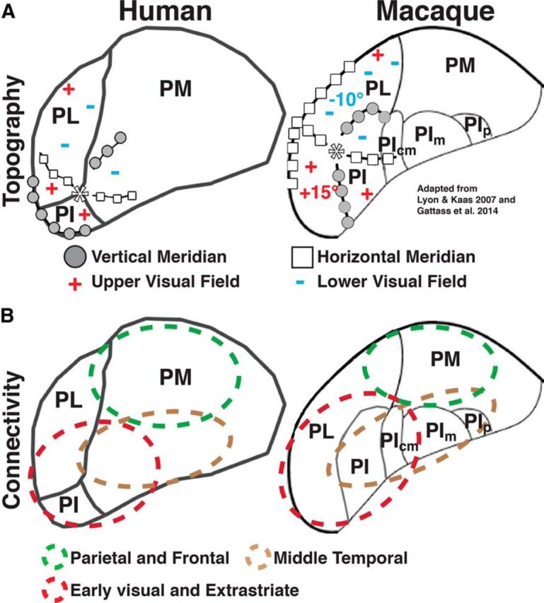
Schematic of the topographic organization and cortical connectivity of the pulvinar between humans and macaque. A, Schematic of the visual field organization in the pulvinar in humans and macaques. Adapted from Kaas and Lyon (2007) and Gattass et al. (2014). Inferior, lateral, and medial subdivisions in the human pulvinar were adapted from Morel et al. (1997). Because of the significant underrepresentation of the vertical meridian in our fMRI data, portions of the border between vPUL1/2 were inferred at points closest to the vertical meridian that corresponded to reversals in phase progression along iso-eccentricity contours. *Mark foveal representations. Shaded circles represent the vertical meridian. White boxes represent the horizontal meridian. +, Upper visual field; −, lower visual field. B, Schematic of regional cortical connectivity patterns in the pulvinar in humans and macaques. Red dashed lines indicate early visual and extrastriate connectivity. Brown dashed lines indicate middle temporal (lateral occipital/temporal in humans) connectivity. Green dashed lines indicate parietal and frontal connectivity. The anterior to posterior gradient of anatomical connections from early visual to ventral temporal cortex is not illustrated in this figure.

Connectivity patterns in the human pulvinar resembled the known anatomical connectivity in monkeys (Fig. 13B). The two ventral visual field maps are strongly connected with occipital and temporal cortex in humans and other primate species (Gutierrez et al., 1995; Adams et al., 2000; Shipp, 2003). The connectivity of the anterior-most temporal area we investigated (PHC2) overlapped with these two maps but also extended into the posterior-most parts of the medial pulvinar, consistent with connectivity patterns of anterior ventral temporal cortex in other primate species (Benevento and Rezak, 1976; Baleydier and Morel, 1992; Baizer et al., 1993). Beyond these two maps, we identified coarse representations of contralateral space within the dorsal lateral and ventral medial pulvinar in humans. The representations within the ventral medial pulvinar overlapped peaks of connectivity with motion-sensitive areas TO1–2 (Amano et al., 2009). In other primate species, this region of the medial ventral pulvinar also contains some contralateral tuning (Bender, 1981; Li et al., 2013) and is interconnected with motion-sensitive regions (Standage and Benevento, 1983; Ungerleider et al., 1984; Shipp, 2003; Berman and Wurtz, 2010). The dorsal medial pulvinar did not show clear contralateral tuning and was mainly interconnected with parietal and frontal cortex in humans. This is comparable with the organization of the dorsal medial pulvinar in other primates (Yeterian and Pandya, 1985; Schmahmann and Pandya, 1990; Benevento and Port, 1995; Gutierrez et al., 2000; Wilke et al., 2010).

Discussion

We investigated the anatomical and functional organization of the human pulvinar in a series of experiments using a variety of approaches, including high-resolution anatomical imaging, retinotopic mapping, functional connectivity analyses on task-free resting-state data, and anatomical connectivity analyses on diffusion imaging data. By considering both the polar angle and eccentricity phase maps, we identified two visual field maps within the ventral pulvinar, which we labeled vPul1 and vPul2. The organization of these two maps was highly consistent across subjects. We also found evidence for coarse visuotopic organization within the dorsal lateral and ventral medial pulvinar. Functional and anatomical connectivity was investigated between the thalamus and 23 cortical visuotopic areas across occipital, temporal, parietal, and frontal cortices. Connectivity patterns yielded striking differences between dorsal and ventral regions of the pulvinar, as well as between the pulvinar and the LGN. Together, these data provide new insight into the functional and anatomical organization of the human pulvinar.

Our results demonstrate the existence of several representations of contralateral visual space in the human pulvinar, thereby confirming previous reports that had suggested topographic organization within the human pulvinar (Cotton and Smith, 2007; Schneider, 2011; DeSimone et al., 2015). Using a very high-resolution scanning sequence, we were able to identify two visual field maps, vPul1 and vPul2, within the lateral half of the ventral pulvinar. The location of vPul1 and vPul2 appeared to correspond well with previous reports of visually evoked activity in the human ventral pulvinar (Cotton and Smith, 2007; Schneider, 2011). The organization of these two maps is similar to other primate species, although some differences were observed (Bender, 1981; Shipp, 2003). The two maps share a common foveal representation and a contiguous eccentricity representation. Cortical regions with such an organization have been proposed to form a functional cluster with the computations of individual maps related to common perceptual processes (Wandell et al., 2005). Thus, we propose that the visual field map cluster hypothesis extends to thalamic organization, and the functions within these two areas share a similar computational goal. The ventral medial and dorsal lateral pulvinar contained additional representations of contralateral visual space with eccentricity representations distinct from vPul1/2. Thus, these regions of the pulvinar likely are not part of the vPul1/2 cluster and may support different perceptual processes. A previous study from our laboratory only found activation within the dorsal pulvinar during a spatial attention task when subjects attended to targets in both visual hemifields (Kastner et al., 2004). The coarser voxel resolution used in that study likely limited the ability to identify these two visuotopic maps in the ventral pulvinar. However, the location of activation in the dorsal pulvinar from this prior work matches our parietal and frontal functional connectivity results and falls outside regions that showed strong contralateral tuning in our mapping experiment. Given this connectivity, it is likely that this region of the dorsal pulvinar contains large receptive fields that span much of the visual field, including ipsilateral space, and may contain some coarse visuotopic organization. Revealing any such organization likely will require the combination of even higher sampling resolution and higher (7T+) MR field strengths.

Our results clarify and extend previous studies on thalamocortical connectivity in humans. Several studies have segmented the human thalamus and other subcortical structures based on anatomical connectivity using broad cortical targets (e.g., entire sensory and association cortical regions) (Behrens et al., 2003b; Johansen-Berg et al., 2005; Zhang et al., 2010). Our investigations of connectivity used 23 cortical areas, functionally defined in individual subjects, as specific targets to allow a more fine-grained view of the pulvinar's connectivity. Functional and anatomical connectivity analyses yielded converging results. Striate and extrastriate visual cortex was most strongly connected with the ventral pulvinar with a rostrolateral to caudomedial gradient of connectivity from posterior occipital areas to ventral temporal areas (Shipp, 2003). A region of the ventral pulvinar medial to vPul1 was also connected with motion-sensitive areas, TO1–2 (Amano et al., 2009), confirming a previous histochemical study of the human pulvinar that distinguished this region from lateral portions of the ventral pulvinar and identified it as possible zone for connectivity with motion-sensitive cortex (Cola et al., 1999). Parietal and frontal cortex was most strongly connected with the dorsal pulvinar with a lateral to medial gradient of connectivity from posterior to anterior parietal areas (Shipp, 2003). Furthermore, the observed spatial correspondence between peak foci in our functional and anatomical connectivity can explain previously reported dissociations between these two methods (Zhang et al., 2010). Overall, our functional connectivity data were in better spatial correspondence with the functionally defined topographic maps in the pulvinar gray, whereas the anatomical connectivity results showed regional specificity but appeared to be oriented toward fiber tract entry points from the surrounding white matter. This makes sense given the nature of the underlying signals analyzed for both approaches and suggests that these approaches are complementary, but dissociable in segmenting thalamic structures.

At a broader scale, our functional and anatomical connectivity results support the general distinction between dorsal and ventral portions of the pulvinar in primates (Baleydier and Morel, 1992; Baizer et al., 1993; Gutierrez et al., 2000; Shipp, 2003; Kaas and Lyon, 2007). Early visual and extrastriate cortical areas were most strongly connected with the ventral pulvinar. Parietal and frontal cortical areas were most strongly connected with the dorsal pulvinar. Aside from this distinction, the connectivity patterns of neighboring cortical areas were very similar with the foci of connectivity from neighboring areas heavily overlapping. Such overlap in connectivity has been observed in other primate species and is thought to provide a second, indirect pathway between cortically connected areas (Sherman and Guillery, 2002; Shipp, 2003). These connectivity results suggest that the human pulvinar, like other primates, is well positioned to regulate corticocortical communication (Jones, 2001; Shipp, 2003; Saalmann et al., 2012). Together, our results provide additional support that the general organization of the pulvinar is consistent across the primate phylogenetic tree.

References

- Adams MM, Hof PR, Gattass R, Webster MJ, Ungerleider LG. Visual cortical projections and chemoarchitecture of macaque monkey pulvinar. J Comp Neurol. 2000;419:377–393. doi: 10.1002/(SICI)1096-9861(20000410)419:3<377::AID-CNE9>3.0.CO%3B2-E. [DOI] [PubMed] [Google Scholar]
- Amano K, Wandell BA, Dumoulin SO. Visual field maps, population receptive field sizes, and visual field coverage in the human MT+ complex. J Neurophysiol. 2009;102:2704–2718. doi: 10.1152/jn.00102.2009. [DOI] [PMC free article] [PubMed] [Google Scholar]
- Amunts K, Lepage C, Borgeat L, Mohlberg H, Dickscheid T, Rousseau MÉ, Bludau S, Bazin PL, Lewis LB, Oros-Peusquens AM, Shah NJ, Lippert T, Zilles K, Evans AC. BigBrain: an ultrahigh-resolution 3D human brain model. Science. 2013;340:1472–1475. doi: 10.1126/science.1235381. [DOI] [PubMed] [Google Scholar]
- Andrews TJ, Halpern SD, Purves D. Correlated size variations in human visual cortex, lateral geniculate nucleus, and optic tract. J Neurosci. 1997;17:2859–2868. doi: 10.1523/JNEUROSCI.17-08-02859.1997. [DOI] [PMC free article] [PubMed] [Google Scholar]
- Arcaro MJ, McMains SA, Singer BD, Kastner S. Retinotopic organization of human ventral visual cortex. J Neurosci. 2009;29:10638–10652. doi: 10.1523/JNEUROSCI.2807-09.2009. [DOI] [PMC free article] [PubMed] [Google Scholar]
- Arcaro MJ, Pinsk MA, Li X, Kastner S. Visuotopic organization of macaque posterior parietal cortex: a functional magnetic resonance imaging study. J Neurosci. 2011;31:2064–2078. doi: 10.1523/JNEUROSCI.3334-10.2011. [DOI] [PMC free article] [PubMed] [Google Scholar]
- Baizer JS, Desimone R, Ungerleider LG. Comparison of subcortical connections of inferior temporal and posterior parietal cortex in monkeys. Vis Neurosci. 1993;10:59–72. doi: 10.1017/S0952523800003229. [DOI] [PubMed] [Google Scholar]
- Baleydier C, Morel A. Segregated thalamocortical pathways to inferior parietal and inferotemporal cortex in macaque monkey. Vis Neurosci. 1992;8:391–405. doi: 10.1017/S0952523800004922. [DOI] [PubMed] [Google Scholar]
- Bandettini PA, Jesmanowicz A, Wong EC, Hyde JS. Processing strategies for time-course data sets in functional MRI of the human brain. Magn Reson Med. 1993;30:161–173. doi: 10.1002/mrm.1910300204. [DOI] [PubMed] [Google Scholar]
- Behrens TE, Woolrich MW, Jenkinson M, Johansen-Berg H, Nunes RG, Clare S, Matthews PM, Brady JM, Smith SM. Characterization and propagation of uncertainty in diffusion-weighted MR imaging. Magn Reson Med. 2003a;50:1077–1088. doi: 10.1002/mrm.10609. [DOI] [PubMed] [Google Scholar]
- Behrens TE, Johansen-Berg H, Woolrich MW, Smith SM, Wheeler-Kingshott CA, Boulby PA, Barker GJ, Sillery EL, Sheehan K, Ciccarelli O, Thompson AJ, Brady JM, Matthews PM. Non-invasive mapping of connections between human thalamus and cortex using diffusion imaging. Nat Neurosci. 2003b;6:750–757. doi: 10.1038/nn1075. [DOI] [PubMed] [Google Scholar]
- Bender DB. Retinotopic organization of macaque pulvinar. J Neurophysiol. 1981;46:672–693. doi: 10.1152/jn.1981.46.3.672. [DOI] [PubMed] [Google Scholar]
- Benevento LA, Port JD. Single neurons with both form/color differential responses and saccade-related responses in the nonretinotopic pulvinar of the behaving macaque monkey. Vis Neurosci. 1995;12:523–544. doi: 10.1017/S0952523800008439. [DOI] [PubMed] [Google Scholar]
- Benevento LA, Rezak M. The cortical projections of the inferior pulvinar and adjacent lateral pulvinar in the rhesus monkey (Macaca mulatta): an autoradiographic study. Brain Res. 1976;108:1–24. doi: 10.1016/0006-8993(76)90160-8. [DOI] [PubMed] [Google Scholar]
- Berman RA, Wurtz RH. Functional identification of a pulvinar path from superior colliculus to cortical area MT. J Neurosci. 2010;30:6342–6354. doi: 10.1523/JNEUROSCI.6176-09.2010. [DOI] [PMC free article] [PubMed] [Google Scholar]
- Brainard DH. The Psychophysics Toolbox. Spat Vis. 1997;10:433–436. doi: 10.1163/156856897X00357. [DOI] [PubMed] [Google Scholar]
- Bressler DW, Silver MA. Spatial attention improves reliability of fMRI retinotopic mapping signals in occipital and parietal cortex. Neuroimage. 2010;53:526–533. doi: 10.1016/j.neuroimage.2010.06.063. [DOI] [PMC free article] [PubMed] [Google Scholar]
- Cola MG, Gray DN, Seltzer B, Cusick CG. Human thalamus: neurochemical mapping of inferior pulvinar complex. Neuroreport. 1999;10:3733–3738. doi: 10.1097/00001756-199912160-00002. [DOI] [PubMed] [Google Scholar]
- Cotton PL, Smith AT. Contralateral visual hemifield representations in the human pulvinar nucleus. J Neurophysiol. 2007;98:1600–1609. doi: 10.1152/jn.00419.2007. [DOI] [PubMed] [Google Scholar]
- Cox RW. AFNI: software for analysis and visualization of functional magnetic resonance neuroimages. Comput Biomed Res. 1996;29:162–173. doi: 10.1006/cbmr.1996.0014. [DOI] [PubMed] [Google Scholar]
- Cox RW, Jesmanowicz A. Real-time 3D image registration for functional MRI. Magn Reson Med. 1999;42:1014–1018. doi: 10.1002/(SICI)1522-2594(199912)42:6<1014::AID-MRM4>3.0.CO%3B2-F. [DOI] [PubMed] [Google Scholar]
- Dale AM, Fischl B, Sereno MI. Cortical surface-based analysis: I. Segmentation and surface reconstruction. Neuroimage. 1999;9:179–194. doi: 10.1006/nimg.1998.0395. [DOI] [PubMed] [Google Scholar]
- DeSimone K, Viviano J, Schneider K. Population receptive field estimation reveals new retinotopic maps in human. J Neurosci. 2015;35 doi: 10.1523/JNEUROSCI.3840-14.2015. xxx–xxx. [DOI] [PMC free article] [PubMed] [Google Scholar]
- Engel SA, Glover GH, Wandell BA. Retinotopic organization in human visual cortex and the spatial precision of functional MRI. Cereb Cortex. 1997;7:181–192. doi: 10.1093/cercor/7.2.181. [DOI] [PubMed] [Google Scholar]
- Fischl B, Sereno MI, Dale AM. Cortical surface-based analysis: II. Inflation, flattening, and a surface-based coordinate system. Neuroimage. 1999;9:195–207. doi: 10.1006/nimg.1998.0396. [DOI] [PubMed] [Google Scholar]
- Fox MD, Zhang D, Snyder AZ, Raichle ME. The global signal and observed anticorrelated resting state brain networks. J Neurophysiol. 2009;101:3270–3283. doi: 10.1152/jn.90777.2008. [DOI] [PMC free article] [PubMed] [Google Scholar]
- Gattass R, Oswaldo-Cruz E, Sousa AP. Visuotopic organization of the cebus pulvinar: a double representation the contralateral hemifield. Brain Res. 1978;152:1–16. doi: 10.1016/0006-8993(78)90130-0. [DOI] [PubMed] [Google Scholar]
- Gattass R, Galkin TW, Desimone R, Ungerleider LG. Subcortical connections of area V4 in the macaque. J Comp Neurol. 2014;522:1941–1965. doi: 10.1002/cne.23513. [DOI] [PMC free article] [PubMed] [Google Scholar]
- Grabner G, Janke AL, Budge MM, Smith D, Pruessner J, Collins DL. Symmetric atlasing and model based segmentation: an application to the hippocampus in older adults. Medical image computing and computer-assisted intervention: MICCAI International Conference on Medical Image Computing and Computer-Assisted Intervention. 2006;9:58–66. doi: 10.1007/11866763_8. [DOI] [PubMed] [Google Scholar]
- Gutierrez C, Yaun A, Cusick CG. Neurochemical subdivisions of the inferior pulvinar in macaque monkeys. J Comp Neurol. 1995;363:545–562. doi: 10.1002/cne.903630404. [DOI] [PubMed] [Google Scholar]
- Gutierrez C, Cola MG, Seltzer B, Cusick C. Neurochemical and connectional organization of the dorsal pulvinar complex in monkeys. J Comp Neurol. 2000;419:61–86. doi: 10.1002/(SICI)1096-9861(20000327)419:1<61::AID-CNE4>3.0.CO%3B2-I. [DOI] [PubMed] [Google Scholar]
- Haacke EM, Hopkins A, Lai S, Buckley P, Friedman L, Meltzer H, Hedera P, Friedland R, Klein S, Thompson L. 2D and 3D high resolution gradient echo functional imaging of the brain: venous contributions to signal in motor cortex studies. NMR Biomed. 1994;7:54–62. doi: 10.1002/nbm.1940070109. [DOI] [PubMed] [Google Scholar]
- Hansen KA, Kay KN, Gallant JL. Topographic organization in and near human visual area V4. J Neurosci. 2007;27:11896–11911. doi: 10.1523/JNEUROSCI.2991-07.2007. [DOI] [PMC free article] [PubMed] [Google Scholar]
- Honey CJ, Sporns O, Cammoun L, Gigandet X, Thiran JP, Meuli R, Hagmann P. Predicting human resting-state functional connectivity from structural connectivity. Proc Natl Acad Sci U S A. 2009;106:2035–2040. doi: 10.1073/pnas.0811168106. [DOI] [PMC free article] [PubMed] [Google Scholar]
- Jenkinson M. International Conference on Human Brain Mapping. Brighton, England: 2001. Improved unwarping of EPI volumes using regularised B0 maps. [Google Scholar]
- Jenkinson M. Fast, automated, N-dimensional phase-unwrapping algorithm. Magn Reson Med. 2003;49:193–197. doi: 10.1002/mrm.10354. [DOI] [PubMed] [Google Scholar]
- Jenkinson M, Beckmann CF, Behrens TE, Woolrich MW, Smith SM. Fsl. Neuroimage. 2012;62:782–790. doi: 10.1016/j.neuroimage.2011.09.015. [DOI] [PubMed] [Google Scholar]
- Jezzard P, Balaban RS. Correction for geometric distortion in echo planar images from B0 field variations. Magn Reson Med. 1995;34:65–73. doi: 10.1002/mrm.1910340111. [DOI] [PubMed] [Google Scholar]
- Johansen-Berg H, Behrens TE, Sillery E, Ciccarelli O, Thompson AJ, Smith SM, Matthews PM. Functional-anatomical validation and individual variation of diffusion tractography-based segmentation of the human thalamus. Cereb Cortex. 2005;15:31–39. doi: 10.1093/cercor/bhh105. [DOI] [PubMed] [Google Scholar]
- Jones EG. The thalamic matrix and thalamocortical synchrony. Trends Neurosci. 2001;24:595–601. doi: 10.1016/S0166-2236(00)01922-6. [DOI] [PubMed] [Google Scholar]
- Kaas JH, Lyon DC. Pulvinar contributions to the dorsal and ventral streams of visual processing in primates. Brain Res Rev. 2007;55:285–296. doi: 10.1016/j.brainresrev.2007.02.008. [DOI] [PMC free article] [PubMed] [Google Scholar]
- Kastner S, O'Connor DH, Fukui MM, Fehd HM, Herwig U, Pinsk MA. Functional imaging of the human lateral geniculate nucleus and pulvinar. J Neurophysiol. 2004;91:438–448. doi: 10.1152/jn.00553.2003. [DOI] [PubMed] [Google Scholar]
- Kastner S, DeSimone K, Konen CS, Szczepanski SM, Weiner KS, Schneider KA. Topographic maps in human frontal cortex revealed in memory-guided saccade and spatial working-memory tasks. J Neurophysiol. 2007;97:3494–3507. doi: 10.1152/jn.00010.2007. [DOI] [PubMed] [Google Scholar]
- Katyal S, Zughni S, Greene C, Ress D. Topography of covert visual attention in human superior colliculus. J Neurophysiol. 2010;104:3074–3083. doi: 10.1152/jn.00283.2010. [DOI] [PubMed] [Google Scholar]
- Konen CS, Kastner S. Two hierarchically organized neural systems for object information in human visual cortex. Nat Neurosci. 2008a;11:224–231. doi: 10.1038/nn2036. [DOI] [PubMed] [Google Scholar]
- Konen CS, Kastner S. Representation of eye movements and stimulus motion in topographically organized areas of human posterior parietal cortex. J Neurosci. 2008b;28:8361–8375. doi: 10.1523/JNEUROSCI.1930-08.2008. [DOI] [PMC free article] [PubMed] [Google Scholar]
- Krauth A, Blanc R, Poveda A, Jeanmonod D, Morel A, Székely G. A mean three-dimensional atlas of the human thalamus: generation from multiple histological data. Neuroimage. 2010;49:2053–2062. doi: 10.1016/j.neuroimage.2009.10.042. [DOI] [PubMed] [Google Scholar]
- Leh SE, Chakravarty MM, Ptito A. The connectivity of the human pulvinar: a diffusion tensor imaging tractography study. Int J Biomed Imaging. 2008;2008:789539. doi: 10.1155/2008/789539. [DOI] [PMC free article] [PubMed] [Google Scholar]
- Li K, Patel J, Purushothaman G, Marion RT, Casagrande VA. Retinotopic maps in the pulvinar of bush baby (Otolemur garnettii) J Comp Neurol. 2013;521:3432–3450. doi: 10.1002/cne.23358. [DOI] [PMC free article] [PubMed] [Google Scholar]
- Li M, He HG, Shi W, Li J, Lv B, Wang CH, Miao QW, Wang ZC, Wang NL, Walter M, Sabel BA. Quantification of the human lateral geniculate nucleus in vivo using MR imaging based on morphometry: volume loss with age. AJNR Am J Neuroradiol. 2012;33:915–921. doi: 10.3174/ajnr.A2884. [DOI] [PMC free article] [PubMed] [Google Scholar]
- Logothetis N, Merkle H, Augath M, Trinath T, Ugurbil K. Ultra high-resolution fMRI in monkeys with implanted RF coils. Neuron. 2002;35:227–242. doi: 10.1016/S0896-6273(02)00775-4. [DOI] [PubMed] [Google Scholar]
- Morel A, Magnin M, Jeanmonod D. Multiarchitectonic and stereotactic atlas of the human thalamus. J Comp Neurol. 1997;387:588–630. doi: 10.1002/(SICI)1096-9861(19971103)387:4<588::AID-CNE8>3.0.CO%3B2-Z. [DOI] [PubMed] [Google Scholar]
- Mori S, Barker PB. Diffusion magnetic resonance imaging: its principle and applications. Anat Rec. 1999;257:102–109. doi: 10.1002/(SICI)1097-0185(19990615)257:3<102::AID-AR7>3.0.CO%3B2-6. [DOI] [PubMed] [Google Scholar]
- Murphy K, Birn RM, Handwerker DA, Jones TB, Bandettini PA. The impact of global signal regression on resting state correlations: are anti-correlated networks introduced? Neuroimage. 2009;44:893–905. doi: 10.1016/j.neuroimage.2008.09.036. [DOI] [PMC free article] [PubMed] [Google Scholar]
- Olszewski J. Basel, Switzerland: Karger; 1952. The thalamus of the Macaca mulatta, an atlas for use with the stereotaxic instrument. [Google Scholar]
- Pelli DG. The VideoToolbox software for visual psychophysics: transforming numbers into movies. Spat Vis. 1997;10:437–442. doi: 10.1163/156856897X00366. [DOI] [PubMed] [Google Scholar]
- Reese TG, Heid O, Weisskoff RM, Wedeen VJ. Reduction of eddy-current-induced distortion in diffusion MRI using a twice-refocused spin echo. Magn Reson Med. 2003;49:177–182. doi: 10.1002/mrm.10308. [DOI] [PubMed] [Google Scholar]
- Rilling JK, Glasser MF, Preuss TM, Ma X, Zhao T, Hu X, Behrens TE. The evolution of the arcuate fasciculus revealed with comparative DTI. Nat Neurosci. 2008;11:426–428. doi: 10.1038/nn2072. [DOI] [PubMed] [Google Scholar]
- Saad ZS, Reynolds RC. Suma. Neuroimage. 2012;62:768–773. doi: 10.1016/j.neuroimage.2011.09.016. [DOI] [PMC free article] [PubMed] [Google Scholar]
- Saalmann YB, Kastner S. Cognitive and perceptual functions of the visual thalamus. Neuron. 2011;71:209–223. doi: 10.1016/j.neuron.2011.06.027. [DOI] [PMC free article] [PubMed] [Google Scholar]
- Saalmann YB, Pinsk MA, Wang L, Li X, Kastner S. The pulvinar regulates information transmission between cortical areas based on attention demands. Science. 2012;337:753–756. doi: 10.1126/science.1223082. [DOI] [PMC free article] [PubMed] [Google Scholar]
- Schira MM, Tyler CW, Breakspear M, Spehar B. The foveal confluence in human visual cortex. J Neurosci. 2009;29:9050–9058. doi: 10.1523/JNEUROSCI.1760-09.2009. [DOI] [PMC free article] [PubMed] [Google Scholar]
- Schmahmann JD, Pandya DN. Anatomical investigation of projections from thalamus to posterior parietal cortex in the rhesus monkey: a WGA-HRP and fluorescent tracer study. J Comp Neurol. 1990;295:299–326. doi: 10.1002/cne.902950212. [DOI] [PubMed] [Google Scholar]
- Schneider KA. Subcortical mechanisms of feature-based attention. J Neurosci. 2011;31:8643–8653. doi: 10.1523/JNEUROSCI.6274-10.2011. [DOI] [PMC free article] [PubMed] [Google Scholar]
- Schneider KA, Kastner S. Visual responses of the human superior colliculus: a high-resolution functional magnetic resonance imaging study. J Neurophysiol. 2005;94:2491–2503. doi: 10.1152/jn.00288.2005. [DOI] [PubMed] [Google Scholar]
- Schneider KA, Richter MC, Kastner S. Retinotopic organization and functional subdivisions of the human lateral geniculate nucleus: a high-resolution functional magnetic resonance imaging study. J Neurosci. 2004;24:8975–8985. doi: 10.1523/JNEUROSCI.2413-04.2004. [DOI] [PMC free article] [PubMed] [Google Scholar]
- Sereno MI, Pitzalis S, Martinez A. Mapping of contralateral space in retinotopic coordinates by a parietal cortical area in humans. Science. 2001;294:1350–1354. doi: 10.1126/science.1063695. [DOI] [PubMed] [Google Scholar]
- Sherman SM, Guillery RW. The role of the thalamus in the flow of information to the cortex. Philos Trans R Soc Lond B Biol Sci. 2002;357:1695–1708. doi: 10.1098/rstb.2002.1161. [DOI] [PMC free article] [PubMed] [Google Scholar]
- Shipp S. Corticopulvinar connections of areas V5, V4, and V3 in the macaque monkey: a dual model of retinal and cortical topographies. J Comp Neurol. 2001;439:469–490. doi: 10.1002/cne.1363. [DOI] [PubMed] [Google Scholar]
- Shipp S. The functional logic of cortico-pulvinar connections. Philos Trans R Soc Lond B Biol Sci. 2003;358:1605–1624. doi: 10.1098/rstb.2002.1213. [DOI] [PMC free article] [PubMed] [Google Scholar]
- Silver MA, Kastner S. Topographic maps in human frontal and parietal cortex. Trends Cogn Sci. 2009;13:488–495. doi: 10.1016/j.tics.2009.08.005. [DOI] [PMC free article] [PubMed] [Google Scholar]
- Smith SMB. SUSAN: a new approach to low level image processing. Int J Comput Vis. 1997;23:45–78. doi: 10.1023/A:1007963824710. [DOI] [Google Scholar]
- Smith SM, Jenkinson M, Woolrich MW, Beckmann CF, Behrens TE, Johansen-Berg H, Bannister PR, De Luca M, Drobnjak I, Flitney DE, Niazy RK, Saunders J, Vickers J, Zhang Y, De Stefano N, Brady JM, Matthews PM. Advances in functional and structural MR image analysis and implementation as FSL. Neuroimage. 2004;23(Suppl 1):S208–S219. doi: 10.1016/j.neuroimage.2004.07.051. [DOI] [PubMed] [Google Scholar]
- Standage GP, Benevento LA. The organization of connections between the pulvinar and visual area MT in the macaque monkey. Brain Res. 1983;262:288–294. doi: 10.1016/0006-8993(83)91020-X. [DOI] [PubMed] [Google Scholar]
- Stepniewska I, Kaas JH. Architectonic subdivisions of the inferior pulvinar in New World and Old World monkeys. Vis Neurosci. 1997;14:1043–1060. doi: 10.1017/S0952523800011767. [DOI] [PubMed] [Google Scholar]
- Swisher JD, Halko MA, Merabet LB, McMains SA, Somers DC. Visual topography of human intraparietal sulcus. J Neurosci. 2007;27:5326–5337. doi: 10.1523/JNEUROSCI.0991-07.2007. [DOI] [PMC free article] [PubMed] [Google Scholar]
- Ungerleider LG, Desimone R, Galkin TW, Mishkin M. Subcortical projections of area MT in the macaque. J Comp Neurol. 1984;223:368–386. doi: 10.1002/cne.902230304. [DOI] [PubMed] [Google Scholar]
- Ungerleider LG, Galkin TW, Desimone R, Gattass R. Subcortical projections of area V2 in the macaque. J Cogn Neurosci. 2014;26:1220–1233. doi: 10.1162/jocn_a_00571. [DOI] [PMC free article] [PubMed] [Google Scholar]
- Vincent JL, Patel GH, Fox MD, Snyder AZ, Baker JT, Van Essen DC, Zempel JM, Snyder LH, Corbetta M, Raichle ME. Intrinsic functional architecture in the anaesthetized monkey brain. Nature. 2007;447:83–86. doi: 10.1038/nature05758. [DOI] [PubMed] [Google Scholar]
- Wandell BA, Winawer J. Imaging retinotopic maps in the human brain. Vision Res. 2011;51:718–737. doi: 10.1016/j.visres.2010.08.004. [DOI] [PMC free article] [PubMed] [Google Scholar]
- Wandell BA, Brewer AA, Dougherty RF. Visual field map clusters in human cortex. Philos Trans R Soc Lond B Biol Sci. 2005;360:693–707. doi: 10.1098/rstb.2005.1628. [DOI] [PMC free article] [PubMed] [Google Scholar]
- Wang L, Mruczek RE, Arcaro MJ, Kastner S. Probabilistic maps of visual topography in human cortex. Cereb Cortex. 2014 doi: 10.1093/cercor/bhu277. doi: 10.1093/cercor/bhu277. Advance online publication. Retrieved Dec. 1, 2014. [DOI] [PMC free article] [PubMed] [Google Scholar]
- Wilke M, Turchi J, Smith K, Mishkin M, Leopold DA. Pulvinar inactivation disrupts selection of movement plans. J Neurosci. 2010;30:8650–8659. doi: 10.1523/JNEUROSCI.0953-10.2010. [DOI] [PMC free article] [PubMed] [Google Scholar]
- Woolrich MW, Jbabdi S, Patenaude B, Chappell M, Makni S, Behrens T, Beckmann C, Jenkinson M, Smith SM. Bayesian analysis of neuroimaging data in FSL. Neuroimage. 2009;45:S173–S186. doi: 10.1016/j.neuroimage.2008.10.055. [DOI] [PubMed] [Google Scholar]
- Yeterian EH, Pandya DN. Corticothalamic connections of the posterior parietal cortex in the rhesus monkey. J Comp Neurol. 1985;237:408–426. doi: 10.1002/cne.902370309. [DOI] [PubMed] [Google Scholar]
- Zhang D, Snyder AZ, Shimony JS, Fox MD, Raichle ME. Noninvasive functional and structural connectivity mapping of the human thalamocortical system. Cereb Cortex. 2010;20:1187–1194. doi: 10.1093/cercor/bhp182. [DOI] [PMC free article] [PubMed] [Google Scholar]
- Zhang Y, Brady M, Smith S. Segmentation of brain MR images through a hidden Markov random field model and the expectation-maximization algorithm. IEEE Trans Med Imaging. 2001;20:45–57. doi: 10.1109/42.906424. [DOI] [PubMed] [Google Scholar]