A robust approach for identifying differentially abundant features in metagenomic samples

Abstract

Motivation: The analysis of differential abundance for features (e.g. species or genes) can provide us with a better understanding of microbial communities, thus increasing our comprehension and understanding of the behaviors of microbial communities. However, it could also mislead us about the characteristics of microbial communities if the abundances or counts of features on different scales are not properly normalized within and between communities, prior to the analysis of differential abundance. Normalization methods used in the differential analysis typically try to adjust counts on different scales to a common scale using the total sum, mean or median of representative features across all samples. These methods often yield undesirable results when the difference in total counts of differentially abundant features (DAFs) across different conditions is large.

Results: We develop a novel method, Ratio Approach for Identifying Differential Abundance (RAIDA), which utilizes the ratio between features in a modified zero-inflated lognormal model. RAIDA removes possible problems associated with counts on different scales within and between conditions. As a result, its performance is not affected by the amount of difference in total abundances of DAFs across different conditions. Through comprehensive simulation studies, the performance of our method is consistently powerful, and under some situations, RAIDA greatly surpasses other existing methods. We also apply RAIDA on real datasets of type II diabetes and find interesting results consistent with previous reports.

Availability and implementation: An R package for RAIDA can be accessed from http://cals.arizona.edu/%7Eanling/sbg/software.htm.

Contact: anling@email.arizona.edu

Supplementary information: Supplementary data are available at Bioinformatics online.

1 Introduction

Metagenomics is the study of microbes by analyzing the entire genomic sequences directly obtained from environment samples, bypassing the need for prior cloning and culturing of individual microbes (Thomas et al., 2012). This has been a tumultuous obstacle to overcome for the purposes of studying the structural entirety of a microbial community, primarily because more than 99% of microbes cannot be isolated and independently cultured in laboratories (Schloss and Handelsman, 2005). The field of metagenomics has attracted researchers of diverse backgrounds, including microbial ecology, biosciences and health and medical sciences, due to the increasing availability of high throughput sequencing technologies (Virgin and Todd, 2011). An important application of metagenomics is the identification of differentially abundant features (DAFs), which can be either taxonomic units (e.g. species) or functional units (e.g. genes) across different environmental (including host-associated) conditions (White et al., 2009). Detection of differentially abundant microbes across healthy and diseased populations, for instance, can enable us to identify potential pathogens or probiotics.

In the differential analysis, normalization is an essential step as demonstrated in many previous studies on RNA sequencing (RNA-seq) and metagenomic sequencing data. Several normalization approaches have been proposed, including total count (TC), upper quartile, trimmed mean of M values (TMM), cumulative sum scaling, etc. (Dillies et al., 2013; Paulson et al., 2013). Although these methods differ in the choices of representative features used to account for samples on different scales, they all, implicitly or explicitly, adjust counts (i.e. the number of sequence reads assigned to each feature) measured on different scales to a common scale using the total sum, mean or median of the counts of the representative features. For instance, TC uses all features in a sample as representative features and normalizes counts with the total sum. TMM (Robinson and Oshlack, 2010) uses trimmed features, which are the remaining features after removing some upper and lower percentage of the data based on the gene-wise log-fold-changes and absolute expression levels, as representative features to adjust library sizes and normalizes counts with the mean of the adjusted sizes.

These approaches of rescaling counts are appropriate for either estimating proportions of features for the samples under the same biological/environmental condition or comparing overall patterns of compositions of features for the samples under different conditions. However, they are not conducive for identifying individual DAFs across different conditions. As an illustration, consider two different regions, each containing 100 chickens, 100 pigs and 100 cows, respectively. After an Avian Influenza outbreak, half of the chicken population in region one was eradicated. The proportions of these animals in each region or the overall difference in the composition of these animals in the two regions can be well estimated by the approaches of rescaling counts. Now, we wanted to identify which animals are different in their abundances across the two regions. The approaches involving rescaling counts would find that all the animals are different (e.g. 20:40:40 versus 33:33:33 percent in abundances for chickens, pigs and cows in this order). However, we would reject this result because clearly the change in abundance occurred only in the chicken. A similar conclusion should be made in the comparison of microbes even though we cannot directly observe their changes in abundance.

This by no means disparages the aforementioned methods. In fact, these methods perform well when the differences in total abundances of DAFs across different conditions are small, that is, the change in proportions of non-DAFs across different conditions is small, which we denote by the balanced conditions. However, the reliability of their results cannot be assessed unless we have such prior information. Throughout this article, we use the terms balanced conditions and unbalanced conditions, where the latter is used to describe a situation whereby the difference in total abundances of DAFs across different conditions is large, thus affecting proportions of non-DAFs. An example is provided in Figure 1 for illustrative purposes. In this example, the proportion of the total abundance of non-DAFs is 300/500 = 60% for both conditions under the balanced case, while it is changed from 300/350 = 86% to 300/500 = 60% between two conditions under the unbalanced case.

Fig. 1.

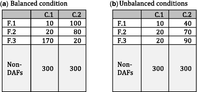
A simple example contrasting the balanced and unbalanced conditions: C.1 and C.2 are two different conditions, F.1, F.2 and F.3 are DAF, and non-DAFs are all non-DAFs across two conditions C.1and C.2

To identify DAFs consistently without being confounded by the amount of difference in total abundances of DAFs across different conditions, we propose a new approach, called Ratio Approach for Identifying Differential Abundance (RAIDA), with the assumption that majority of features are not differentially abundant. This is the same assumption used for genomic studies in DESeq (Anders and Huber, 2010) and edgeR (Robinson et al., 2010). In fact, this assumption is stronger than necessary in most cases (See the proof of Proposition in Supplementary File). RAIDA utilizes the ratios between the counts of features in each sample, eliminating possible problems associated with counts on different scales within and between conditions. Metagenomic sequencing data are sparse, i.e. containing a lot of zeros. To account for ratios with zeros, we use a modified zero-inflated lognormal (ZIL) model with the assumption that most of the zeros come from undersampling (Hughes et al., 2001) of the microbial community or insufficient sequencing depth.

We evaluated RAIDA through comprehensive simulated studies and compared the results with those of Metastats (White et al., 2009) and metagenomeSeq (Paulson et al., 2013), which were developed for a metagenomic and a microbial marker-gene analysis, respectively. In the comparison, we also included a representative method for RNA-seq analysis, edgeR, which uses TMM as a default normalization method. Compared with the other methods, RAIDA gives equivalent performance in the balanced conditions and improved performance in the unbalanced conditions. Above all, RAIDA performs consistently for both the balanced and unbalanced conditions. The consistency of the performance should be highly valued, since most of time there is no sufficient prior information about samples available. In other words, it is unlikely to know ahead that conditions to be compared are balanced or unbalanced.

We also applied RAIDA on a subset of real data selected from the original datasets in the metagenomic study of diabetes (Qin et al., 2012). RAIDA identified two differentially abundant bacteria, Clostridium botulinum and Clostridium cellulovorans, across fecal DNA samples of the type II diabetics and non-diabetic controls at the false discovery rate (FDR) < 0.05. These bacteria appear in the KEGG pathways for type II and type I diabetes mellitus, respectively. The RAIDA method is developed for the analysis of differential abundance between two conditions of samples such as healthy versus diseased. However, it can be extended to detect DAFs in metagenomic samples under more than two conditions.

2 Methods

2.1 Framework: modified ZIL model

Metagenomic sequencing data consist of highly skewed non-negative counts with an excess of zeros, which come from either true absence of microbes (true zeros) or undersampling of the microbial community (false zeros). All zeros remain unchanged after transforming the count data into ratio data using a common divisor. It can be a vector of the counts of a feature consisting of non-zeros in all samples or a vector of the sums of a group of features consisting of non-zeros in all samples. To fit ratios with zeros, we use a modified ZIL. Note a lognormal distribution has been used as a fundamental distribution for non-zero ratios in the compositional data analysis (Aitchison, 1986).

Let c_ij denote the observed count for feature i and sample j, and r_ij denote the ratio of c_ij to c_kj, where k represents a feature (or a set of features) used as a divisor and c_kj > 0 for all j. Here, $i=1,2,\dots ,n$ and $j=1,2,\dots ,m$. Throughout this article, we denote undersampling of the microbial community or insufficient sequencing depth by the false zero state. Assuming a ZIL model for the ratio R_ij, we have:

$$R_{ij}\sim \{\begin{array}{cc}0& \text{with\hspace{0.17em}\hspace{0.17em}probability\hspace{0.17em}\hspace{0.17em}}{\eta }_i\\ \text{LN}({\mu }_i,{\sigma }_i^2)& \text{\hspace{1em}with\hspace{0.17em}\hspace{0.17em}probability\hspace{0.17em}\hspace{0.17em}}1-{\eta }_i\end{array}.$$ (1)

This model does not account for zero counts from the true zeros since the support for a lognormal distribution is $(0,+\infty )$; that is, r_ij is assumed to be in the false zero state if c_ij = 0, whether or not the zero count comes from the false zero state. To accommodate for this insufficiency, a small number ϵ is added to c_ij for all i and j before computing the ratios. We denote the ratio computed this way as $R_{ij}^{\mathrm{ϵ}}$ and we have:

$$R_{ij}^{\mathrm{ϵ}}\sim \{\begin{array}{cc}\text{Unif}(0,\mathrm{ϵ})& \text{with probability }{\eta }_i\\ \text{LN}({\mu }_i,{\sigma }_i^2)& \text{\hspace{1em}with probability }1-{\eta }_i\end{array}.$$ (2)

In this study, we use $\mathrm{ϵ}=\min (r_{ij}|r_{ij}>0)$ for all i and j. The parameters ${\mathit{\theta }}_i=({\eta }_i,{\mu }_i,{\sigma }_i)$ are estimated by the following expectation-maximization (EM) algorithm.

2.2 EM algorithm

Given that a ratio R follows a lognormal distribution,

$$f_{\text{LN}}(r|\mu ,{\sigma }^2)=\frac{1}{\sigma \sqrt{2\pi }r}\exp \left[-\frac{{(\log r-\mu )}^2}{2{\sigma }^2}\right],$$ (3)

by definition $Y=\log R$ is normally distributed with mean μ and variance ${\sigma }^2$. Thus, the maximum-likelihood estimate of ${\mathit{\theta }}_i$ for the modified ZIL model, Equation (2), can be obtained by solving

(4)

where $y_{ij}=\log r_{ij}^{\mathrm{ϵ}}$, f_N is the probability density function of a normal distribution and z_ij is a unobservable latent variable that accounts for the probability of zero coming from the false zero state. The E and M steps of our EM algorithm are defined as follows:

Initialization step

Initialize the values of $({\eta }_i,{\mu }_i,{\sigma }_i)$ using ${\eta }_i^{(0)}=N_{\mathrm{ϵ}}/N$, where $N_{\mathrm{ϵ}}$ is the number of $y_{ij}\le \log \mathrm{ϵ}$ and N is the number of y_ij, ${\mu }_i^{(0)}=\text{E}(y_{ij}|y_{ij}>\log \mathrm{ϵ})$ and ${\sigma }_i^{(0)}=\text{Var}(y_{ij}|y_{ij}>\log \mathrm{ϵ})$. In cases that ${\sigma }_i^{(0)}=0$, we initialized ${\sigma }_i^{(0)}$ with ${10}^{-6}$.

E step

Estimate $Z_{ij}^{(k)}$, the probability of zero coming from the false zero state given current estimates ${\mathit{\theta }}_i^{(k)}$ by

$$Z_{ij}^{(k)}=\{\begin{array}{cc}\frac{{\eta }_i^{(k)}}{{\eta }_i^{(k)}+\left(1-{\eta }_i^{(k)}\right)\Phi \left(\sqrt{2}{\zeta }_{ij}^{(k)}\right)}& \text{\hspace{0.17em}if\hspace{0.17em}\hspace{0.17em}}{y}_{ij}\le \log \mathrm{ϵ}\\ 0& \text{\hspace{0.17em}if\hspace{0.17em}\hspace{0.17em}}{y}_{ij}>\log \mathrm{ϵ}\end{array},$$ (5)

where $\Phi$ is the cumulative distribution function of a normal distribution and ${\zeta }_{ij}^{(k)}=(y_{ij}-{\mu }_i^{(k)})/(\sqrt{2}{\sigma }_i^{(k)})$.

M step

Estimate ${\mathit{\theta }}_i^{(k+1)}$ given current estimates of $Z_{ij}^{(k)}$ by maximizing Equation (4) subject to the constraints: $0\le {\eta }_i\le 1$ and ${\sigma }_i>0$ for all i. We used a limited-memory modification of the BFGS quasi-Newton method (Byrd et al., 1995).

Repeat the E step and M step until all the parameters converge, i.e. the differences between (k + 1)th and kth estimations for all the parameters are <${10}^{-6}$.

2.3 Selection of possible common divisors

The ratio between a pair of features in samples under the same condition remains constant in the absence of random variations and the ratios between features in a sample are invariant when features are divided by a common divisor. As an illustration, consider the following example. Let $s=\{c_1,c_2,\dots ,c_n\}$ denote a sample containing counts of n features and $s\prime =\kappa ·s$ denote another sample on a different scale. Then, the ratio, for instance, between feature 1 and feature 2 in sample $s\prime$ is $(\kappa ·c_1)/(\kappa ·c_2)=c_1/c_2$, which is the same for the ratio between feature 1 and feature 2 in sample s. That is, the ratio is not affected by the scaling factor κ. Clearly the ratio between $c_1/c_n$ and $c_2/c_n$ is also $c_1/c_2$. We utilize this invariance property of ratios to identify possible common divisors across different conditions.

For each condition, we temporarily remove the features that have ≤2 non-zero counts in all samples and select a feature with non-zero counts in all the samples as a preliminary divisor. Note if no such features exist, which is very rare, we can remove some samples to have such one(s). We then obtain $r_{ij}^{\mathrm{ϵ}}$ with the preliminary divisor and estimate $\mathit{\theta }$ using the EM algorithm. The proportion of the false zero state $\mathit{\eta }$ does not carry much information in the comparison of abundances. Therefore, we simply use mean $\mathit{\mu }$ and variance ${\mathit{\sigma }}^{\mathit{2}}$ to measure the similarity in abundance between features using the Bhattacharyya distance (Aherne et al., 1998) and cluster similar features using hierarchical clustering with minimax linkage (Bien and Tibshirani, 2011) based on the Bhattacharyya distance.

2.3.1 Bhattacharyya distance

The Bhattacharyya distance has been long used as a measure of feature selection in pattern recognition, which is defined (Kailath, 1967) as

$$D_B(p,q)=-\log (BC(p,q)),$$ (6)

where p and q are probability distributions, and BC is the Bhattacharyya coefficient, which measures the amount of overlap between two distributions (Reyes-Aldasoroa and Bhalerao, 2006). For continuous probability distributions, the Bhattacharyya coefficient is defined (Kailath, 1967) as

$$BC(p,q)={\displaystyle \int \sqrt{p(x)q(x)}}dx.$$ (7)

If p and q are normal distributions, the Bhattacharyya distance has a closed form solution (Coleman and Andrews, 1979) given by

$$D_B(p,q)=\frac{1}{4}\log \left[\frac{1}{4}\left(\frac{{\sigma }_p^2}{{\sigma }_q^2}+\frac{{\sigma }_q^2}{{\sigma }_p^2}+2\right)\right]+\frac{1}{4}\left[\frac{{({\mu }_p-{\mu }_q)}^2}{{\sigma }_p^2+{\sigma }_q^2}\right].$$ (8)

2.3.2 Hierarchical clustering with minimax linkage

Hierarchical clustering builds a hierarchy of clusters commonly displayed as a tree diagram called a dendrogram, thus not requiring any pre-specified number of clusters. Instead, the hierarchy can be cut at a pre-specified level of similarity, commonly called height h, to create a set of disjoint clusters satisfying a clustering criterion. We use the clustering criterion for the minimax linkage, where for any point x the minimax linkage between two clusters C₁ and C₂ is defined as

$$d(C_1,C_2)=\underset{x\in C_1\cup C_2}{\min }\underset{x\prime \in C_1\cup C_2}{\max }d(x,x\prime ),$$ (9)

where d is a distance function (e.g. the Bhattacharyya distance). In words, the distance between C₁ and C₂ is the smallest distance to merge the two clusters and the largest distance possible between any point and the prototype that is the point giving the smallest distance among the largest distances between all paired points in C₁ and C₂. That is, for a given height h, the minimax linkage assures that the distance between any point and the prototype for a cluster is ≤h.

Cluster analysis is performed separately for each condition and we cut a minimax clustering of features with the Bhattacharyya distance at h = 0.05 that corresponds to approximately 95% overlap between two distributions. We then create a set of clustered features common in both conditions and use its elements as possible common divisors. Let’s assume, for instance, that we had a set of two clusters $\left\{\right\{A,B,E\},\{C,D\left\}\right\}$ for one condition and three clusters $\left\{\right\{A\},\{B,C,D\},\{E\left\}\right\}$ for another condition. We would then have a set of possible common divisors $\left\{\right\{A\},\{B\},\{C,D\},\{E\left\}\right\}$.

2.4 Identification of DAFs

To compare ratios across different conditions, the common divisor must be a non-DAF or a group of non-DAFs. However, the identification of non-DAFs or DAFs, which is the ultimate goal of the analysis of differential abundance, is not attainable without a priori information or assumption. Under the assumption that majority of features are not differentially abundant, the number of DAFs obtained with a non-DAF or a group of non-DAFs as a common divisor should be the smallest. This assumption is stronger than necessary in most cases as shown in the proof of Proposition (Supplementary File).

Proposition: Under the assumption that majority of features are not differentially abundant, the minimum number of DAFs is achieved when a non-DAF or a group of non-DAFs is used as a common divisor.

In other words, the common divisor that gives the smallest number of DAFs is a non-DAF or a group of non-DAFs. DAFs obtained with this common divisor are the most probable, true DAFs. To identify this common divisor and the corresponding DAFs, we repeat the following steps for each possible divisor obtained in the section 2.3:

1. Sum up the counts of features in a possible common divisor for each sample, which will reduce variation in counts across samples since the abundance of all features in a possible common divisor is assumed to be statistically identical.

2. Compute the ratios $r_{ij}^{\mathrm{ϵ}}$ with these sums as a common divisor.

3. Estimate $\mathit{\theta }$ using the EM algorithm for each condition.

4. Construct a moderated t-statistics (Smyth, 2005) for the log ratio of each feature y_ij using the estimated mean $\mathit{\mu }$ and variance ${\mathit{\sigma }}^{\mathit{2}}$ and obtain P values for the null hypotheses, $H_0:{\mu }_1={\mu }_2$ for all features.

5. Adjust P values using a multiple testing correction method. In this study, we used the Benjamini–Hochberg (BH) procedure (Benjamini and Hochberg, 1995).

6. Compute the number of DAFs.

In the step 2 earlier, if the sums contain zeros, we treat the zeros as missing values since the probability of the zeros being true zeros becomes small when a cluster contains more than a few features, that is, the zeros result most likely from undersampling. We estimate the missing values using the following steps of a parametric approach:

1. Compute the ratios of a common divisor to a feature, that has non-zero counts in all samples. Note a common divisor is in the numerator here.

2. Log-transform the non-zero ratios and estimate the mean and SD of the log-ratios.

3. Generate random normal values with the estimated mean and SD.

4. Transform log-ratios to ratios.

5. Multiply the estimated ratios by the corresponding counts of the feature.

For the temporarily removed features in the selection of possible common divisors, which have ≤2 non-zero counts in all samples in a condition, we compute their ratios using the common divisor obtained by the earlier steps after splitting them into two cases: (i) at least one non-zero in each condition and (ii) all zeros in one of conditions. We then use a two-sample moderated t-test for the first case. However, for the second case, we use a one-sample moderated t-test to test whether a distribution of ratios contains ϵ. Finally, we combine all the features and readjust P values using a multiple testing correction method, BH procedure, to control the FDR. A flow chart of RAIDA is given in Supplementary File.

3 Results

3.1 Simulation studies

To compare the performance of RAIDA to that of edgeR, metagenomeSeq and Metastats, we used simulated data where we can control the settings and the true differential abundance of each feature. We simulated counts using a zero-inflated negative binomial model:

$$C_{ij}\sim \{\begin{array}{cc}0& \text{with probability }{\xi }_i\\ \text{NB}({\mu }_i,{\gamma }_i)& \text{\hspace{1em}with probability }1-{\xi }_i\end{array},$$ (10)

where we use mean μ and size γ as the parameterization of a negative binomial, such that its probability mass function is

$$P_{NB}(C=c)=\frac{\Gamma (c+\gamma )}{\Gamma (\gamma )\Gamma (c+1)}{\left(\frac{\gamma }{\gamma +\mu }\right)}^{\gamma }{\left(\frac{\mu }{\gamma +\mu }\right)}^c,$$ (11)

giving $\text{E}(C)=\mu$ and $\text{Var}(C)=\mu +{\mu }^2/\gamma$.

To minimize any possible bias toward any method, we randomly generated the mean μ and size γ parameters from wide ranges of values partially drawn from real data (Supplementary File). For instance, the computed range of γ for non-zero counts from the real data was $(0.139,1690)$, but we used $\gamma \in (0.1,10)$ because γ is highly frequent in the range (0, 10) (Supplementary Fig. S2 in Supplementary File). It is worth noting that the analysis of differential abundance with small or moderate number of samples is often difficult when γ is small. For each condition, we sampled 1000 features with different percents—10, 20 and 30%—as DAFs, whose differences between conditions are randomly selected from 2 to 6 at varying sample sizes: m = 10, 15, 25 and 50. The sample scaling factor or the depth of coverage was also randomly selected from 1 to 10. The details for the setting of balanced and unbalanced conditions can be found in the Supplementary File. We repeated the same settings for both the balanced and unbalanced conditions. See Supplementary Table S2 in Supplementary File for further explanation and summary of parameter ranges.

We used three measures to compare the performance of the four methods: true-positive rate (TPR) versus false-positive rate (FPR), false discoveries (FD) versus features selected, and true positives and FD at a FDR of 0.05. Figure 2 shows the results of the first measure, TPR versus FPR, in terms of a partial receiver operating characteristic (ROC) analysis for four settings: 10 and 20% DAFs for the balanced and unbalanced conditions. Note that the nearer a ROC curve is to upper left corner, the better a method is. All the methods except Metastats perform similarly in the balanced conditions but not in the unbalanced conditions: there is a noticeable deterioration in performance for edgeR, metagenomeSeq and Metastats as the percent of DAFs increases. Partial ROC curve plots for different settings are given in Supplementary Figures S3, S5 and S7 in Supplementary File.

Fig. 2.

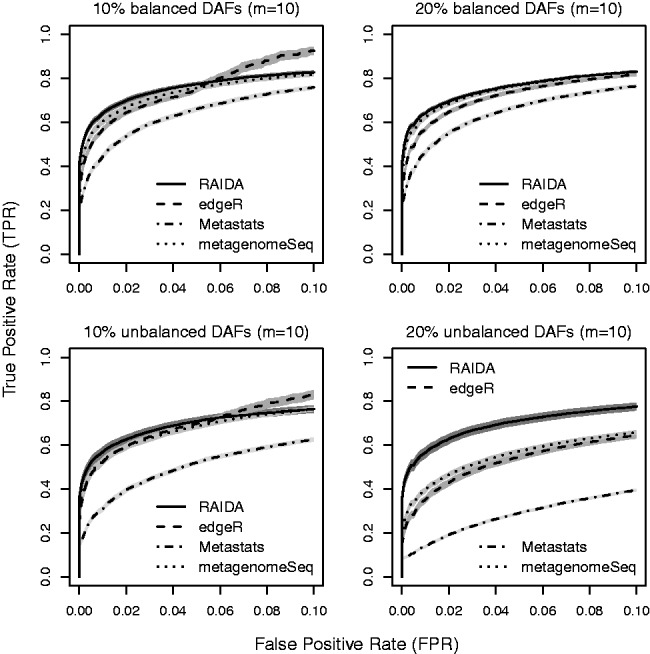
Partial of mean ROC curves for 10 and 20% of DAFs in the balanced and unbalanced conditions with 10 samples of each condition, based on 100 simulations with 1000 features. The shades around the lines are 95% confidence bands

The FD plot is often more interesting since it emphasizes the performance of a method on a selected number of significant features. Figure 3 shows FD plots for the same settings used in Figure 2. Clearly, a smaller number of FD is preferable. The performance of edgeR, metagenomeSeq and RAIDA is comparable in the balanced conditions and the 10% DAFs unbalanced conditions. However, for the 20% DAFs unbalanced conditions RAIDA results in fewer FD than the other methods. FD plots for different settings are given in Supplementary Figures S4, S6 and S8 in Supplementary File.

Fig. 3.

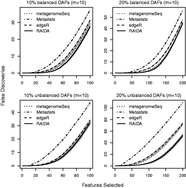
Mean false discovery plots for 10 and 20% of DAFs in the balanced and unbalanced conditions with 10 samples of each condition, based on 100 simulations with 1000 features. The horizontal axis is the number of features in ascending order of P value (i.e. the most significant feature first), and the vertical axis is the number of falsely identified features. The shades around the lines are 95% confidence bands

Figure 4 shows the numbers of true positives and false positives resulting from the four methods for the same four settings with different sample sizes: m = 10, 15, 25 and 50. Each bar represents the total number of features that statistically significant at the FDR < 0.05. The white segment in each bar is the number of true positives, and the gray segment is the number of false positives. Note the proportion of the gray segment in each bar defines the FDR. In terms of the power that is defined by the ratio of true positives to positives, metagenomeSeq and RAIDA give better results than the other two methods in all the different settings. However, metagenomeSeq has a significantly high FDR in both the balanced and unbalanced conditions. In terms of controlling FDR, edgeR performs best for the balanced conditions, and RAIDA and Metastats follow next. However, for the unbalanced conditions RAIDA surpasses edgeR as the percent of DAFs increases. As clearly shown in Figure 4, the most appealing characteristic of RAIDA is consistency in performance: the power and FDR of RAIDA depend only on the number of samples. That is, RAIDA does not depend on the amount of difference in total abundances of DAFs across different conditions, which is very critical since we do not have a priori information of metagenomic samples. The results for 30% DAFs are given in Supplementary Figure S9 in Supplementary File and it is clear that RAIDA performs comparable with other methods for the balanced conditions but exceeds others for the unbalanced situations.

Fig. 4.

Mean true and false positives plots for 10 and 20% of DAFs in the balanced and unbalanced conditions at various numbers of samples, based on 100 simulations with 1000 features. Each bar represents the total number of features that are identified as statistically significant at FDR < 0.05. The white segments are the number of true positives and the gray segments are false positives. The error bars are at a significance level of 0.05. The dotted lines indicate true numbers of DAFs. The dashed lines represent the number of DAFs designed for each situation. For example, in ‘10%’ settings there are 100 DAFs out of 1000 features

The computation time for RAIDA on a dataset containing 30 samples of 1000 features is about 30 s on a desktop with a 3.5 GHz CPU and 16 GB of memory. The comparison of computation time for the tools used in the simulation studies is given in Supplementary Table S3 in Supplementary File. The computational time for RAIDA is longer than the times for edgeR and metagenomicSeq but shorter than for Metastats.

3.2 Analysis of real data: diabetes II datasets

We applied RAIDA to 30 fecal DNA samples from male Chinese subjects with type II diabetes (N = 15) and non-diabetic controls (N = 15) (Supplementary Table S4 in Supplementary File), which were selected from 345 fecal DNA samples in the original datasets (Qin et al., 2012). We first performed sequence alignments for each sample against the bacterial reference genomes in NCBI using BLASTN and then used TAEC (Sohn et al., 2014) to estimate abundance of bacteria at the species level. The detailed information about reads and parameters used in BLASTN and TAEC is given in Supplementary File. On the count data, we applied RAIDA and identified differentially abundant species across fecal DNA samples of type II diabetics and non-diabetic controls.

The statistically significant species, at a confidence level of 95% before multiple testing correction, are shown in Figure 5. After the BH multiple testing correction, only two bacteria, C.botulinum (adjusted P value = 0.02) and C.cellulovorans (adjusted P value = 0.02), are significantly different at the FDR < 0.05. This result is similar but more specific in terms of taxonomic ranks to the previous findings (Larsen et al., 2010) obtained by real-time quantitative polymerase chain reaction and 16S rRNA gene analyses. The proportion of class Clostridia was significantly lower (P = 0.03), but the mean proportion of class Bacteroidetes was higher (not statistically significant) in the diabetics compared with the controls. Moreover, proteins produced by the bacteria C.botulinum and C.cellulovorans are involved in the KEGG pathways for type II and type I diabetes mellitus, respectively.

Fig. 5.

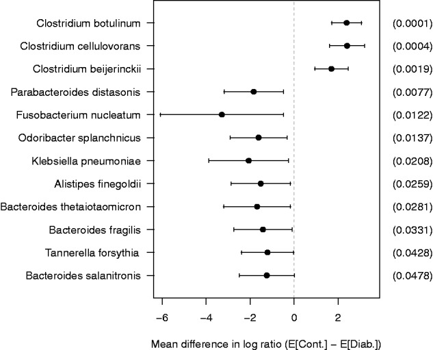
Plot of mean difference in log ratio with 95% confidence interval for the species whose P value <0.05. The mean difference is computed by subtracting the mean of diabetics from the mean of controls. The values in parentheses are raw P values

Of particular interest is the bacterium C.botulinum, which produces a highly potent neurotoxin botulinum toxin. In previous studies, botulinum toxin type A, commercially known as Botox, has been shown to improve symptoms in patients with diabetic gastroparesis (Lacy et al., 2004) and release diabetic neuropathic pain (Yuan et al., 2009). Also, Rickman and his team at the Heriot-Watt University have been observing SNARE proteins, which are known to be responsible for insulin secretion, targeted by Botox to find new methods of diagnosis and treatment for type II diabetes (http://www.hw.ac.uk/news-events/news/botoxs-target-could-hold-cure-diabetes-12960.htm). Raw and adjusted P values for the species whose raw P values are <0.05 are given in Supplementary Table S5 in Supplementary File.

4 Discussion

Even though the importance of microbial communities from the natural environment, industry and health has been well acknowledged, the composition of microbial communities is still barely known. Therefore, a method for identifying DAFs in metagenomic samples should not depend on characteristics of microbial communities across different conditions, such as the amount of difference in total abundances of DAFs across different conditions. RAIDA has been developed to satisfy this essential criterion, specifically for the analysis of differential abundance across different, but closely related conditions, such as healthy and diseased, where majority of features are unlikely differentially abundant across conditions. We have shown the consistency of RAIDA on various types of samples in the simulation study.

In this study, we used the smallest non-zero ratio for the value of ϵ in our modified ZIL model, Equation (2). However, some other quantities such as the smallest number in the 5th percentile can be used in the estimation of DAFs across different conditions. As an illustration, we analyzed the simulated data for the 10 and 20% DAFs in the balanced and unbalanced conditions for the sample size m = 15 using the smallest number in the 5th percentile for ϵ. We then compared results with those obtained using the smallest non-zero ratio for ϵ. Both the values of ϵ give almost identical results in terms of TPR and FPR as shown in Supplementary Figure S10 in Supplementary File.

A non-DAF can be a common divisor but will not provide reliable results if the non-DAF contains more than a few zeros, which is often the case, because all the zeros will be treated as missing values and estimated even if some zeros are truly zero. It will be similar for a group of non-DAFs with a few members. Since we assume that the majority of features are not differentially abundant, it is highly probable that non-DAFs form one of the largest cluster. Therefore, it is more practical to use only the clusters with larger numbers of features as possible common divisors.

We have optimized our calculations to the analysis of differential abundance between two conditions of samples such as healthy versus diseased in this article. However, our method can be easily extended to more than two conditions. Note it is just a two-sample t-test with modified variances for two conditions. Thus, for more than two conditions, the test will be just the analysis of variance with modified variances. Nevertheless, our method may not be applicable for too many conditions where a common divisor with more than one feature for all conditions may not exist. Moreover, even though we have developed our method for metagenomic data, our method should be applicable to other types of count data such as RNA-seq data. However, our method might not be appropriate for the comparison of environmentally different samples (e.g. soil versus sea water, or human gut versus soil), where the assumption that majority of features are not differentially abundant could be violated.

Funding

This work was supported by National Science Foundation [DMS-1043080 and DMS-1222592 to L.A] and partially supported by National Institutes of Health [P30 ES006694 to L.A] and United States Department of Agriculture [Hatch project, ARZT-1360830-H22-138 to L.A].

Conflict of Interest: none declared.

References

- Aherne F.J., et al. (1998) The Bhattacharyya metric as an absolute similarity measure for frequency coded data. Kybernetika, 34, 363–368. [Google Scholar]
- Aitchison J. (1986) The Statistical Analysis of Compositional Data. 1st edn Chapman and Hall, New York. [Google Scholar]
- Anders S., Huber W. (2010) Differential expression analysis for sequence count data. Genome Biol., 11, R106. [DOI] [PMC free article] [PubMed] [Google Scholar]
- Benjamini Y., Hochberg Y. (1995) Controlling the false discovery rate: a practical and powerful approach to multiple testing. J. R. Stat. Soc. B. 57, 289–300. [Google Scholar]
- Bien J., Tibshirani R. (2011) Hierarchical clustering with prototypes via minimax linkage. J. Am. Stat. Assoc., 106, 1075–1084. [DOI] [PMC free article] [PubMed] [Google Scholar]
- Byrd R.H., et al. (1995) A limited memory algorithm for bound constrained optimization. SIAM J. Sci. Comput., 16, 1190–1208. [Google Scholar]
- Coleman G.B., Andrews H.C. (1979) Image segmentation by clustering. Proc IEEE, 67, 773–785. [Google Scholar]
- Dillies M.A., et al. (2013) A comprehensive evaluation of normalization methods for Illumina high-throughput RNA sequencing data analysis. Brief. Bioinform., 14, 671–83. [DOI] [PubMed] [Google Scholar]
- Hughes J.B., et al. (2001) Counting the uncountable: statistical approaches to estimating microbial diversity. Appl. Environ. Microbiol., 67, 4399–4406. [DOI] [PMC free article] [PubMed] [Google Scholar]
- Kailath T. (1967) The divergence and Bhattacharyya distance measures in signal selection. IEEE Trans. Commun., 15, 52–60. [Google Scholar]
- Lacy B.E., et al. (2004) The treatment of diabetic gastroparesis with botulinum toxin injection of the pylorus. Diabetes Care, 27, 2341–2347. [DOI] [PubMed] [Google Scholar]
- Larsen N., et al. (2010) Gut microbiota in human adults with type 2 diabetes differs from non-diabetic adults. PLoS One, 5, e9085. [DOI] [PMC free article] [PubMed] [Google Scholar]
- Paulson J.N., et al. (2013) Differential abundance analysis for microbial marker–gene surveys. Nat. Methods, 10, 1200–1202. [DOI] [PMC free article] [PubMed] [Google Scholar]
- Qin J., et al. (2012) A metagenome-wide association study of gut microbiota in type 2 diabetes. Nature, 490, 55–60. [DOI] [PubMed] [Google Scholar]
- Reyes-Aldasoroa C.C., Bhalerao A. (2006) The Bhattacharyya space for feature selection and its application to texture segmentation. Pattern Recognit., 39, 812–826. [Google Scholar]
- Robinson M.D., Oshlack A. (2010) A scaling normalization method for differential expression analysis of RNA-seq data. Genome Biol., 11, R25. [DOI] [PMC free article] [PubMed] [Google Scholar]
- Robinson M.D., et al. (2010) edgeR: a Bioconductor package for differential expression analysis of digital gene expression data. Bioinformatics, 26, 139–140. [DOI] [PMC free article] [PubMed] [Google Scholar]
- Schloss P.D., Handelsman J. (2005) Metagenomics for studying unculturable microorganisms: cutting the Gordian knot. Genome Biol., 6, 229. [DOI] [PMC free article] [PubMed] [Google Scholar]
- Smyth G.K. (2005) Limma: linear models for microarray data. In: Gentleman R., et al. (eds.) Bioinformatics and Computational Biology Solutions using R and Bioconductor. Springer, New York, pp. 397–420. [Google Scholar]
- Sohn M.B., et al. (2014) Accurate genome relative abundance estimation for closely related species in a metagenomic sample. BMC Bioinformatics, 15, 242. [DOI] [PMC free article] [PubMed] [Google Scholar]
- Thomas T., et al. (2012) Metagenomics - a guide from sampling to data analysis. Microb. Inform. Exp., 2, 3. [DOI] [PMC free article] [PubMed] [Google Scholar]
- Virgin H.W., Todd J.A. (2011) Metagenomics and Personalized Medicine. Cell, 147, 44–56. [DOI] [PMC free article] [PubMed] [Google Scholar]
- White J.R., et al. (2009) Statistical methods for detecting differentially abundant features in clinical metagenomic samples. PLoS Comput. Biol., 5, e1000352. [DOI] [PMC free article] [PubMed] [Google Scholar]
- Yuan R.Y., et al. (2009) Botulinum toxin for diabetic neuropathic pain: A randomized double-blind crossover trial. Neurology, 72, 1473–1478. [DOI] [PubMed] [Google Scholar]
Associated Data
This section collects any data citations, data availability statements, or supplementary materials included in this article.